Point-Voxel Adaptive Feature Abstraction for Robust Point Cloud Classification

Lifa Zhu Affiliation: DeepGlint, Beijing, China Changwei Lin Affiliation: DeepGlint, Beijing, China Chen Zheng Affiliation: China University of Mining and Technology, Beijing, China E-mail zhulf0804@gmail.com Ninghua Yang E-mail {changweilin,ninghuayang}@deepglint.com E-mail zc824435664@163.com Affiliation: DeepGlint, Beijing, China

Abstract

Great progress has been made in point cloud classification with learning-based methods. However, complex scene and sensor inaccuracy in real-world application make point cloud data suffer from corruptions, such as occlusion, noise and outliers. In this work, we propose Point-Voxel based Adaptive (PV-Ada) feature abstraction for robust point cloud classification under various corruptions. Specifically, the proposed framework iteratively voxelize the point cloud and extract point-voxel feature with shared local encoding and Transformer. Then, adaptive max-pooling is proposed to robustly aggregate the point cloud feature for classification. Experiments on ModelNet-C dataset demonstrate that PV-Ada outperforms the state-of-the-art methods. In particular, we rank the $2^{nd}$ place in ModelNet-C classification track of PointCloud-C Challenge 2022, with Overall Accuracy (OA) being 0.865. Code will be available at https://github.com/zhulf0804/PV-Ada.

Keywords:

point-voxel, adaptive feature abstraction, robust classification

1 Introduction

Point cloud classification, as one of the important 3D tasks, has achieved remarkable progress[15, 16, 22, 8, 23, 3, 28, 11, 12]. However, the state-of-the-art methods are less robust in 3D point cloud recognition under corruptions or attack[17, 21, 20, 14]. In this report, we mainly describe our method and experiments on ModelNet-C point cloud classification hosted in PointCloud-C Challenge 2022¹¹ 1 https://pointcloud-c.github.io/competition.html, which benchmarks point cloud robustness analysis under corruptions[17].

ModelNet-C is the first systematically-designed test-suite for point cloud classification under corruptions[17]. It extends the validation set of ModelNet40 with the proposed atomic corruptions, including “Add Global”, “Add Local”, “Drop Global”, “Drop Local”, “Rotate”, “Scale” and “Jitter”. Moreover, each atomic corruption is performed with 5 severity levels. It’s noted that each real-world corruption can be broken down into a combination of the atomic corruptions.

In terms of the corruptions in ModelNet-C data, we propose Point-Voxel Adaptive (PV-Ada) feature abstraction for robust point cloud classification. PV-Ada is proposed based on the following two observations. First, the rough contour may benefit point cloud classification under corruptions, instead of paying attention to detailed structures. It inspires us to involve both voxel-level and point-level feature for point cloud classification. Second, not all all points in point cloud are equal for individual feature representation, such as plane points and outlier points. So we propose to learn point weight in an end-to-end manner, thus conducting adaptive pooling for robust feature abstraction.

Experiments on ModelNet-C and ModelNet demonstrate the effectiveness of PV-Ada. Our method outperforms the state-of-the-art published models and achieves 0.884 and 0.865 OA on the public and private ModelNet-C test set, respectively.

2 Method

A point cloud is represented as a set $\mathcal{X}=\{\mathbf{x}_{i}\in\mathbb{R}^{3}\}_{i=1,2,\cdots,N}$ , where $N$ is the point number in $\mathcal{X}$ . For the convenience of following discussion, point cloud is denoted by matrix $\mathbf{X}\in\mathbb{R}^{N\times 3}$ . Inputted point cloud $\mathbf{X}$ , PV-Ada outputs $C$ scores for all the $C$ candidate categories. The overall architecture of PV-Ada is depicted in Fig. 1.

2.1 Point-voxel encoder

Point-voxel as input and voxelization operation have been widely used in point cloud detection, segmentation and classification[18, 19, 10, 24, 7, 9, 22, 2, 1], which shows the effectiveness and efficiency of voxelization. Our presented point-voxel encoder consists of three modules: local encoding, Transformer and pyramid feature interaction.

Local encoding

Local encoding groups $k$ nearest neighbors for each point (voxel), then learns $D$ dimensional point (voxel) feature through convolution and non-linear operations. Take $\mathbf{X}\in\mathbb{R}^{N\times 3}$ as an example, local encoding outputs its local desciptor $\mathbf{F}_{\mathbf{X}}^{e}\in\mathbb{R}^{N\times D}$ .

Transformer

We adopt PCT[3] to enhance the point feature for point cloud. Take $\mathbf{X}$ as an example, it first further encode point feature $\mathbf{F}_{\mathbf{X}}^{e}$ with MLP and non-linear operations, generating $D$ dimensional features $\mathbf{F}_{\mathbf{X}}^{m}\in\mathbb{R}^{N\times D}$ . Then four offset-attention are introduced to obtain features $(\mathbf{F}_{\mathbf{X}}^{oa_{1}},\mathbf{F}_{\mathbf{X}}^{oa_{2}},\mathbf{F}_{\mathbf{X}}^{oa_{3}},\mathbf{F}_{\mathbf{X}}^{oa_{4}})\in\mathbb{R}^{N\times D}$ . Each is generated through a vanilla attention and a offset-based residual structure:

$\displaystyle\mathbf{F}_{\mathbf{X}}^{oa_{0}}$	$\displaystyle=\mathbf{F}_{\mathbf{X}}^{m},$	(1)
$\displaystyle\mathbf{F}_{\mathbf{X}}^{va_{i}}$	$\displaystyle=\text{VanillaAttention}(\mathbf{F}_{\mathbf{X}}^{oa_{i-1}}),\quad i=1,2,3,4,$
$\displaystyle\mathbf{F}_{\mathbf{X}}^{oa_{i}}$	$\displaystyle=\mathbf{F}_{\mathbf{X}}^{oa_{i-1}}+f_{i}(\mathbf{F}_{\mathbf{X}}^{oa_{i-1}}-\mathbf{F}_{\mathbf{X}}^{va_{i}}),$

where $f_{i}(\cdot)$ is implemented using Conv1d, normalization and ReLU.

Finally, the feature $\mathbf{F}_{\mathbf{X}}^{t}\in\mathbb{R}^{N\times{4D}}$ outputted from Transformer is calculated through:

\displaystyle\mathbf{F}_{\mathbf{X}}^{t}

\displaystyle=f_{5}(\text{cat}([\mathbf{F}_{\mathbf{X}}^{e},\mathbf{F}_{\mathbf{X}}^{oa_{1}},\mathbf{F}_{\mathbf{X}}^{oa_{2}},\mathbf{F}_{\mathbf{X}}^{oa_{3}},\mathbf{F}_{\mathbf{X}}^{oa_{4}}])),

(2)

where $\text{cat}(\cdot)$ is concatenation, $f_{5}(\cdot)$ is implemented using Conv1d, normalization and LeakyReLU.

Refer to caption — Figure 1: The overall architecture of PV-Ada for point cloud classification. It takes original point cloud $\mathbf{X}$ as input and outputs $C$ confidence scores $\mathbf{Y}$ . The modules of pyramid feature interaction and adaptive feature abstraction are detailed in Section 2.1 and Section 2.2 respectively.

Pyramid feature interaction

As presented in Fig. 1, we progressively voxelize the input point cloud $\mathbf{X}$ twice with voxel size $v$ and $2v$ , denoting the voxelized point clouds as $\mathbf{X^{\prime}}\in\mathbb{R}^{N^{\prime}\times 3}$ and $\mathbf{X^{\prime\prime}}\in\mathbb{R}^{N^{\prime\prime}\times 3}$ . Pyramid feature interaction is conducted in two aspects. For one hand, local encoding and Transformer are weight-shared across $\mathbf{X}$ , $\mathbf{X^{\prime}}\in\mathbb{R}^{N^{\prime}\times 3}$ and $\mathbf{X^{\prime\prime}}\in\mathbb{R}^{N^{\prime\prime}\times 3}$ . For the other hand, we devised feature interaction operator $z(\cdot,\cdot)$ to reuse learned fine-grained features. Three functions are considered:

$\displaystyle z_{1}(\mathbf{F}^{1},\mathbf{F}^{2})$	$\displaystyle=\mathbf{F}^{2},$	(3)
$\displaystyle z_{2}(\mathbf{F}^{1},\mathbf{F}^{2})$	$\displaystyle=h_{1}(\mathbf{F}^{1})+\mathbf{F}^{2},$
$\displaystyle z_{3}(\mathbf{F}^{1},\mathbf{F}^{2})$	$\displaystyle=h_{3}(\text{cat}([h_{2}(\mathbf{F}^{1}),\mathbf{F}^{2}])),$

where $h_{1}(\cdot),h_{2}(\cdot)$ and $h_{3}(\cdot)$ are composed of Conv1d, normalization and LeakyReLU operations used for modifying feature dimensions. Finally, $\mathbf{F}_{\mathbf{X}^{\prime}}^{t}\in\mathbb{R}^{N^{\prime}\times{4D}},\mathbf{F}_{\mathbf{X}^{\prime\prime}}^{t}\in\mathbb{R}^{N^{\prime\prime}\times{4D}}$ are obtained in the same way as $\mathbf{F}_{\mathbf{X}}^{t}$ . All of them are utilized in the following adaptive feature abstraction.

2.2 Adaptive feature abstraction

Inspired by IA-SSD[27] and NgeNet[29], we noticed that the idea of not all points being equal/important also applies to point cloud classification.

Adaptive feature abstraction takes $\mathbf{F}_{\mathbf{X}}^{t}\in\mathbb{R}^{N\times{4D}}$ as input and outputs point score $\mathbf{S}_{\mathbf{X}}^{t}\in\mathbb{R}^{N\times{1}}$ for the following pooling operation:

	$\displaystyle\mathbf{S}_{\mathbf{X}}^{t}$	$\displaystyle=g(\mathbf{F}_{\mathbf{X}}^{t}),$		(4)
	$\displaystyle\mathbf{F}_{\mathbf{X}}$	$\displaystyle=\text{MaxPooling}(\mathbf{S}_{\mathbf{X}}^{t}\cdot\mathbf{F}_{\mathbf{X}}^{t}),$		(4)

where $g(\cdot)$ is implemented by Conv1d and $\mathbf{F}_{\mathbf{X}}\in\mathbb{R}^{4D}$ . $\mathbf{F}_{\mathbf{X}^{\prime}}\in\mathbb{R}^{4D}$ and $\mathbf{F}_{\mathbf{X}^{\prime\prime}}\in\mathbb{R}^{4D}$ are obtained in the same way, but learned parameters are not shared in the respective $g(\cdot)$ .

We concat $\mathbf{F}_{\mathbf{X}}$ , $\mathbf{F}_{\mathbf{X}^{\prime}}$ and $\mathbf{F}_{\mathbf{X}^{\prime\prime}}$ as input, $C$ dimension score vector $\mathbf{Y}$ is outputted through MLPs.

2.3 Loss

Cross entropy loss with label smoothing is adopted in our model. Given predicted score $\mathbf{Y}\in\mathbb{R}^{C}$ and the ground truth one-hot label $\hat{\mathbf{Y}}\in\{0,1\}^{C}$ , loss function is defined as

	$\displaystyle\hat{\mathbf{y}}^{soft}_{i}$	$\displaystyle=\hat{\mathbf{y}}_{i}\cdot(1-\alpha)+(1-\hat{\mathbf{y}}_{i})\cdot\alpha/(C-1),$		(5)
	$\displaystyle\mathcal{L}$	$\displaystyle=-\sum_{i=0}^{C-1}{\hat{\mathbf{y}}^{soft}_{i}\cdot\log\text{softmax}(\mathbf{y}_{i})},$		(5)

where $\alpha$ is a label smoothing parameter.

3 Experiments

3.1 Datasets

Training set

We use ModelNet40[25] training set for model training. It collects 9,843 (of total 12, 311) CAD models from 40 man-made categories. In consistent with PointNet[15], 1024 points are sampled from each aligned CAD model and then are normalized into a unit sphere.

Validation set

The proposed public ModelNet-C[17] is as our validation set, which corrupts ModelNet40 test set with the aforementioned 7 atomic corruptions at 5 severity levels. In total, 35 corrupted sets are generated, with each contains 2468 point clouds. It’s noted that points in different set may be different. For example, there are 524 and 1524 points in ”Drop Local” set and ”“Add Local” set at severity level 5, respectively.

Testing set

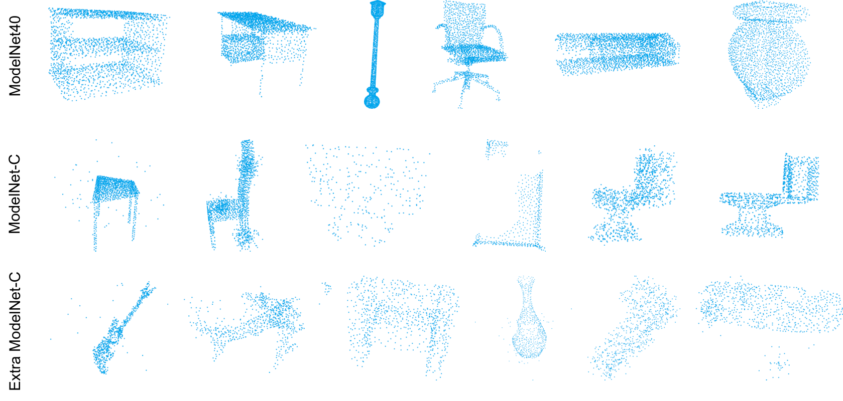
Test set is generated by a combination of different corruptions, rather than the separated ones in ModelNet-C, which is much more challenging. There are 24680 point clouds in total, and each contains 724 points. Some examples of training set, validation set and testing set are visualized in Fig. 2.

3.2 Evaluation metric

Overall Accuracy (OA) or Corruption Error (CE) [4] are adopted to evaluate model performance on validation set and testing set. CE and mCE are calculated[17]:

	$\displaystyle\text{CE}_{i}$	$\displaystyle=\frac{\sum_{l=1}^{5}(1-\text{OA}_{i,l})}{\sum_{l=1}^{5}(1-\text{OA}_{i,l}^{\text{DGCNN}})},$		(6)
	$\displaystyle\text{mCE}$	$\displaystyle=\frac{1}{N}\sum_{i=1}^{N}\text{CE}_{i},$		(6)

where $\text{OA}_{i,l}$ is the overall accuracy on corrupted set using corruption type $i$ at severity level $l$ , $\text{OA}_{i,l}^{\text{DGCNN}}$ is the baseline overall accuracy using DGCNN[23], and $N=7$ is the number of atomic corruption types.

3.3 Implementation details

PV-Ada is implemented with PyTorch[13]. We train the model 350 epochs on a single RTX3090 GPU card with batch size 64. SGD is used with initial learning rate 0.1, momentum 0.9 and weight decay 0.0005. Learning rate is scheduled using a cosine annealing with $T_{\max}=350$ and $\eta_{\min}=0.001$ . Voxel size $v$ is set to 0.05, $k$ in local encoding is set to 32, feature dimension $D$ is set to 128, and label smoothing parameter $\alpha$ is set to 0.2.

Data augmentation

In consistent with [17], three augmentations are utilized in our model: random anisotropic scaling in the range $[\frac{2}{3},\frac{3}{2}]$ , random translation in the range $[-0.2,0.2]$ and WOLFMix. WOLFMix is designed based on PointWOLF[5] and RSMix[6]. Different from RPC[17], which leverages RSMix augmentation in probability in each iteration, we always leverage RSMix augmentation for the final 50 epochs during training. Besides, we explore other data augmentation, such as Tapering[14], in our experiments.

3.4 Comparison to the state-of-the-arts

Results for overall accuracy on testing set (ExtraOA), validation set (mOA) and clean ModelNet40 testing set are reported in Table 1. Equipped with WOLFMix, we achieve 0.860 ExtraOA, improving 6.3% compared with the state-of-the-art methods. We achieve 0.884 mOA on the validation set, outperforming all the published methods. Detailed results on the 7 corruption sets are also reported. We improve accuracy on ”Jitter” set compared to PCT, GDANet and RPC, while the performance on other corruption sets does not deteriorate significantly. We achieve 0.923 on the clean ModelNet-40 testing set. Though droping about 1% compared to the SOTA models, a relative lower baseline is adopted as our model(see Table 3). With Tapering augmentation, we achieve 0.865 ExtraOA on the testing set. Results for mCE are reported in Table 2, where we achieve the lowest mCE on validation set.

Table 1: Full results for Overall Accuracy (OA) on testing set (ExtraOA), validation set (mOA) and clean ModelNet40 testing set. W.M. is short for WOLFMix and Tp is short for Tapering. Bold: best in column. Underline: second best in column.

	ExtraOA $\uparrow$	Clean $\uparrow$	mOA $\uparrow$	Scale	Jitter	Drop-G	Drop-L	Add-G	Add-L	Rotate
PointNet[15]+W.M.	-	0.884	0.743	0.801	0.850	0.857	0.776	0.343	0.807	0.768
PCT[3]+W.M.	-	0.934	0.873	0.906	0.730	0.906	0.898	0.912	0.861	0.895
GDANet[26]+W.M.	0.797	0.934	0.871	0.915	0.721	0.868	0.886	0.910	0.886	0.912
RPC[17]+W.M.	0.739	0.933	0.865	0.905	0.694	0.895	0.894	0.902	0.868	0.897
PV-Ada+W.M.	0.860	0.923	0.884	0.911	0.796	0.9	0.88	0.915	0.89	0.896
PV-Ada+W.M.+Tp	0.865	0.911	0.88	0.907	0.792	0.897	0.874	0.914	0.884	0.892

Table 2: Full results for mCE on validation set. Bold: best in column. Underline: second best in column.

	mCE $\downarrow$	Scale	Jitter	Drop-G	Drop-L	Add-G	Add-L	Rotate
DGCNN[23]+W.M.	0.590	0.989	0.715	0.698	0.575	0.285	0.415	0.451
PCT[3]+W.M.	0.574	1.000	0.854	0.379	0.493	0.298	0.505	0.488
GDANet[26]+W.M.	0.571	0.904	0.883	0.532	0.551	0.305	0.415	0.409
RPC[17]+W.M.	0.601	1.011	0.968	0.423	0.512	0.332	0.480	0.479
PV-Ada+W.M.	0.538	0.947	0.652	0.403	0.58	0.292	0.4	0.493

3.5 Ablation studies

Ablation studies on the proposed modules are summarized in Table 3.

Base

One classification model whose backbone is composed of simple local encoding and Transformer is adopted as the baseline model.

P-V

With Point-Voxel architecture whose local encoding and Transformer shared, the accuracy on validation set is improved by 1.7%.

Best val

We choose the weight with best performance on validation set, instead of on clean ModelNet40 testing set. With this trick, we achieve 0.848 ExtraOA, improving 0.5% on testing set.

RSMix

RSMix is always leveraged in the final 50 epochs during training. With this trick, we achieved 0.855 ExtraOA on testing set.

AFA

Adaptive feature abstraction is the proposed module introduced in 2.2. With AFA module, we achieve 0.860 ExtraOA on testing set.

Tapering

With Tapering augmentation, we achieve the best ExtraOA 0.865 on testing set. However, performance on both validation set and clean ModelNet40 ‘testing set‘ drops. Also, we observed that training with Tapering is not stable. We didn’t conduct more experiments on Tapering.

Except the above proposed modules and positive tricks, we also explore other module designs. The results are summarized in Table 4.

Table 3: Ablation studies on the proposed modules and positive tricks on ModelNet-C.

Base	P-V	Best val	RSMix	AFA	Tapering	clean $\uparrow$	mOA $\uparrow$	ExtraOA $\uparrow$
✓						0.928	0.862	-
✓	✓					0.927	0.879	0.843
✓	✓	✓				0.923	0.881	0.848
✓	✓	✓	✓			0.921	0.882	0.855
✓	✓	✓	✓	✓		0.923	0.884	0.860
✓	✓	✓	✓	✓	✓	0.911	0.88	0.865

Table 4: Ablation studies on the negative designed modules.

Model	clean $\uparrow$	mOA $\uparrow$
Base + P-V ( $z_{1}$ )	0.927	0.879
Base + P-V ( $z_{2}$ )	0.932	0.862
Base + P-V ( $z_{3}$ )	0.926	0.868
Base + P-V (share)	0.927	0.879
Base + P-V (w.o. share)	0.929	0.855
Base + P-V (#2 voxel)	0.927	0.879
Base + P-V (#3 voxel)	0.914	0.868

Pyramid feature interaction

We compare the performance between $z_{1}(\cdot,\cdot)$ , $z_{2}(\cdot,\cdot)$ and $z_{3}(\cdot,\cdot)$ . As shown the top-3 lines in Table 4, the highest mOA 0.879 is achieved with $z_{1}(\cdot,\cdot)$ . It indicates that better performance may be obtained if there is no feature interaction.

Shared weights

Higher mOA is obtained when the weights are shared by local encoding and Transformer modules. Meanwhile, less parameters are needed when the weights are shared in some modules.

The times of iterative voxelization

We increase the iterative voxlization times to 3 and achieve the worse mOA 0.868. The reason for this maybe the voxel size ( $4v$ ) is too large for ModelNet and ModelNet-C.

3.6 Model size and inference time

The model size and inference time are reported in Table 5. There are about 3.16M parameters in PV-Ada. Inference time is averaged on testing set using batch size 1 to predict.

Table 5: Model size and inference time

Model	# parameters	inference time
PV-Ada	3.16 M	15.7 ms

4 Discussion and conclusion

Equipped with a stronger backbone, better performance may be achieved in point cloud classification under corruptions. Data augmentations, such as Tapering, Twisting and Shearing are not fully explored in our experiments, and we are not sure whether they are positive for model training.

In this report, we propose PV-Ada for robust point cloud classification under corruptions. Point-voxel encoder with shared local encoding and Transformer is introduced for point feature extraction. Then adaptive feature abstraction is proposed for point cloud representation. With several tricks, our PV-Ada ranks the second place in ModelNet-C classification track of PointCloud-C Challenge 2022, with ExtraOA being 0.865. Additional, PV-Ada outperforms the published state-of-the-art motheds on ModelNet-C dataset.

References

[1] Choy, C., Gwak, J., Savarese, S.: 4d spatio-temporal convnets: Minkowski convolutional neural networks. In: Proceedings of the IEEE Conference on Computer Vision and Pattern Recognition. pp. 3075–3084 (2019)
[2] Choy, C., Park, J., Koltun, V.: Fully convolutional geometric features. In: Proceedings of the IEEE/CVF International Conference on Computer Vision. pp. 8958–8966 (2019)
[3] Guo, M.H., Cai, J.X., Liu, Z.N., Mu, T.J., Martin, R.R., Hu, S.M.: Pct: Point cloud transformer. Computational Visual Media 7(2), 187–199 (2021)
[4] Hendrycks, D., Dietterich, T.: Benchmarking neural network robustness to common corruptions and perturbations. arXiv preprint arXiv:1903.12261 (2019)
[5] Kim, S., Lee, S., Hwang, D., Lee, J., Hwang, S.J., Kim, H.J.: Point cloud augmentation with weighted local transformations. In: Proceedings of the IEEE/CVF International Conference on Computer Vision. pp. 548–557 (2021)
[6] Lee, D., Lee, J., Lee, J., Lee, H., Lee, M., Woo, S., Lee, S.: Regularization strategy for point cloud via rigidly mixed sample. In: Proceedings of the IEEE/CVF Conference on Computer Vision and Pattern Recognition. pp. 15900–15909 (2021)
[7] Li, J., Dai, H., Shao, L., Ding, Y.: From voxel to point: Iou-guided 3d object detection for point cloud with voxel-to-point decoder. In: Proceedings of the 29th ACM International Conference on Multimedia. pp. 4622–4631 (2021)
[8] Li, Y., Bu, R., Sun, M., Wu, W., Di, X., Chen, B.: Pointcnn: Convolution on x-transformed points. Advances in neural information processing systems 31 (2018)
[9] Liu, Z., Tang, H., Lin, Y., Han, S.: Point-voxel cnn for efficient 3d deep learning. Advances in Neural Information Processing Systems 32 (2019)
[10] Liu, Z., Tang, H., Zhao, S., Shao, K., Han, S.: Pvnas: 3d neural architecture search with point-voxel convolution. arXiv preprint arXiv:2204.11797 (2022)
[11] Ma, X., Qin, C., You, H., Ran, H., Fu, Y.: Rethinking network design and local geometry in point cloud: A simple residual mlp framework. arXiv preprint arXiv:2202.07123 (2022)
[12] Pang, Y., Wang, W., Tay, F.E., Liu, W., Tian, Y., Yuan, L.: Masked autoencoders for point cloud self-supervised learning. arXiv preprint arXiv:2203.06604 (2022)
[13] Paszke, A., Gross, S., Massa, F., Lerer, A., Bradbury, J., Chanan, G., Killeen, T., Lin, Z., Gimelshein, N., Antiga, L., et al.: Pytorch: An imperative style, high-performance deep learning library. Advances in neural information processing systems 32 (2019)
[14] Pérez, J.C., Alfarra, M., Giancola, S., Ghanem, B., et al.: 3deformrs: Certifying spatial deformations on point clouds. In: Proceedings of the IEEE/CVF Conference on Computer Vision and Pattern Recognition. pp. 15169–15179 (2022)
[15] Qi, C.R., Su, H., Mo, K., Guibas, L.J.: Pointnet: Deep learning on point sets for 3d classification and segmentation. In: Proceedings of the IEEE conference on computer vision and pattern recognition. pp. 652–660 (2017)
[16] Qi, C.R., Yi, L., Su, H., Guibas, L.J.: Pointnet++: Deep hierarchical feature learning on point sets in a metric space. Advances in neural information processing systems 30 (2017)
[17] Ren, J., Pan, L., Liu, Z.: Benchmarking and analyzing point cloud classification under corruptions. International Conference on Machine Learning (ICML) (2022)
[18] Shi, S., Guo, C., Jiang, L., Wang, Z., Shi, J., Wang, X., Li, H.: Pv-rcnn: Point-voxel feature set abstraction for 3d object detection. In: Proceedings of the IEEE/CVF Conference on Computer Vision and Pattern Recognition. pp. 10529–10538 (2020)
[19] Shi, S., Jiang, L., Deng, J., Wang, Z., Guo, C., Shi, J., Wang, X., Li, H.: Pv-rcnn++: Point-voxel feature set abstraction with local vector representation for 3d object detection. arXiv preprint arXiv:2102.00463 (2021)
[20] Sun, J., Nie, W., Yu, Z., Mao, Z.M., Xiao, C.: Pointdp: Diffusion-driven purification against adversarial attacks on 3d point cloud recognition. arXiv preprint arXiv:2208.09801 (2022)
[21] Sun, J., Zhang, Q., Kailkhura, B., Yu, Z., Xiao, C., Mao, Z.M.: Benchmarking robustness of 3d point cloud recognition against common corruptions. arXiv preprint arXiv:2201.12296 (2022)
[22] Thomas, H., Qi, C.R., Deschaud, J.E., Marcotegui, B., Goulette, F., Guibas, L.J.: Kpconv: Flexible and deformable convolution for point clouds. In: Proceedings of the IEEE/CVF international conference on computer vision. pp. 6411–6420 (2019)
[23] Wang, Y., Sun, Y., Liu, Z., Sarma, S.E., Bronstein, M.M., Solomon, J.M.: Dynamic graph cnn for learning on point clouds. Acm Transactions On Graphics (tog) 38(5), 1–12 (2019)
[24] Wu, P., Gu, L., Yan, X., Xie, H., Wang, F.L., Cheng, G., Wei, M.: Pv-rcnn++: Semantical point-voxel feature interaction for 3d object detection. arXiv preprint arXiv:2208.13414 (2022)
[25] Wu, Z., Song, S., Khosla, A., Yu, F., Zhang, L., Tang, X., Xiao, J.: 3d shapenets: A deep representation for volumetric shapes. In: Proceedings of the IEEE conference on computer vision and pattern recognition. pp. 1912–1920 (2015)
[26] Xu, M., Zhang, J., Zhou, Z., Xu, M., Qi, X., Qiao, Y.: Learning geometry-disentangled representation for complementary understanding of 3d object point cloud. In: Proceedings of the AAAI Conference on Artificial Intelligence. vol. 35, pp. 3056–3064 (2021)
[27] Zhang, Y., Hu, Q., Xu, G., Ma, Y., Wan, J., Guo, Y.: Not all points are equal: Learning highly efficient point-based detectors for 3d lidar point clouds. In: Proceedings of the IEEE/CVF Conference on Computer Vision and Pattern Recognition. pp. 18953–18962 (2022)
[28] Zhao, H., Jiang, L., Jia, J., Torr, P.H., Koltun, V.: Point transformer. In: Proceedings of the IEEE/CVF International Conference on Computer Vision. pp. 16259–16268 (2021)
[29] Zhu, L., Guan, H., Lin, C., Han, R.: Neighborhood-aware geometric encoding network for point cloud registration. arXiv preprint arXiv:2201.12094 (2022)