Implications of sparsity and high triangle density for graph representation learning
Hannah Sansford Alexander Modell Nick Whiteley Patrick Rubin-Delanchy
University of Bristol University of Bristol University of Bristol University of Bristol
Abstract
Recent work has shown that sparse graphs containing many triangles cannot be reproduced using a finite-dimensional representation of the nodes, in which link probabilities are inner products. Here, we show that such graphs can be reproduced using an infinite-dimensional inner product model, where the node representations lie on a low-dimensional manifold. Recovering a global representation of the manifold is impossible in a sparse regime. However, we can zoom in on local neighbourhoods, where a lower-dimensional representation is possible. As our constructions allow the points to be uniformly distributed on the manifold, we find evidence against the common perception that triangles imply community structure.
1 INTRODUCTION
Network analysis is a common activity in many areas of science and technology, and has diverse goals as a result. Sometimes, it is of interest to estimate just a few, salient, parameters which generally drive connectivity, for example to inform policy (as the ‘R’ number did, in Britain, during the COVID-19 pandemic (UK-government, 2020)). A considerable amount of research has gone into developing simple models, such as the Erdös-Renyi graph, preferential attachment (Barabási and Albert, 1999), or the Chung-Lu model (Chung and Lu, 2002), to explain global properties of real-world networks. However, in machine-learning, the goal is often to uncover hidden structure or make predictions about the nodes or edges, and these simple models are often felt to say too little about the data. Instead, the paradigm of graph embedding has emerged, in which each node is represented as a vector. There are several theoretical reasons to do this, but the most straightforward is convenience, including compatibility with existing machine-learning techniques, which often take feature vectors as input.
In the design of graph embedding algorithms, providing a realistic generative model for the data has not always been high priority. In fact, in some of the most popular approaches, such as DeepWalk (Perozzi et al., 2014) or Node2vec (Grover and Leskovec, 2016), there is no obvious generative model. But this is a problem for many applications, particularly in unsupervised settings, as there is no straightforward measure of goodness-of-fit. Moreover, data retention and privacy issues have increased the need for synthetic graph generation techniques. It would be useful to be able to harness the power of graph embeddings to reproduce rich structure present in real graphs, as well as their global properties.
There are approaches to graph embedding which do purport to model the data. Of particular interest here is the highly studied random dot product graph (RDPG) (Young and Scheinerman, 2007; Athreya et al., 2017), in which the nodes each have a latent position , which we aim to estimate via graph embedding, and the inner product provides the corresponding connection probability. The model has been particularly useful for understanding graph spectral embedding, where the node representations are obtained from the eigenvectors of some matrix representation of graph, such as the normalised Laplacian (Tang and Priebe, 2018). However, a recent result has put its adequacy as a generative model in doubt. The random dot product graph is unable to produce graphs in which the nodes make few connections but still form large numbers of triangles (Seshadhri et al., 2020). These properties, known as sparsity and transitivity, are regarded as ubiquitous in network science (Newman, 2018) and are of course consistent with our own experience of social networks: most of us have few connections, relative to the size of the network and yet, often, ‘a friend of a friend is a friend’.
A follow-on paper (Chanpuriya et al., 2020), which proved an inspiration to us, was able to reproduce sparsity and high triangle density (formal definition to come), in theory, by modifying the connection probability to and, in practice, using the kernel (the latter already in common use), assigning two latent positions, and , to each node . More recently, Stolman et al., 2022 have attained the properties of interest using the softmax kernel over a low-dimensional embedding.
It is important to appreciate that, in our approach, the inner product is not an arbitrary kernel. It provides a default choice, because under mild assumptions it can be used to represent any other positive definite kernel, although typically in infinite dimension, by Mercer’s theorem, known in machine-learning as the ‘kernel trick’ (Steinwart and Christmann, 2008). We find a transparent relationship between the eigenvalues of the kernel and the triangle density (see the supplementary material — Lemma 7), which shows negative eigenvalues can only reduce the expected number of triangles in the graph. As a result, if a carefully crafted kernel seems to reproduce high triangle density (Chanpuriya et al., 2020), and negative eigenvalues aren’t the reason, the likely problem with the RDPG is with its finite-dimension assumption.
There would be little hope for practical inference in infinite dimension without structure. Instead, this paper shows that sparse graphs with high triangle density can be modelled using an infinite-dimensional inner product model, with representations on a low dimensional manifold.
An implication of this manifold structure, that we later explore in depth, is the plausibility of global versus local embedding. Under levels of sparsity which are generally deemed reasonable, the manifold does not get populated everywhere, and perfect reconstruction is impossible. However, since a -dimensional manifold (informally) locally resembles -dimensional Euclidean space, we can ‘zoom in’ to the subgraph containing nodes in a small neighbourhood of the latent space, and form an embedding which represents a flat approximation of the manifold over that region. This encompasses, but generalises, the notion of finding local community structure (Rohe and Qin, 2013; Spielman and Teng, 2013; Chen et al., 2020). A key technical contribution of our work is to construct manifolds for which we can simultaneously control: sparsity, triangle density, and the on-manifold distribution. One point of the latter is that we can place a uniform distribution on the manifold, and still achieve sparse graphs with high triangle density. Because there is no reasonable notion of community structure in this case, we find evidence against the common perception that triangles imply community structure.
Related work
Several earlier works have proposed infinite dimensional versions of the RDPG and/or the hypothesis that latent positions live on a low-dimensional manifold (Tang et al., 2013; Athreya et al., 2021; Rubin-Delanchy, 2020; Lei, 2021; Whiteley et al., 2021). The main goal of this paper, to generatively achieve sparsity and high triangle density, was not considered in these papers and indeed they contain several assumptions which make the goal impossible, including a finite rank or trace-class kernel. The paper Whiteley et al., 2021 provides a crucial element of our theory, allowing a manifold construction for which we can control the on-manifold distribution. We principally focus on triangle density, rather than (the formal definition of) transitivity, to align our work with Seshadhri et al., 2020; however, our graphs also achieve high transitivity.
2 ACHIEVING HIGH TRIANGLE DENSITY IN SPARSE GRAPHS
Setup
We consider a sequence of simple undirected graphs, , on nodes indexed . We make no distinction between the graph and its adjacency matrix, , which is binary, , and symmetric, with the standard convention that if nodes and have an edge, and zero otherwise.
We will assign to each node, , an infinite-dimensional latent position, , from a probability distribution whose support (the precise definition of which comes later) only allows inner products that are valid probabilities, that is,
| (1) |
For convenience, the superscript will be suppressed from the latent positions, but there is no correspondence between the latent positions of graphs of different sizes, i.e. associated with is not the same as associated with , for .
Definition 1 (Infinite-dimensional random dot product graph).
Let . The matrix represents an infinite-dimensional random dot product graph (IRDPG) if
conditional on , for .
This model has appeared, at different levels of generality, in many previous works (Young and Scheinerman, 2007; Tang et al., 2013; Athreya et al., 2017; Lei, 2021), and encodes several assumptions which we review at the end of this section. Of particular interest here is the trade-off between two key properties: the graph sparsity factor, , and triangle density, , where (He, 2015; Seshadhri et al., 2020)
are respectively the graph’s expected degree, , and expected number of triangles, .
Definition 2 (Spectral embedding into ).
Given has eigendecomposition , its adjacency spectral embedding into dimensions is given by the rows of
The point cloud can be interpreted as a geometric representation of the best rank- approximation of , in the sense that, provided (as is generally assumed throughout this paper),
The matrix input may also be rectangular (e.g. the ‘core-periphery slice’ (Section 3 - local embedding)), in which case, singular values and left singular vectors replace eigenvalues and eigenvectors respectively.
For the reader’s convenience, we recall the standard rate-of-growth notation
Question
Motivated by recent impossibility results concerning triangle densities under sparse finite-dimensional dot product models (Seshadhri et al., 2020), the question which is the starting point for our contribution is: can a sparse IRDPG, i.e. , have high triangle density, i.e., ?
Main result
The answer is yes. Moreover, in contrast to the results of Seshadhri et al., 2020 which show it is impossible to have sparsity and high triangle density when is supported on a finite-dimensional vector space, we show that sparsity and high triangle density is possible when is supported on a low-dimensional manifold embedded in an infinite-dimensional space. We can even obtain the extreme regime , which includes asymptotically constant expected degree and triangle density.
Approach
Our proof is by example: we construct through a non-distortive homeomorphism applied to a compact topological manifold . In our examples, is either a growing interval or a growing circle. By non-distortive we mean: the Euclidean length of a curve on is equal to the (infinite dimensional) Euclidean length of the image of this curve on . If , for example, we can think of a sheet of paper which is being bent or folded, but not cut or stretched. This property allows us to easily control the on-manifold distribution, an implication of which is given in Section 3 (triangles and community structure). Moreover, the map is chosen in such a way that we can calculate the sparsity and triangle density of the resulting graph. The technical details of the construction are delegated to the supplementary material.

Example 1
Let be a Gaussian distribution with mean zero and variance , truncated to the interval , for . We let so that mass of on the complement of tends to zero as . For this example:
Lemma 3.
There exists a non-distortive homeomorphism such that for and with the pushforward by of the truncated Gaussian distribution ,
so that and if .
Example 2
Let be the uniform distribution on the circle . For this example:
Lemma 4.
There exists a non-distortive homeomorphism such that for and the pushforward of by ,
so that and if .
We note that in the context of Lemma 4, is the uniform probability measure on , since is uniform and is non-distortive. This is also an example where the expected degrees are identical and therefore bounded for each node, as in Seshadhri et al., 2020.
The two examples are illustrated in Figure 1, with , and . Seshadhri et al., 2020 note that for various real-world graphs, the subgraphs containing nodes of degree or less have triangle density greater than one (and in many cases greater than ten). Our examples, and several others, are able to produce graphs with (constant) expected degrees and triangle densities in the same range, which we demonstrate in the supplementary materials. We also illustrate that the logistic model studied in Chanpuriya et al., 2020, and employed in Spotify’s recommendation system (Johnson, 2014), forms a manifold in (indefinite) inner product space.
Model assumptions
Allowing self-loops is not crucial, and is simply done to make the analysis more reader-friendly. Forbidding self-loops will not change the expected number of triangles, and can only reduce the expected degree by at most one.
That the latent positions are i.i.d., edges conditionally independent, with probability given by an inner product, are testable assumptions. Given an embedding, , the first can be investigated using point process analysis techniques to detect dependence, such as repulsion (Baddeley et al., 2015). The second could be addressed using held out information, such as time, to uncover edge correlations not captured by . A recent paper has observed that edge independence can be problematic for reproducing triangle density while controlling a notion of overlap, for a fixed edge probability matrix (Chanpuriya et al., 2021). However, in our model, the edge probability matrix is random. Regarding the assumption of an inner product, the model cannot explain any large-magnitude negative eigenvalue in .
These assumptions have been relaxed in many works (Caron and Fox, 2017; Xie and Xu, 2021; Padilla et al., 2019; Rubin-Delanchy et al., 2022; Lei, 2021). However, it is important to appreciate that they are appropriate for our goal: to show that sparsity and high triangle density are possible with node representations on a low-dimensional manifold, under a setup as close as possible to Seshadhri et al., 2020, contrasting their result. Moreover, if these properties are possible within a set of strong assumptions, they are possible more generally.
Relation to graphon models
Suppose the node representations are i.i.d. uniform on the unit interval, with connection probabilities given by an unknown function . If the graphon is fixed, sparse graphs are impossible since expected degree grows as . If we scale by a sparsity factor, as is common in the literature (Lunde and Sarkar, 2019; Lei, 2021; Wolfe and Olhede, 2013), then high triangle density becomes impossible. In particular, if , then . The proof is a straightforward application of the definition of and can be found in the supplementary material. Caron et al., 2017 prove that an extension of the graphon model, called graphex processes, can simultaneously achieve sparsity and constant clustering coefficients.
3 IMPLICATIONS
We now turn our attention away from the generative properties of the IRDPG, i.e. producing sparsity and high triangle density, to the implications of our model for performing inference on network data.
Global manifold learning
Most real world graphs are perceived to be very sparse, in that their average degree is much smaller than , and it is common in network theory to equate this with the expected degree being (Krivelevich and Sudakov, 2003; Amini et al., 2013; Le et al., 2017). The threshold has special significance because it is the rate under which an Erdös-Rényi graph is disconnected with high probability (Bollobás, 1998), and exact recovery of network communities is impossible (Abbe, 2017). The same threshold appears here, but for a different reason.
We can only expect to recover the manifold from if they don’t leave large parts of uncovered. We measure the largest gap using the Hausdorff distance
where denotes geodesic distance on , the length of the shortest curve between and on .
Lemma 5.
If is homeomorphic to a closed interval, is uniform on , and there exists such that , for all , then
Given just , finding a -dimensional representation of the nodes in which geodesic distances are faithfully reproduced is therefore impossible in general, unless . In practice, we only have access to estimates , which adds further complications to manifold learning.
In fact, in this semi-sparse regime, there are problems relating to estimating . For example, existing works on spectral embedding in the infinite-dimensional case make heavy use of the trace-class assumption (Tang et al., 2013; Rubin-Delanchy, 2020; Lei, 2021), , whereas and require this sum to be unbounded in .
Local embedding
When is a manifold, as it is in the examples above, we now explore the idea that we can ‘zoom in’ to a particular location in latent space and faithfully represent the rich local structure with low-dimensional embeddings.
Given a ball with centre and radius , denoted , we consider two local views of the graph: the core, , is the subgraph on the nodes with latent position in ; the core-periphery, , is a graph on the full nodeset with adjacency matrix
In what follows, we will refer to a ‘slice’ of this matrix, .
We propose to find a low-rank approximate factorisation of these ‘local adjacency matrices’, and , and argue that, under certain conditions, this low-rank assumption is reasonable. We provide some theoretical reasons to prefer the core-periphery; however, our experiments with real data find them comparable.
To describe these graphs as grows, we have to assume the manifolds are nested, that is, , for all . We impose two other regularity conditions. First, , where is the intrinsic volume of the manifold, which would preclude a constant expected degree in the examples of the previous section, but allows any faster rate. Second, there exists and a constant such that
Under these assumptions, the core is dense, with high triangle density.
Theorem 6.
Fix and let , which could be fixed or shrinking. The graph core corresponding to the ball has nodes in expectation, expected degree and triangle density .
If the manifold is smooth, a local neighbourhood can be approximated up to arbitrary precision by a -dimensional plane, the approximation improving as . However, we can go too far, and collect very few points . Theorem 6 tells us how should shrink with to avoid this.
Under a flat approximation, the core and core-periphery slice have low rank. To be precise, the matrices and , where and , have rank at most . As a result, we can hope to recover local, finite-dimensional estimates of using approximate matrix factorisation of or . Moreover, the approximate ranks of those matrices provide a local estimate of the manifold dimension.
We find however that, given ‘noise-free’ factorisations and , where , the original are linear images of the rows of , but are not necessarily recoverable from .
We have not discussed how a neighbourhood might be found in practice. There are many algorithms suited to this purpose (Haveliwala, 2003; Spielman and Teng, 2004; Andersen et al., 2006), and even a simple similarity measure such as “number of shared neighbours” could be expected to be consistent (Chen and Xu, 2016). The supplementary material contains an experiment demonstrating that this measure forms a reasonable surrogate for the theoretical neighbourhood. There are two other ways a proxy for neighbourhood could be available. First, the graph may have associated covariates, such as time or location, which allow us to zoom into particular subgraphs (see classification experiment). Second, in many applications, a core-periphery graph is precisely all we have. For example, there is a real sense in which the famous Enron email dataset (Cohen, 2009) is a core-periphery view of the network of worldwide emails, focussed on a group of company executives at a period in time.
Triangles and community structure
It is known that certain forms of community structure, particularly when heterophilic (e.g. ‘opposites attract’), do not give rise to triangles (Newman, 2018). For example, a bipartite graph has no triangles, but may still have well-defined communities. In other words,
However, there is a perception that the reverse implication is true (see e.g. Durak et al., 2012; Seshadhri et al., 2020 and references therein). For example, the number of triangles divided by the number of connected triples is commonly known as the ‘clustering coefficient’ and a high value of this statistic is considered a manifestation of community structure.
To the contrary, our constructions achieve high triangle density, and high clustering coefficients (e.g. ~0.53 in Figure 1, Example 2), when no sensible notion of community structure is present, for example with positions which are uniformly distributed on a manifold. In other words,
4 EXPERIMENTS

Simulated graph
To compare local versus global embedding, we simulate a graph on a 2-dimensional manifold based on the map from Lemma 3, setting , , and . Picking an arbitrary ‘query’ node, , we construct a neighbourhood of the 200 nodes with the most links in common with . We see a sharp ‘elbow’ in the spectrum of the core and core-periphery graphs at , whereas there is no obvious cut-off point in the spectrum of the full graph (at least within the first 100 singular values, which are already quite expensive to compute). The triangle density of the core is well-approximated using core or core-periphery embeddings with only a few dimensions (even just 1), but the full graph requires a much higher dimension.
To be clear, we do not claim that a global embedding is inferior to a local embedding, just that large geodesic distances in the former, irrelevant in the latter, must somehow be ‘made up’ or grossly underestimated by Euclidean distance. On inspection of the central limits for spectral embedding (Rubin-Delanchy et al., 2022, Th. 4 and 7)— which we only treat as indicative because they assume a finite rank — the error distributions of the core positions are the same, up to linear transformation, whether we embed the full graph or the core-periphery. By this (limited) evidence, there is no statistical gain (or loss) in embedding the core-periphery over the whole graph, when we are only interested in the core. The clear, practical advantage of the former is an enormous reduction in dimension.
Recovery of low-degree triangles
Seshadhri et al., 2020 empirically validate their claims by demonstrating the inability of various (global) embeddings to recover the low-degree triangles found in real-world graphs. In Figure 3, we illustrate the ability of local embeddings to capture this low-degree structure. Specifically, we demonstrate this on the dataset used in Seshadhri et al., 2020: a High Energy Physics coauthorship network with 12,008 nodes (ca-HepPh), obtained from the SNAP graph repository (Leskovec and Krevl, 2014). The plots show the triangle density (-axis) among nodes with degree, at most, (-axis). As in the simulated example, the local neighbourhood is constructed by sampling an arbitrary ‘query’ node, , and finding the 500 nodes that have most links in common with .
The dashed curves on the left-hand (global embedding) plot are the average triangle densities of 100 samples from embeddings of each dimension, while the solid red curve is the true triangle density of the original graph. On the right-hand (local embedding) plot, the solid and dashed curves are the 50th percentiles from 50 sampled neighbourhoods, and the shaded regions encompass the area between the 25th and 75th percentiles. For each sampled neighbourhood, the average triangle density is calculated from 100 graphs sampled from the corresponding embedding.
For an embedding of the core graph into only 5 dimensions, we accurately recover triangle counts on subgraphs with maximum degree greater than 10. Moreover, embedding the core graph into 50 dimensions recovers near-perfect triangle counts for all subgraphs. This is in contrast to the global embedding, which struggles to recover triangles on nodes with degree less than 100, even with a 1000-dimensional embedding. We expect that a graph containing fewer nodes will require a lower dimensional embedding to recover its structure, and hence triangles. However, looking at embedding dimension as a proportion of graph size, a 5-dimensional embedding on our local neighbourhood might be comparable to a 100-dimensional embedding on the entire graph. Likewise, a 50-dimensional embedding on the local graph might be comparable to a 1000-dimensional embedding on the full graph, which is evidently not the case.

Classification
To demonstrate the merits of a local core-periphery embedding, we consider a dataset of a diffusion MRI scan of a connectome, first analysed in Priebe et al., 2019. A graph is generated from the scan using the NeuroData MR Graph pipeline (Kiar et al., 2018), with vertices representing subregions defined via ‘spatial proximity and edges defined by tensor-based fiber streamlines connecting these regions’ (Priebe et al., 2019), and we consider only the largest connected component, containing approximately 40,000 nodes. Each node is labelled as belonging to one of 70 regions of the brain and is also labelled with its tissue type: grey or white.
For the six largest regions (each with between 1,351 and 2,316 nodes), we consider the Laplacian spectral embedding (see the supplementary materials for details) of the relevant nodes obtained using the full graph, and the corresponding core-periphery ‘slice’ into both and dimensions. 100 and 30 were chosen as roughly logarithmic in the sizes of the full graph and local subgraphs, respectively, the rate required for Wasserstein consistency (Lei, 2021). To give an indication of compute time (which is a loose upper bound on all other experiments in this paper), the 100-dimensional embeddings for the core-periphery and full graphs take approximately 25 seconds and 397 seconds respectively on a 2017 quad-core MacBook Pro.
We use the embeddings as the input to an -regularised logistic regression classifier (the regularisation parameter for which is chosen via 10-fold cross-validation) to predict the tissue type label of each node. For 100 Monte-Carlo iterations, a random subset of 20% of the embedding positions are held out for validation, and the rest are used to train the classifier. The mean receiver-operating curves on the validation sets are shown in Figure 4, with bands showing standard errors.
It can be seen that, in general, the core-periphery embedding obtains a classification performance which is comparable to that of the global embedding, even with a lower-dimensional embedding. A comparison of core versus core-periphery classification performance is in the supplementary materials.
5 DISCUSSION
This paper shows that sparse graphs with high triangle density are possible under an inner product model in which the node representations lie on a finite-dimensional manifold in infinite-dimensional space. We believe this is a simpler and more general answer to the corresponding impossibility result for inner product models in finite-dimensional space, compared to existing proposals such as the approach of Chanpuriya et al., 2020, where each node has two representations, and , and nodes and connect with probability ’ . A simpler model is easier to test, communicate, and reason about, and these are important advantages in network modelling applications affecting society, such as epidemiology.
The presence of a manifold embedded in infinite-dimensional space would indicate several possibilities which we haven’t yet pursued. For node classification, it is not actually obvious that graph embedding is necessary at all, just as dimension reduction does not always help regression (Jolliffe, 1982). In standard regression, there is an interesting line of research showing that several techniques, including feedforward neural networks (Nakada and Imaizumi, 2020) and nearest neighbour methods (Kpotufe, 2011), automatically adapt to manifold structure in feature space. In a similar vein, classification algorithms working directly on the graph, i.e., without embedding, might be developed to exploit the intrinsic dimension of the nodes, on more informed assumptions about the manifold than were available previously. Another interesting direction for future work would be to investigate how one might combine embeddings of local neighbourhoods to build a good global representation. Work in this vein has already been conducted in matrix factorisation in the context of recommender systems (Lee et al., 2013; Mackey et al., 2011).
References
- Abbe, (2017) Abbe, E. (2017). Community detection and stochastic block models: recent developments. The Journal of Machine Learning Research, 18(1):6446–6531.
- Amini et al., (2013) Amini, A. A., Chen, A., Bickel, P. J., and Levina, E. (2013). Pseudo-likelihood methods for community detection in large sparse networks. The Annals of Statistics, 41(4):2097–2122.
- Andersen et al., (2006) Andersen, R., Chung, F., and Lang, K. (2006). Local graph partitioning using pagerank vectors. In 2006 47th Annual IEEE Symposium on Foundations of Computer Science (FOCS’06), pages 475–486. IEEE.
- Athreya et al., (2017) Athreya, A., Fishkind, D. E., Tang, M., Priebe, C. E., Park, Y., Vogelstein, J. T., Levin, K., Lyzinski, V., and Qin, Y. (2017). Statistical inference on random dot product graphs: a survey. The Journal of Machine Learning Research, 18(1):8393–8484.
- Athreya et al., (2021) Athreya, A., Tang, M., Park, Y., and Priebe, C. E. (2021). On estimation and inference in latent structure random graphs. Statistical Science, 36(1):68–88.
- Baddeley et al., (2015) Baddeley, A., Rubak, E., and Turner, R. (2015). Spatial point patterns: methodology and applications with R. CRC press.
- Barabási and Albert, (1999) Barabási, A.-L. and Albert, R. (1999). Emergence of scaling in random networks. Dcience, 286(5439):509–512.
- Bollobás, (1998) Bollobás, B. (1998). Modern graph theory, volume 184. Springer Science & Business Media.
- Brislawn, (1991) Brislawn, C. (1991). Traceable integral kernels on countably generated measure spaces. Pacific Journal of Mathematics, 150(2):229–240.
- Caron and Fox, (2017) Caron, F. and Fox, E. B. (2017). Sparse graphs using exchangeable random measures. Journal of the Royal Statistical Society: Series B (Statistical Methodology), 79(5):1295–1366.
- Caron et al., (2017) Caron, F., Panero, F., and Rousseau, J. (2017). On sparsity, power-law and clustering properties of graphex processes. arXiv preprint arXiv:1708.03120.
- Chanpuriya et al., (2020) Chanpuriya, S., Musco, C., Sotiropoulos, K., and Tsourakakis, C. (2020). Node embeddings and exact low-rank representations of complex networks. In Larochelle, H., Ranzato, M., Hadsell, R., Balcan, M., and Lin, H., editors, Advances in Neural Information Processing Systems, volume 33, pages 13185–13198. Curran Associates, Inc.
- Chanpuriya et al., (2021) Chanpuriya, S., Musco, C., Sotiropoulos, K., and Tsourakakis, C. (2021). On the power of edge independent graph models. Advances in Neural Information Processing Systems, 34.
- Chen et al., (2020) Chen, F., Zhang, Y., and Rohe, K. (2020). Targeted sampling from massive block model graphs with personalized PageRank. Journal of the Royal Statistical Society: Series B (Statistical Methodology), 82(1):99–126.
- Chen and Xu, (2016) Chen, Y. and Xu, J. (2016). Statistical-computational tradeoffs in planted problems and submatrix localization with a growing number of clusters and submatrices. The Journal of Machine Learning Research, 17(1):882–938.
- Chung and Lu, (2002) Chung, F. and Lu, L. (2002). The average distances in random graphs with given expected degrees. Proceedings of the National Academy of Sciences, 99(25):15879–15882.
- Cohen, (2009) Cohen, W. (2009). Enron email dataset. http://www.cs.cmu.edu/enron.
- Devroye, (1981) Devroye, L. (1981). Laws of the iterated logarithm for order statistics of uniform spacings. The Annals of Probability, 9(5):860–867.
- Durak et al., (2012) Durak, N., Pinar, A., Kolda, T. G., and Seshadhri, C. (2012). Degree relations of triangles in real-world networks and graph models. In Proceedings of the 21st ACM International Conference on Information and Knowledge Management, CIKM ’12, page 1712–1716, New York, NY, USA. Association for Computing Machinery.
- Grover and Leskovec, (2016) Grover, A. and Leskovec, J. (2016). node2vec: Scalable feature learning for networks. In Proceedings of the 22nd ACM SIGKDD international conference on Knowledge discovery and data mining, pages 855–864.
- Haveliwala, (2003) Haveliwala, T. H. (2003). Topic-sensitive PageRank: A context-sensitive ranking algorithm for web search. IEEE transactions on knowledge and data engineering, 15(4):784–796.
- He, (2015) He, R. (2015). A Graphon-based Framework for Modeling Large Networks. Columbia University.
- Johnson, (2014) Johnson, C. C. (2014). Logistic matrix factorization for implicit feedback data. Advances in Neural Information Processing Systems, 27(78):1–9.
- Jolliffe, (1982) Jolliffe, I. T. (1982). A note on the use of principal components in regression. Journal of the Royal Statistical Society: Series C (Applied Statistics), 31(3):300–303.
- Kiar et al., (2018) Kiar, G., Bridgeford, E. W., Roncal, W. R. G., Chandrashekhar, V., Mhembere, D., Ryman, S., Zuo, X.-N., Margulies, D. S., Craddock, R. C., Priebe, C. E., et al. (2018). A high-throughput pipeline identifies robust connectomes but troublesome variability. bioRxiv, page 188706.
- Kpotufe, (2011) Kpotufe, S. (2011). k-NN regression adapts to local intrinsic dimension. Advances in neural information processing systems, 24.
- Krivelevich and Sudakov, (2003) Krivelevich, M. and Sudakov, B. (2003). The largest eigenvalue of sparse random graphs. Combinatorics, Probability and Computing, 12(1):61–72.
- Le et al., (2017) Le, C. M., Levina, E., and Vershynin, R. (2017). Concentration and regularization of random graphs. Random Structures & Algorithms, 51(3):538–561.
- Lee et al., (2013) Lee, J., Kim, S., Lebanon, G., and Singer, Y. (2013). Local low-rank matrix approximation. In Dasgupta, S. and McAllester, D., editors, Proceedings of the 30th International Conference on Machine Learning, volume 28 of Proceedings of Machine Learning Research, pages 82–90, Atlanta, Georgia, USA. PMLR.
- Lei, (2021) Lei, J. (2021). Network representation using graph root distributions. The Annals of Statistics, 49(2):745–768.
- Leskovec and Krevl, (2014) Leskovec, J. and Krevl, A. (2014). SNAP Datasets: Stanford large network dataset collection. http://snap.stanford.edu/data.
- Luke, (1972) Luke, Y. L. (1972). Inequalities for generalized hypergeometric functions. Journal of Approximation Theory, 5(1):41–65.
- Lunde and Sarkar, (2019) Lunde, R. and Sarkar, P. (2019). Subsampling sparse graphons under minimal assumptions.
- Mackey et al., (2011) Mackey, L., Jordan, M., and Talwalkar, A. (2011). Divide-and-conquer matrix factorization. In Shawe-Taylor, J., Zemel, R., Bartlett, P., Pereira, F., and Weinberger, K., editors, Advances in Neural Information Processing Systems, volume 24. Curran Associates, Inc.
- Nakada and Imaizumi, (2020) Nakada, R. and Imaizumi, M. (2020). Adaptive approximation and generalization of deep neural network with intrinsic dimensionality. J. Mach. Learn. Res., 21:174–1.
- Newman, (2018) Newman, M. (2018). Networks: an introduction. Oxford university press.
- Padilla et al., (2019) Padilla, O. H. M., Yu, Y., and Priebe, C. E. (2019). Change point localization in dependent dynamic nonparametric random dot product graphs. arXiv preprint arXiv:1911.07494.
- Perozzi et al., (2014) Perozzi, B., Al-Rfou, R., and Skiena, S. (2014). Deepwalk: Online learning of social representations. In Proceedings of the 20th ACM SIGKDD international conference on Knowledge discovery and data mining, pages 701–710.
- Priebe et al., (2019) Priebe, C. E., Park, Y., Vogelstein, J. T., Conroy, J. M., Lyzinski, V., Tang, M., Athreya, A., Cape, J., and Bridgeford, E. (2019). On a two-truths phenomenon in spectral graph clustering. Proceedings of the National Academy of Sciences, 116(13):5995–6000.
- Rohe and Qin, (2013) Rohe, K. and Qin, T. (2013). The blessing of transitivity in sparse and stochastic networks. arXiv preprint arXiv:1307.2302.
- Rubin-Delanchy, (2020) Rubin-Delanchy, P. (2020). Manifold structure in graph embeddings. In Larochelle, H., Ranzato, M., Hadsell, R., Balcan, M., and Lin, H., editors, Advances in Neural Information Processing Systems, volume 33, pages 11687–11699. Curran Associates, Inc.
- Rubin-Delanchy et al., (2022) Rubin-Delanchy, P., Cape, J., Tang, M., and Priebe, C. E. (2022). A statistical interpretation of spectral embedding: the generalised random dot product graph. Journal of the Royal Statistical Society: Series B. To appear (arxiv preprint arXiv:1709.05506).
- Seshadhri et al., (2020) Seshadhri, C., Sharma, A., Stolman, A., and Goel, A. (2020). The impossibility of low-rank representations for triangle-rich complex networks. Proceedings of the National Academy of Sciences, 117(11):5631–5637.
- Shi et al., (2009) Shi, T., Belkin, M., and Yu, B. (2009). Data spectroscopy: Eigenspaces of convolution operators and clustering. The Annals of Statistics, pages 3960–3984.
- Spielman and Teng, (2004) Spielman, D. A. and Teng, S.-H. (2004). Nearly-linear time algorithms for graph partitioning, graph sparsification, and solving linear systems. In Proceedings of the thirty-sixth annual ACM symposium on Theory of computing, pages 81–90.
- Spielman and Teng, (2013) Spielman, D. A. and Teng, S.-H. (2013). A local clustering algorithm for massive graphs and its application to nearly linear time graph partitioning. SIAM Journal on computing, 42(1):1–26.
- Steinwart and Christmann, (2008) Steinwart, I. and Christmann, A. (2008). Support vector machines. Springer Science & Business Media.
- Stolman et al., (2022) Stolman, A., Levy, C., Seshadhri, C., and Sharma, A. (2022). Classic graph structural features outperform factorization-based graph embedding methods on community labeling. In Proceedings of the 2022 SIAM International Conference on Data Mining (SDM), pages 388–396. SIAM.
- Sutherland, (2009) Sutherland, W. A. (2009). Introduction to metric and topological spaces. Oxford University Press.
- Tang and Priebe, (2018) Tang, M. and Priebe, C. E. (2018). Limit theorems for eigenvectors of the normalized laplacian for random graphs. The Annals of Statistics, 46(5):2360–2415.
- Tang et al., (2013) Tang, M., Sussman, D. L., and Priebe, C. E. (2013). Universally consistent vertex classification for latent positions graphs. The Annals of Statistics, 41(3):1406–1430.
- UK-government, (2020) UK-government (2020). The R value and growth rate. https://www.gov.uk/guidance/the-r-value-and-growth-rate.
- Whiteley et al., (2021) Whiteley, N., Gray, A., and Rubin-Delanchy, P. (2021). Matrix factorisation and the interpretation of geodesic distance. Advances in Neural Information Processing Systems, 34.
- Wolfe and Olhede, (2013) Wolfe, P. J. and Olhede, S. C. (2013). Nonparametric graphon estimation.
- Xie and Xu, (2021) Xie, F. and Xu, Y. (2021). Efficient estimation for random dot product graphs via a one-step procedure. Journal of the American Statistical Association, pages 1–14.
- Young and Scheinerman, (2007) Young, S. J. and Scheinerman, E. R. (2007). Random dot product graph models for social networks. In International Workshop on Algorithms and Models for the Web-Graph, pages 138–149. Springer.
Appendix A APPENDIX
A.1 Technical details of construction of manifolds
Suppose we have a symmetric positive-definite kernel , where is a compact topological manifold, such as the unit cube or sphere. Also suppose that the latent positions of the graph are from a probability distribution on . Then nodes and , with latent positions and , connect with probability .
To characterise the sparsity and triangle density of the graph, observe that
| (2) |
Now, consider the operator:
on functions which are square-integrable with respect to the measure . The operator is self-adjoint since is symmetric, and Hilbert-Schmidt, since . To compute the triangle density we will need to work with the eigenvalues of , denoted , which are nonnegative since is positive-definite. The dependence of these eigenvalues and on is not shown in the notation.
The following lemma makes a crucial connection between the eigenvalues of and the expected triangle density – recall (2).
Lemma 7.
If is Lipschitz continuous in each variable,
Thus by understanding the behaviour of we can understand the behaviour of the expected triangle density as . This is a key part of our proofs for our explicit examples.
Now, let us consider the Mercer representation (see e.g. Steinwart and Christmann, 2008) of our kernel :
where and are respectively the orthonormal eigenfunctions and corresponding (positive) eigenvalues of (their dependence on implicit), with respect to Lebesgue measure on some ball containing , and the convergence of the sum is absolute and uniform. Finally, we set:
that is, is a vector in , and as a consequence of this definition, for all . Hence, the graph defined by this kernel also defines and infinite-dimensional RDPG, with latent positions . It is neither obvious nor generally true that a kernel produces a map which is homeomorphic and non-distortive, but our examples will use kernels that do.
We can then build a manifold using a homeomorphism which is non-distortive: the Euclidean length of a curve on is equal to the (infinite dimensional) Euclidean length of the image of this curve on . If , for example, we can think of a sheet of paper which is being bent or folded, but not cut or stretched.
As a result, the set is a topological manifold of the same dimension as , and from a probability distribution on , which we push forward to using , we obtain an identical distribution on , when viewed as a density with respect to intrinsic Euclidean volume on the manifold. In simpler terms, a uniform (or normal) distribution on gives a uniform (respectively, normal) distribution on .
Therefore, we are in the setting of an infinite-dimensional RDPG, with latent positions on a low-dimensional manifold, and, as long as we have access to the eigenvalues of the , we can calculate the expected triangle density of the resulting graph.
A.2 Proof of Lemma 7
Note that since it is bounded, the kernel is Hilbert-Schmidt with respect to in the sense that:
since the above is in fact bounded by 1, and so the eigenvalues are square-summable .
From Brislawn, 1991, we have the following:
Lemma 8.
Let be a -finite Borel measure on a second-countable space, X, and let be a trace class operator on . If the kernel is continuous at for almost every then
Let us denote by the operator
with eigenvalues . Since the are square-summable, it follows that is trace-class.
Now, assuming that is Lipschitz continuous, we will show that the Lipschitz continuity of the kernel of ,
on the diagonal follows. Let be such that for all . Then, with , we have
Hence is Lipschitz continuous on the diagonal. By a similar argument, we can see that is Lipschitz continuous in each argument:
and therefore it follows by induction that is Lipschitz continuous on the diagonal.
A.3 Proof of Lemma 3
Let , be the Gaussian radial basis function (RBF) and let be a Gaussian distribution with mean zero and variance .
Proposition 9.
The map associated with is a non-distortive homeomorphism.
The eigenvalues of the integral operator associated with and are given explicitly by Shi et al., 2009:
for . Let be the ratio that is raised to in the expression above. Then using the geometric sum to infinity formula,
we see that and thus .
Now, let be a Gaussian distribution with mean zero and variance , truncated to the interval . We let so that the mass being removed shrinks to zero. Denote the eigenvalues of the integral operator associated with and by . Then,
where is the standard normal cumulative distribution function.
Using that
we will show that . Let
so that and
First, we will show that and therefore . Since is bounded above by 1, we have that
Plugging in , we get that , for positive constants . Hence, . Now, with , we have that as . Therefore, there exists an such that for all , It follows that . Finally, from Lemma 2, we know that
and therefore, .
Now, we will show that the sparsity factor, , for the graph generated by and is . The sparsity factor for the graph generated by and is given by
Therefore, . Let
so that and
Since is bounded above by 1, we have that
Plugging in , we get that , for positive constants . Hence, and thus . Now, with , we have that as . Therefore, there exists an such that for all , It follows that . ∎
A.4 Proof of Lemma 4
Let on the circle , with , for some .
Proposition 10.
The map associated with is a non-distortive homeomorphism.
The above is proved by a straightforward application of Whiteley et al., 2021.
Denote the eigenvalues of the integral operator associated with and by . Then, by the symmetry of the uniform distribution on ,
for any . Let , for some and , where represents the geodesic distance between and on . Note that for all , and thus
Notice that this integral is equivalent to integrating over the flat approximation of at , which is simply the vertical line between and . In this case, the first coordinate is for all points we are integrating over, and the second coordinate is uniformly distributed on , therefore
where and are the second coordinates of and , respectively. It follows that,
where is the standard normal cumulative distribution function. Since , we can lower bound this by
where . Then, by Chebyshev’s inequality,
Letting , we get that
and hence . Finally, using Lemma 7, we have .
Now we will show that the sparsity factor, , associated with and is . We have that, by the symmetry of the uniform distribution on ,
for any . Therefore,
Now, letting , where , and making the change of variable , so that is uniformly distributed on the unit circle , we get
where is the uniform distribution on . Multiplying and dividing by , where denotes the modified Bessel function of the first kind at order 0, we get that the expression inside the integral is the probability density of the von Mises-Fisher distribution with mean direction and concentration parameter :
It has been shown that (Luke, 1972), and using that , we get the upper bound . It follows that . ∎
A.5 Proof of Proposition 9
In order to establish that is a homeomorphism, we need to show it is continuous, injective, and has a continuous inverse on its image.
The continuity of follows from the continuity of combined with the identities:
The proof of injectivity is by contradiction. Assume there exists such that and . Then , giving a contradiction as required.
Since is compact, a general result concerning injective maps on compact domains, Sutherland, 2009[Prop 13.26], implies that the inverse of on its image must be continuous. Thus we have established is a homeomorphism.
Now let be a curve, i.e., a continuously differentiable function. The length of the image of this curve by , i.e. the length of is:
| (3) |
By Steinwart and Christmann, 2008[Lem 4.34], is continuously differentiable, hence by the chain rule:
and
For the RBF kernel in question, , and substituting into (3), we find:
the right hand side of which is the Euclidean length of . Hence is non-distortive, as required.
A.6 Proof of Lemma 5
Let be a homeomorphism satisfying . Define and
Then
Pick . Then
by a classical result on uniform spacings (Devroye, 1981), where and is the survivor function of the standard Gumbel distribution. Hence, implies .
Now, pick any satisfying and consider any . Then,
where , denotes a Euclidean ball of centre and radius , we have used that geodesic distance is larger than Euclidean distance in the third line, and in the fourth. As a result,
A.7 The graphon model
Let node representations and be monotone non-increasing. Suppose the probability of an edge between nodes and is modelled by
where is a symmetric function such that .
The triangle density of the resulting graph is defined by
Therefore if . Hence, in a sparse regime where average degree is constant with the respect to , i.e. , the triangle density .
A.8 Laplacian spectral embedding
We have referred to spectral embedding in various places in the main document. Given an undirected graph whose adjacency matrix has eigendecomposition , its adjacency spectral embedding into dimensions is given by the rows of
The point cloud can be interpreted as a geometric representation of the best rank- approximation of , in the sense that, providing (as is generally assumed throughout this paper),
The matrix input may also be rectangular (e.g. the ‘core-periphery slice’ (Section 3 - local embedding)), in which case, singular values and left singular vectors replace eigenvalues and eigenvectors respectively.
The graph Laplacian matrix is defined as where is the diagonal matrix containing the node degrees (the row-sums of ). An alternative spectral embedding is the Laplacian spectral embedding defined analogously to above, with replaced with . Figures 1 and 2 employ adjacency spectral embedding while Figure 4 employs Laplacian spectral embedding.
A.9 Proof of Theorem 6
Let denote the number of latent positions in . Then follows a Binomial distribution with success probability exceeding , and so .
The expected degree of the core is
where is the distribution conditioned on landing in .
First, for ,
using the triangle inequality . As a result, has a lower bound , which is positive by the theorem assumptions, and the expected degree is larger than
The triangle density of the core is
The assumption ensures that in probability, so that
A.10 Recovery of the latent positions from the core and core-periphery embeddings
Let where is of rank and let C denote the indices of ‘core’ nodes. Let denote the rows of in C and assume the rows of are contained within a -dimensional subspace of , i.e. , where . Let denote the matrix containing the rows of in C and let where , be a rank- factorisation of . Then
so is a linear transformation of .
Let denote the submatrix containing the rows and columns of in C and let , where be a rank- factorisation of . There is no such relationship between and since by assumption, and so is not invertible. To provide a concrete counter example, consider the -matrix generated from a stochastic block model with -matrix
Let C be the nodes in the first and second community. Then has rank 2 and has rank 1, so they cannot be related by a linear transformation.
A.11 Comparison of the core versus core-periphery embeddings
Figure 5 shows the classification performance of the core-periphery and core embeddings in the real data experiment detailed in Section 3.

A.12 Simulations of concrete examples
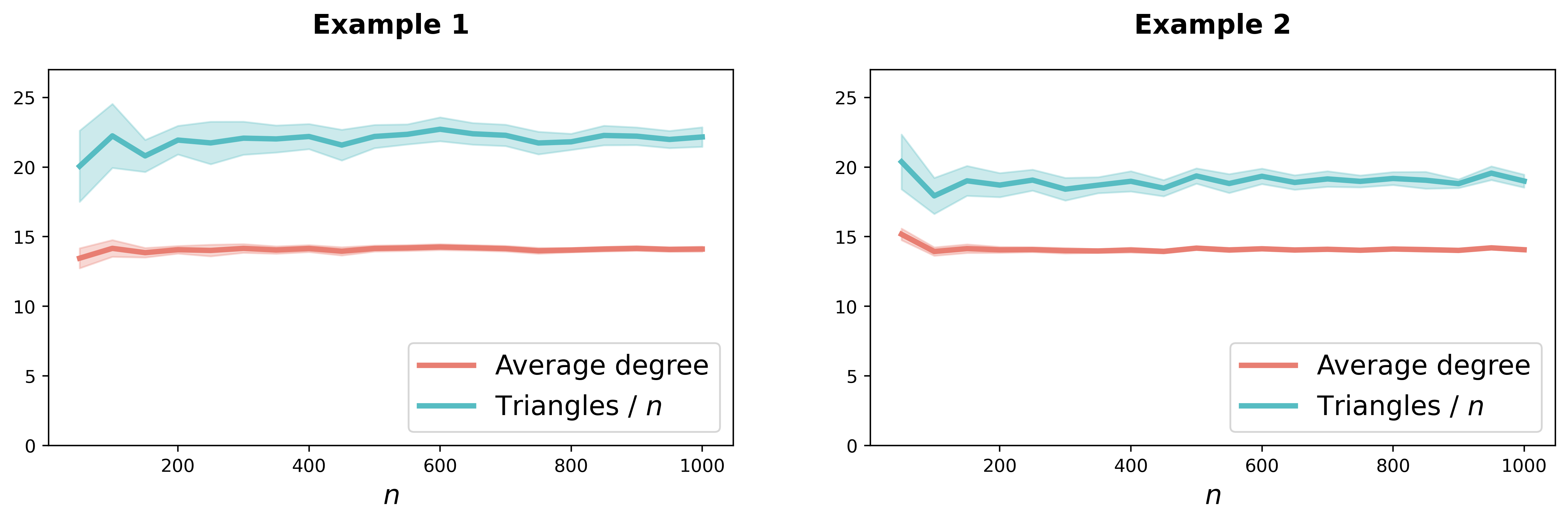
Seshadhri et al., 2020 note that for various real-world graphs, when looking only at the subgraphs containing nodes of maximum degree , they get a value of (in many cases ). Hence, we choose values of and (that are ) in our examples, which produce graphs of average degree in the same range. Figure 6 shows that setting and gives average degrees in this range and average for varying values of . The figure also illustrates that and stay (close to) constant as varies.
To show that the values of and do not vary too greatly over different simulations of graphs from the same model, Figures 7 and 8 show 100 samples from each model, again with and . We see that the average values (red line) correspond well to the values seen for varying in Figure 6.


A.13 Simulations of further examples
To illustrate that our results apply to models other than the two that we prove theoretically, in this section we present similar results from simulations of further models.
Example (3). Let , be the radial basis function (RBF) and be the uniform distribution on .
We show through simulations that if we let , then we get constant average degree and constant triangle density. This is illustrated in Figure 9 by simulating graphs from the model for increasing with .

Example (4). Let , be the radial basis function (RBF) and be the uniform distribution on .
We show through simulations that if we let , then we get constant average degree and constant triangle density. This is illustrated in Figure 10 by simulating graphs from the model for increasing with with .

A.14 Logistic model
Chanpuriya et al., 2020 propose a latent position model that they find is able to reconstruct sparse, triangle-dense graphs, where link probabilities are given by the logistic function,
As mentioned in the introduction, the effect of allowing two latent positions per node is complex, and not crucial for reproducing high triangle density. We therefore opt to present the manifold associated with the kernel above, rather than the asymmetric version in Chanpuriya et al., 2020. Figure 11 shows the first three dimensions of the manifold implicit in this kernel with a uniform latent position distribution (red curve) and the (Procrustes aligned) spectral embedding of a graph generated from it (blue points). The kernel is distortive (as one might expect, given it was never chosen not to be) and so the intrinsic (on-manifold) distribution is not uniform.

A.15 Neighbourhood approximations
Here we will demonstrate that the ‘number of shared neighbours’ metric forms a reasonable surrogate for the theoretical neighbourhood described in Section 3 (local embedding). The approximate neighbourhood around an arbitrary query node, , is found by taking the nodes with most neighbours in common with .
To investigate this hypothesis, we simulated a number of graphs from the model in Example (3) (Appendix A.13), with and so that the levels of sparsity and triangle density are in the range of real-world networks. As well as the shared neighbours metric, we also find an approximate neighbourhood based on the graph distance between nodes, i.e. the number of edges in the shortest path between nodes. Figure 12 shows the Jaccard similarity between the approximate neighbourhoods and the theoretical neighbourhood (nodes with latent positions closest to the latent position of the query node), where the Jaccard similarity between two sets and is defined as:
We see that the shared neighbours metric gives reasonable approximations to the theoretical neighbourhood for neighbourhoods of size between 5-15% of the size of the full graph.
