Bayesian Hyperbolic Multidimensional Scaling
Abstract
Multidimensional scaling (MDS) is a widely used approach to representing high-dimensional, dependent data. MDS works by assigning each observation a location on a low-dimensional geometric manifold, with distance on the manifold representing similarity. We propose a Bayesian approach to multidimensional scaling when the low-dimensional manifold is hyperbolic. Using hyperbolic space facilitates representing tree-like structures common in many settings (e.g. text or genetic data with hierarchical structure). A Bayesian approach provides regularization that minimizes the impact of measurement error in the observed data and assesses uncertainty. We also propose a case-control likelihood approximation that allows for efficient sampling from the posterior distribution in larger data settings, reducing computational complexity from approximately to . We evaluate the proposed method against state-of-the-art alternatives using simulations, canonical reference datasets, Indian village network data, and human gene expression data. Code to reproduce the result in the paper is available at https://github.com/peterliu599/BHMDS.
Keywords: Bayesian methods, Hyperbolic geometry, Multidimensional scaling
1 Introduction
Multidimensional scaling (MDS) methods represent high-dimensional data in a low-dimensional space, using dissimilarities between the observations as a means of identifying positions (Kruskal 1964). Observations with small dissimilarities will be placed close together, while those with larger dissimilarities will be placed further apart. A long literature on MDS methodology illustrates the utility of MDS as a means of summarizing complex, dependent data and for downstream applications, such as detecting clusters from the dissimilarities (Borg and Groenen 1997; Davison 1983; Cox and Cox 2001).
In many settings, the observed dissimilarities we wish to apply MDS methods to are likely to contain measurement error. These errors could arise from misreporting in the context of the social sciences (e.g. a retrospective behavioral inventory) or from miscalibration of machinery or operator error in industrial settings. Using a probabilistic model is one way to account for this additional uncertainty. Takane and Caroll 1981; Groenen 1993; MacKay 1989 and others have proposed maximum likelihood MDS methods for handling measurement error. The use of these methods relies on asymptotic theory, which might not apply to sample sizes used in applications, and the problem requires solving a non-linear optimization problem where the number of parameters grows quickly as the sample size grows (Cox and Cox 2001). One potential framework to address these potential issues with MDS is a Bayesian framework. Oh and Raftery 2001 provided a Bayesian procedure to estimate the configuration of objects given (potentially noisy) dissimilarities between objects. Extensions of Bayesian MDS to the case of large datasets were discussed in Holbrook et al. 2021.
Along with the statistical framework, another critical, but often ignored, choice in implementing MDS is the choice of geometry for the low-dimensional manifold. Multidimensional scaling methods often assume the observed dissimilarities are computed using Euclidean distances among objects in a Euclidean space. Oh and Raftery 2001, for example, assume a Euclidean distance model with a Gaussian measurement error and propose a Markov-Chain Monte Carlo algorithm to compute a Bayesian solution for the object configuration. Yet there is a growing literature showing that representing objects in other embedding spaces might lead to better representations and therefore be more useful in downstream tasks (De Sa et al. 2018; Chami et al. 2020; Smith et al. 2019; Lubold et al. 2020; Keller-Ressel and Nargang 2020). In particular, hyperbolic spaces, defined in Section 3, have been shown to produce embeddings with lower distortion, especially for data that is hierarchical or tree-like.
In this work, we combine the hyperbolic MDS methods with a Bayesian procedure. Specifically, we apply the Bayesian MDS procedure from Oh and Raftery 2001 to a hyperbolic space. Our model posits that the objects of interest are located in positions on a low-dimensional hyperbolic space, with the true dissimilarities between objects being the hyperbolic distances between positions. We further assume that the observed dissimilarities are the true dissimilarities plus a Gaussian error. We then derive a Markov-chain Monte Carlo (MCMC) method we use to obtain Bayesian estimates of the object positions, which allows practitioners to calculate distance-based measures (e.g. distances between positions, distances to the hyperbolic origin, etc.) that are often the pragmatic goals in applications.
The paper is organized as follows. In Section 3, we formally define the Hyperbolic space model used in this work and posit a model for observed dissimilarities computed from points in Hyperbolic space. We then discuss a prior distribution over this space and derive an MCMC algorithm to draw samples from the posterior in Section . Sections and contain simulations and applications of our method to real datasets in genomics. We conclude in Section 4.
2 Hyperbolic Geometry
We now discuss the mathematical details of the hyperbolic geometry. The hyperbolic geometry is a non-Euclidean geometry that has a constant negative curvature and is commonly visualized as the upper sheet of the unit two-sheet hyperboloid. There exist multiple equivalent hyperbolic models, such as the Klein model, the Poincaré disk model, and the Lorentz (Hyperboloid/Minkowski) model. We use the Lorentz model to parameterize the hyperbolic geometry, which parallels the representation used in existing hyperbolic MDS algorithms (Keller-Ressel and Nargang 2020; De Sa et al. 2018). This representation also facilitates convenient priors for our Bayesian model in Section 3.
To define the Lorentz model, we begin with the definition of the Lorentzian product. For any and , the Lorentzian product is defined as
The -dimensional Lorentz model with curvature , which we denote by , can be represented as a collection of coordinates with such that its Lorentzian product with itself is and equipped with the hyperbolic distance proportional to the square root of . That is,
equipped with the hyperbolic distance
| (1) |
which is the geodesic distance between and on . Specifically, the curvature controls the hyperbolicity of the geometry so that the space becomes more hyperbolic as becomes more negative and becomes flatter as shrinks to zero (Euclidean geometry has curvature exactly 0).
3 Bayesian Modeling Framework
We now describe our statistical framework for Bayesian Hyperbolic Multidimensional Scaling (BHMDS), which represents the objects of interest by coordinates in hyperbolic geometry, so that the hyperbolic distances between objects resemble their true dissimilarity measures. We suppose the objects dwell on with coordinates , and denote by the dissimilarity measure between object and object as well as the hyperbolic distance between and :
| (2) |
In many settings, the observed dissimilarities contain measurement errors. As in Oh and Raftery 2001, we represent the observed dissimilarity as the true dissimilarity plus a Gaussian error, with the constraint that the observed dissimilarity is always positive. We therefore assume that follows a truncated normal distribution:
| (3) |
where is as defined in (2), are unobserved, and is the variance of the measurement error.
Given the statistical model, we now specify priors for and . First note that, using (3), the likelihood of the unknown parameters and is
| (4) |
imal choice. Yet from numerical experiments and later applications, we find that the residuals fitted from the shortest path lengths closely follow a Gaussian distribution. We therefore conclude that the Gaussian error model works well with shortest path lengths as dissimilarities. Given the observed dissimilarity matrices, we fix the hyperbolic dimension as and estimate their curvature ’s as described in Appendix B, except for the karate dataset, where we set as in Keller-Ressel and Nargang 2020. Given the hyperbolic curvature and dimension, we use our BHMDS algorithm to compute the posterior estimate and the corresponding goodness-of-fit criteria. To compare the embedding performance with existing methods, we included results from common hyperbolic MDS methods using the same hyperbolic curvature and dimension, as well as Euclidean MDS methods with dimension .The embedding results are displayed in Table 1 and 2. We can conclude from the tables that the BHMDS algorithm attains optimal or close-to-optimal embedding in terms of both criteria on all four datasets. This indicates that, when the dissimilarity data are tree-like or hierarchical, the proposed BHMDS algorithm not only quantifies the uncertainty in the observed dissimilarity data but also embeds them into hyperbolic geometry with minimal information loss compared to the state-of-the-art MDS algorithms.
| Size | BHMDS | hydraPlus | hydra | BMDS | smacof | cmds | |
|---|---|---|---|---|---|---|---|
| Karate | 34 | 0.1780 | 0.1727 | 0.2105 | 0.2050 | 0.2112 | 0.2850 |
| Phylo | 344 | 0.0413 | 0.0413 | 0.2091 | 0.1601 | 0.1594 | 0.2481 |
| CS phd | 1025 | 0.1469 | 0.1471 | 0.2029 | 0.2281 | 0.2351 | 0.3862 |
| Wordnet | 1141 | 0.0798 | 0.0807 | 0.1279 | 0.2722 | 0.2725 | 0.4928 |
| Size | BHMDS | hydraPlus | hydra | BMDS | smacof | cmds | |
|---|---|---|---|---|---|---|---|
| Karate | 34 | 0.3485 | 0.3287 | 0.4278 | 0.3986 | 0.3742 | 0.5234 |
| Phylo | 344 | 0.1214 | 0.1206 | 0.6806 | 0.3552 | 0.3516 | 0.5918 |
| CS phd | 1025 | 0.2869 | 0.2868 | 0.4545 | 0.4523 | 0.4510 | 0.7513 |
| Wordnet | 1141 | 0.1441 | 0.1460 | 0.2242 | 0.4994 | 0.4967 | 0.9670 |
3.1 Approximated Log-likelihood: A Case Study
In this section, we present a case study to exemplify how to apply the stratified case-control log-likelihood and evaluate the algorithm’s likelihood precision and computational efficiency. We consider the WordNet mammals subtree dataset, a hierarchical NLP hypernym dataset studied by Nickel and Kiela 2017, as the input dataset. The WordNet dataset is in the form of an undirected graph with nodes, and we take the shortest path lengths on the graph between objects and as the observed dissimilarities . We set the hyperbolic dimension and estimate the curvature using the methods described in Appendix B.We now explain how to apply the approximated log-likelihood to the WordNet dataset. For each object , we first partition objects by their observed dissimilarity ’s. Since we are using the shortest path length as dissimilarity, all ’s are positive integers ranging from for each , and objects with the same value are in the same group. That is, we set
| (5) |
so that we collect all objects of distance to object in .We consider and , the two strata defined with the smallest dissimilarities (neighbors and second-neighbors) as cases and all other for as controls. We choose a control-to-case rate so that in the approximated log-likelihood, we explicitly calculate over of the terms in the exact likelihood. We run a pilot MCMC with 3,000 iterations, of which the first 1,000 are discarded as burn-in, to compute the relative weights and sample sizes for each for . We then run the case-control approximated log-likelihood MCMC to obtain the posterior estimate .We first evaluate the overall estimation performance of the case-control MCMC algorithm in terms of the stress and computation time. We run both the approximate and full MCMC algorithm with the WordNet dataset, and record the stress value of their posterior estimates as well as the computational times per 100 MCMC iterations. The results are shown in Table 3. We observe that the case-control approximate log-likelihood MCMC achieves comparable stress to the full MCMC but with only half of the computation time, indicating that the approximate MCMC achieves fast and accurate estimates of the true dissimilarities for large datasets.To evaluate the precision of the case-control likelihood, we compare the case-control log-likelihood change to the full log-likelihood change in the MCMC proposal of . If the case-control log-likelihood change approximates the full log-likelihood change well, the case-control MCMC will accept or reject in a similar pattern as the full MCMC. Recall that the change in the log-likelihood, as defined in Section , is.For a valid comparison, it is essential to evaluate both likelihood changes with respect to the same proposal and parameters such as . To this end, we first run the full MCMC algorithm with the Wordnet dataset, and record 100 sets of parameters from 100 MCMC iterations. For computational efficiency, we randomly sample 100 objects from the samples for each and make a proposal upon the corresponding under . We compute the approximate likelihood change and the full likelihood change for each proposal , and plot the approximated log-likelihood change values against the full log-likelihood change values in Figure 1. We observe that the approximate log-likelihood change is tightly aligned around , with a strongly positive correlation . This indicates the log-likelihood values computed from the proposed case-control MCMC algorithm are a good approximation to the true log-likelihood values. Furthermore, the case-control MCMC shares a similar accept/reject pattern as the full MCMC and is able to properly sample from the posterior.

| Method | hydraPlus | Approx | Full |
|---|---|---|---|
| Stress | 0.081 | 0.085 | 0.080 |
| MCMC time (100 iters) | - | 28.39s | 54.88s |
3.2 Assessing Network Centrality With BHMDS
We now use BHMDS to identify high-centrality nodes in a social network. Network centrality measures how centrally a node or actor is positioned in the network (Okamoto et al. 2008). Various centrality measures have been developed to describe the relative importance of a node in the network, such as degree centrality, closeness centrality, betweenness centrality, and eigenvector centrality (Koschützki et al. 2005). Centrality is useful in social and economic analysis. Among others, Bavelas 1950 shows that recognized leaders will most likely emerge at positions with a high closeness centrality of closeness. Banerjee et al. 2013 show that actors with a high eigenvector centrality facilitate the spread of information.In this example, we focus on closeness centrality, which is defined as the inverse of the average shortest path length from a given node to all other nodes in the network. By definition, the higher the closeness centrality, more proximate a node is to all other nodes on average. We claim that when using the shortest path lengths as dissimilarities to embed networks on hyperbolic space, the distance from the origin to a node’s embedded hyperbolic coordinates resembles the node’s closeness centrality. Similar centrality results are also reported in Turker and Balcisoy 2013 and Stai et al. 2016. Nodes that exhibit relatively equal and short distances to all other nodes can be interpreted as being located in the higher hierarchy of the network, so that by the nature of the hyperbolic geometry, it will be more likely to be embedded around the hyperbolic origin. Similarly, nodes that are relatively far from all the other nodes are more likely to be embedded far from the origin. This characteristic enables hyperbolic MDS methods to effectively assess network closeness.
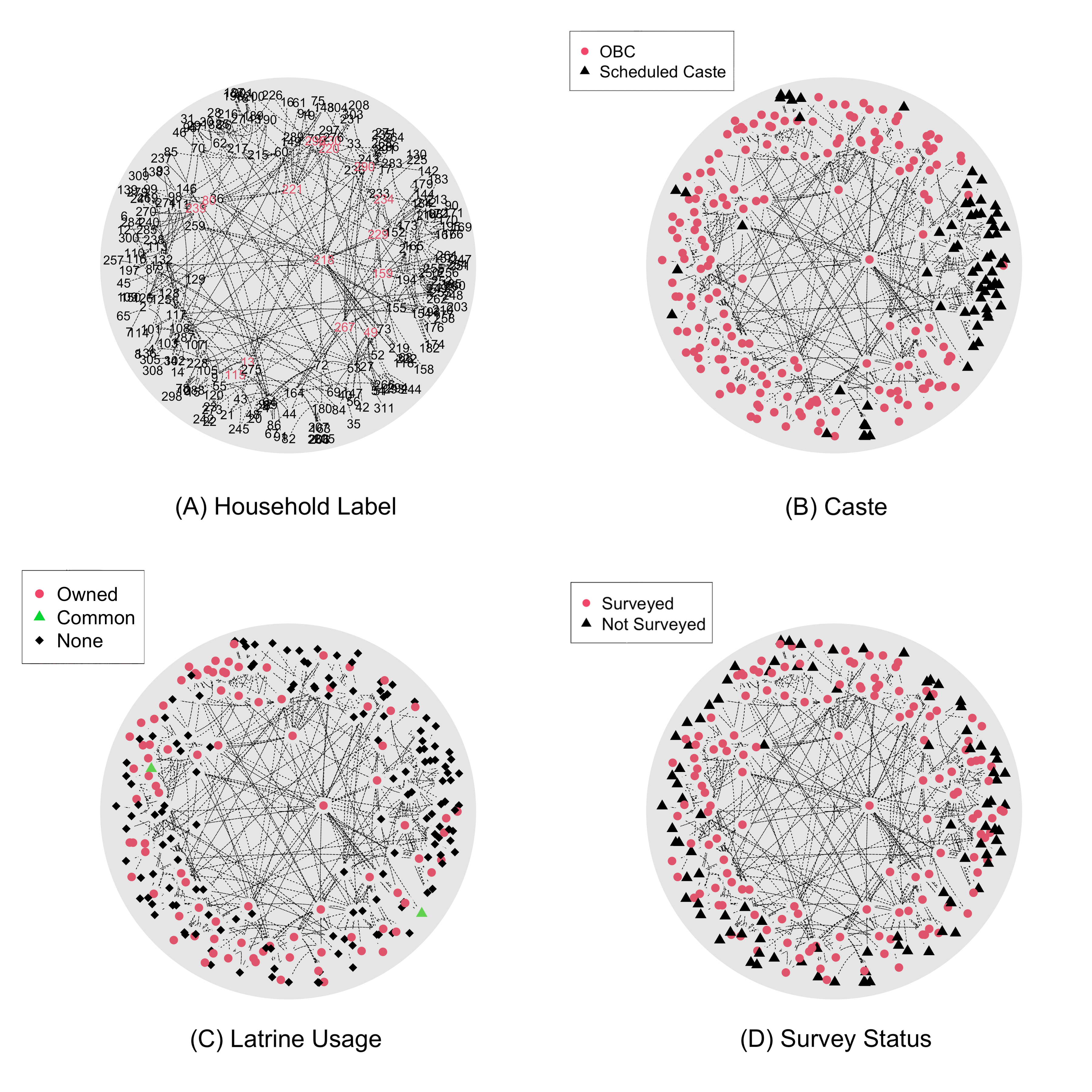

We apply BHMDS to financial networks from villages in rural India. The connections in these networks represent borrowing behaviors. Our goal is to access network closeness with uncertainty quantification and visualization. The network is collected by Banerjee et al. 2013 and describes the relationship of borrowing money between 248 households in a rural area of southern Karnataka, India. A household census, along with demographic covariates such as caste, religion, latrine usage, survey status, etc., is also collected. We use a public release of these data that contains a sample of households and can be found in https://dataverse.harvard.edu/dataset.xhtml?persistentId=doi:10.7910/DVN/U3BIHX. We first visualize the BHMDS embedding on the Poincaré disk in Figure 2 to identify potential nodes with high closeness and to observe the relations between covariates. For an optimal visualization layout, we first set . From (A), we observe that Households 218, 221, and 267 are among the closest to the origin, which also has the largest closeness centrality in the network. From (B) and (C), we observe a distinct cluster of households of scheduled caste on the right side of the disk, which systematically do not own a latrine. Moreover, in (D), we observe that households that do not participate in the survey appear at the edge of the disk. The ties between the unsurveyed households are mostly recorded from the surveyed households, and the ties between the unsurveyed households are missing.To further quantify the uncertainty in network centrality, we first run BHMDS repeatedly over a curvature interval and find that the stress is minimized with . Using this curvature, we run BHMDS again and record all MCMC samples of each node’s distance to the hyperbolic origin. Here, the optimal curvature is large, which potentially complicates the likelihood surface and makes optimization algorithms such as hydraPlus unstable. Specifically, it usually takes hydraPlus more than 60,000 iterations to converge, and households closest to the origin recognized by hydraPlus are not consistent across different trials. In contrast, even though using inconsistent hydraPlus as starting values, BHMDS consistently embeds the households with the highest closeness centrality the closest to the origin and achieves better stress than hydraPlus. Furthermore, in Figure 3 we observe that Households 218, 221, and 267 are distinctly closer to the origin. For all other nodes, although there is a gradient in the medians, the boxplots of their MCMC samples overlap significantly. Such uncertainty in the samples suggests that the centrality of these households is close and should be considered homogeneously. Together, these results suggest that BHMDS has some advantages over hydraPlus for this dataset.
,489.2025ptspspsp
3.3 Quantifying Uncertainty in Human Gene Expression Data
We now use the proposed BHMDS algorithm to analyze a global human gene expression dataset. Lukk et al. 2010 integrated microarray data from 5372 human samples representing 369 different cells & tissue types, disease states, and cell lines, and constructed a global human gene expression map. The original data come in the form of a gene expression matrix of over 22000 probe sets times 5372 genes of 15 human cell types.The expression matrix is jointly normalized by sample and library size, so that we can directly construct the dissimilarity matrix using the pairwise Euclidean distance of the gene vectors.Although the dissimilarities are computed from a Euclidean embedding, Zhou and Sharpee 2021 proposed that the intrinsic geometry of the human gene expression data is hyperbolic. Moreover, Elowitz et al. 2002, Oleksiak et al. 2002, and Raj and Oudenaarden 2008 argued that gene expression data are likely to contain measurement error. Together, these considerations motivate us to apply BHMDS with the human gene expression dissimilarity matrix to quantify the uncertainty in the data. Specifically, we use the case-control approximate MCMC algorithm to compute the Bayesian estimate of the cluster distances between cell type communities and quantify the uncertainty on the rank statistics of cell types’ evolution pseudotimes.We first elaborate on the details of the implementation of the case-control approximated MCMC. As the dissimilarity matrix is computed from high dimensional Euclidean metrics, the original human gene expression dissimilarities are large, which leads to overflow issues in computation. Thus, we preprocess the dissimilarity data as follows. We fix the hyperbolic curvature to , scale the dissimilarity matrix by a constant, and use hydraPlus to compute the corresponding stress with the hyperbolic dimension as chosen in Zhou and Sharpee 2021. We repeat the above process with a grid search over the scaling constants until we find an optimal constant. Such a process is similar in spirit to the algorithm described in Section B, as altering the curvature is roughly equivalent to scaling the distance as observed in (1), with the relationships between the dissimilarities unchanged. We found that scaling the dissimilarity by 10 yields the optimal stress at 0.046, resulting in a rescaled matrix with an average dissimilarity at 15.12. Since the dissimilarity in gene expression is continuous, we partition the rescaled dissimilarity by continuous intervals , and consider the dissimilarities that fall within as the case group. We choose , so that we will explicitly compute of the likelihood terms.To compute the Bayesian estimate of the cell type cluster distance, at each MCMC iteration, we record the cluster distance for cell type community and of size and as
| (6) |
where the community membership is given in the original data. We then take the posterior median of each , and plot them in Figure 4.Our Bayesian estimate identifies hematopoietic cells as distinct from all other cells, which is also observed in Lukk et al. 2010. We also observe modularity in neoplasm cells in the upper right corner of Heatmap 4, indicating their proximity in terms of evolutionary distance.

We further used the BHMDS algorithm to measure different cell types’ cellular differentiation using rank statistics with uncertainty quantification, a feature that is not available from previous methods used to analyze these data. Cellular differentiation refers to the transition of immature cells into specialized types, which is a central task in modern developmental biology (Klimovskaia et al. 2020). Specifically, Klimovskaia et al. 2020 studied the hierarchy of the single-cell data on hyperbolic geometry.For cells that are less differentiated, or at the beginning of a developmental process, they will be at the root of the evolutionary hierarchy and have relatively equal and small distances from all other cells, so that by the nature of the hyperbolic geometry, they are more likely to be embedded around the hyperbolic origin. Similarly, for cells that are more differentiated, they will have relatively large distances from all other cells, so they are more likely to be embedded distant from the origin. Thus, Klimovskaia et al. 2020 proposed that the hyperbolic distance between the origin and the cell’s embedded coordinate can be a good measure of the extent of the cell’s cellular differentiation, which they denoted as hyperbolic evolution pseudotime.In our study, at each MCMC iteration, we record the sampled evolution pseudotime for each gene and use them to construct the posterior credible intervals of the evolution pseudotime for each gene. To visualize the average evolution pseudotime for each cell type, we summarized the rank statistics of each cell type as follows. For each cell type community, we randomly sample one of its genes and draw from its nominal pseudotime confidence interval based on the posterior. Then, we rank the pseudotime drawn from each cell type community and record their rank statistics. We repeat the above process 10,000 times. We then summarize the rank statistics by frequency in Figure 5, where the -th entry of the heatmap represents the frequency of cell type being the -th closest to the hyperbolic origin, which indicates it is the -th least differentiated.Figure 5 indicates that cell types within the same cluster in Figure 4 share a similar hierarchy, as the neoplasm cells obtain higher frequency for the higher rank statistics and thus are less differentiated, whereas the hematopoietic cells yield higher frequency for the lower rank statistics, and thus are more differentiated. Additionally, we observe that the germ cell neoplasm has the smallest evolution pseudotime, entailed by the breast cancer cell. These results further shed light on the study of cancer stem cells, as short evolution pseudotimes of the two neoplasm cells suggest they are likely to be less differentiated or more de-differentiated, a phenomenon often observed in malignant tumors.

4 Conclusion
We have proposed a Bayesian approach to multidimensional scaling in hyperbolic space. Using a previously studied generating process for observed dissimilarities from Oh and Raftery 2001, we used prior distributions on hyperbolic space to derive the posterior distribution of the model parameters. We then proposed an MCMC procedure to sample from this posterior and also proposed a quick case-control method to efficiently sample from the posterior when the size of the observed dissimilarity matrix is large. Finally, we applied our methods to datasets in several domains and showed how our Bayesian procedure leads to embeddings with low distortion and allows us to quantify the uncertainty due to noise in the observed dissimilarities.The proposed method uses a state-of-the-art method called hydraPlus to choose parameters of the prior distribution and initialize the MCMC sampler. The major distinction between BHMDS and hydraPlus is that BHMDS quantifies the uncertainty in the dissimilarity data, which often leads to analyses that are more precise. Specifically, in Section 3.2, we show that BHMDS outperformed hydraPlus in some example datasets in identifying social network nodes with high closeness centrality using the extra uncertainty assessment. Through numerical experiments, we also find BHMDS often achieves better stress and gives stable estimates than hydraPlus when the sample size, hyperbolic curvature, or measurement error is large. Together this suggests that BHMDS numerically outperforms hydraPlus while adding to uncertainty quantification.In independent work issued just as we submitted this paper, Praturu andSharpee 2022 also carried out a Bayesian analysis of hyperbolic MDS. The present paper builds on Liu et al. 2022. The present work differs from that of Praturu andSharpee 2022 in several ways. Namely, we use priors for the latent positions in the hyperbolic space whereas Praturu andSharpee 2022 assume a Gaussian noise structure on distances. We choose to use priors on the positions as we consider a hyperbolic wrapped normal prior that allows us to reparameterize the posterior likelihood and greatly facilitate the MCMC sampler. Additionally, we propose using a case-control approximation to address computation whereas Praturu andSharpee 2022 use an iterative approach that adds observations in blocks.There are several potential avenues of future research. First, we have assumed in this work a low dimension for the desired embedding. While this does allow for easy visualization of the resulting embedding, imposing a low dimension on the dissimilarities is likely to lead to higher distortion than higher dimensions. One potential area of future work could derive an information criterion to estimate an optimal embedding dimension given the dissimilarities, as was done in Oh and Raftery 2001. A second possible direction is to explore how our proposed procedure could be adopted into the non-metric multidimensional scaling framework. Finally, while hyperbolic space has received considerable attention in the past few years, spaces of non-constant curvature, as studied in De Sa et al. 2018 and others, might lead to an embedding with lower distortions. An interesting research question here could focus on proposing Bayesian MDS methods in these spaces.
References
- Banerjee et al. (2013) A. Banerjee, A. G. Chandrasekhar, E. Duflo, and M. O. Jackson. The diffusion of microfinance. Science, 341(6144):1236498, 2013.
- Bavelas (1950) A. Bavelas. Communication patterns in task‐oriented groups. Journal of the Acoustical Society of America, 22:725–730, 111950.
- Borg and Groenen (1997) I. Borg and P. Groenen. Modern Multidimensional Scaling. New York: Springer-Verlag, 1997.
- Chami et al. (2020) I. Chami, A. Wolf, D.-C. Juan, F. Sala, S. Ravi, and C. Ré. Low-dimensional hyperbolic knowledge graph embeddings. arXiv preprint arXiv: 2005.00545, 01 2020.
- Cox and Cox (2001) T. F. Cox and M. A. A. Cox. Multidimensional Scaling. London: Chapman Hall, 2001.
- Davison (1983) M. L. Davison. Multidimensional Scaling. New York: Wiley, 1983.
- De Sa et al. (2018) C. De Sa, A. Gu, C. Ré, and F. Sala. Representation tradeoffs for hyperbolic embeddings. Proceedings of Machine Learning Research, 80, 04 2018.
- Doreian (2006) P. Doreian. Exploratory social network analysis with Pajek, W. de nooy, A.Mrvar, V. Batagelj. Cambridge University Press, New York(2005). Social Networks, 28:269–274, 07 2006.
- Elowitz et al. (2002) M. Elowitz, A. Levine, E. Siggia, and P. Swain. Stochastic gene expression in a single cell. Science (New York, N.Y.), 297:1183–6, 09 2002.
- Fonseca et al. (2012) T. Fonseca, H. Migon, and M. Ferreira. Bayesian analysis based on the jeffreys prior for the hyperbolicdistribution. Brazilian Journal of Probability and Statistics, 26, 11 2012.
- Gneiting et al. (2007) T. Gneiting, F. Balabdaoui, and A. Raftery. Probabilistic forecasts, calibration and sharpness. Journal of the Royal Statistical Society: Series B (StatisticalMethodology), 69:243 – 268, 04 2007.
- Groenen (1993) P. J. F. Groenen. The Majorization Approach to Multidimensional Scaling: SomeProblems and Extensions. Liden, The Netherlands: DSWO, 1993.
- Hofbauer et al. (2016) W. Hofbauer, L. Forrest, P. Hollingsworth, and M. Hart. Preliminary insights from DNA barcoding into the diversity ofmosses colonising modern building surfaces. Bryophyte Diversity and Evolution, 38:1, 04 2016.
- Hoff et al. (2002) P. D. Hoff, A. E. Raftery, and M. S. Handcock. Latent space approaches to social network analysis. Journal of the American Statistical Association, 2002.
- Holbrook et al. (2021) A. J. Holbrook, P. Lemey, G. Baele, S. Dellicour, D. Brockmann, A. Rambaut, andM. A. Suchard. Massive parallelization boosts big Bayesian multidimensionalscaling. Journal of Computational and Graphical Statistics, 30:11–24,2021.
- Keller-Ressel and Nargang (2020) M. Keller-Ressel and S. Nargang. Hydra: a method for strain-minimizing hyperbolic embedding ofnetwork- and distance-based data. Journal of Complex Networks, 8, 02 2020.
- Klimovskaia et al. (2020) A. Klimovskaia, D. Lopez-Paz, L. Bottou, and M. Nickel. Poincaré maps for analyzing complex hierarchies in single-cell data. Nature Communications, 11, 06 2020.
- Koschützki et al. (2005) D. Koschützki, K. A. Lehmann, L. Peeters, S. Richter, D. Tenfelde-Podehl,and O. Zlotowski. Centrality Indices, pages 16–61. Springer Berlin Heidelberg, Berlin, Heidelberg, 2005.
- Kruskal (1964) J. B. Kruskal. Multidimensional scaling by optimizing goodness of fit to a nonmetrichypothesis. Psychometrika, 29(1):1–27, 1964.
- Liu et al. (2022) B. Liu, S. Lubold, A. Raftery, and T. McCormick. Bayesian hyperbolic multidimensional scaling. Presentation at the Joint Statistical Meetings, Washington,D.C., August 2022.
- Lubold et al. (2020) S. Lubold, A. Chandrasekhar, and T. McCormick. Identifying the latent space geometry of network models throughanalysis of curvature. arXiv preprint arXiv:2012.10559, 2020.
- Lukk et al. (2010) M. Lukk, M. Kapushesky, J. Nikkilä, H. Parkinson, A. Goncalves, W. Huber,E. Ukkonen, and A. Brazma. A global map of human gene expression. Nature Biotechnology, 28:322–4, 04 2010.
- MacKay (1989) D. MacKay. Probabilistic multidimensional scaling: An anisotropic model fordistance judgements. Marketing Science, 5:325–334, 1989.
- Nagano et al. (2019) Y. Nagano, S. Yamaguchi, Y. Fujita, and M. Koyama. A wrapped normal distribution on hyperbolic space for gradient-basedlearning. arXiv preprint arXiv: 1902.02992, 2019.
- Nickel and Kiela (2017) M. Nickel and D. Kiela. Poincaré embeddings for learning hierarchical representations. arXiv preprint arXiv: 1705.08039, 05 2017.
- Oh and Raftery (2001) M.-S. Oh and A. E. Raftery. Bayesian multidimensional scaling and choice of dimension. Journal of the American Statistical Association,96(455):1031–1044, 2001.
- Okamoto et al. (2008) K. Okamoto, W. Chen, and X.-Y. Li. Ranking of closeness centrality for large-scale social networks. volume 5059, pages 186–195, 06 2008.
- Oleksiak et al. (2002) M. Oleksiak, G. Churchill, and D. Crawford. Variation in gene expression within and among natural populations. Nature Genetics, 32:261–6, 11 2002.
- Plummer et al. (2006) M. Plummer, N. Best, K. Cowles, and K. Vines. CODA: Convergence diagnosis and output analysis for MCMC. R News, 6(1):7–11, 2006.
- Praturu andSharpee (2022) A. Praturu and T. Sharpee. A Bayesian approach to hyperbolic multi-dimensional scaling. bioRxiv, 2022.
- Raftery andLewis (1992) A. E. Raftery and S. M. Lewis. Comment: one long run with diagnostics: implementation strategies forMarkov chain Monte Carlo. Statistical science, 7(4):493–497, 1992.
- Raftery et al. (2012) A. Raftery, X. Niu, P. Hoff, and K. Y. Yeung. Fast inference for the latent space network model using acase-control approximate likelihood. Journal of Computational and Graphical Statistics, 21, 10 2012.
- Raj and Oudenaarden (2008) A. Raj and A. Oudenaarden. Nature, nurture, or chance: Stochastic gene expression and itsconsequences. Cell, 135:216–26, 11 2008.
- Smith et al. (2019) A. L. Smith, D. M. Asta, C. A. Calder, et al. The geometry of continuous latent space models for network data. Statistical Science, 34(3):428–453, 2019.
- Stai et al. (2016) E. Stai, V. Karyotis, and S. Papavassiliou. A hyperbolic space analytics framework for big network data and theirapplications. IEEE Network, 30(1):11–17, 2016.
- Takane and Caroll (1981) Y. Takane and J. D. Caroll. Nonmetric maximum likelihood multidimensional scaling fromdirectional rankings of similarities. Psychometrika, 46:389–405, 1981.
- Turker and Balcisoy (2013) U. Turker and S. Balcisoy. A visualization technique for large temporal social network datasetsin hyperbolic space. Journal of Visual Languages & Computing, 25, 01 2013.
- Zachary (1976) W. Zachary. An information flow model for conflict and fission in small groups. Journal of anthropological research, 33, 11 1976.
- Zhou and Sharpee (2021) Y. Zhou and T. Sharpee. Hyperbolic geometry of gene expression. iScience, 24:102225, 02 2021.
Appendix A Reasoning of the Prior Choice
Note that, since each is defined on , we cannot apply a usual multivariate normal prior on as in Oh and Raftery 2001, which is originally defined on the Euclidean geometry. It is tempting to consider distributions defined on the hyperbolic space as substitutes of the multivariate normal distribution, such as the distributions described in Fonseca et al. 2012 and Nagano et al. 2019, and directly specify the prior on . However, since the hyperbolic space is centered around instead of the Euclidean origin , directly impose a hyperbolic prior on will generally lead to an asymmetric proposal function, and restrict us from applying the random walk Metropolis-Hastings sampling algorithm described in Oh and Raftery 2001, which uses a symmetric proposal function, and is more tractable and computationally efficient.
Appendix B Curvature Estimation through Stress Minimization
In this section, we define an estimate of the curvature of the given (potentially) noisy dissimilarities between points on . An advantage of the estimator we now propose is that it does not depend on knowing the dimension of the space. For any curvature value , we let for denote the set of embedding coordinates obtained from BHMDS or hydraPlus computed using the curvature value , and we let be the distance between and . Our estimate is then the estimate that minimizes the stress between the observed dissimilarities and the distances . That is, we set
In general, we find BHMDS yields better curvature estimates than hydraPlus, thus we recommend using BHMDS for curvature estimation if computation power permits.This is not the only way to estimate the curvature of given (potentially) noisy dissimilarity data. Lubold et al. 2020, for example, proposed a different estimate of curvature and proved it is consistent as the error in goes to zero. But we found in simulations that the above estimator outperforms the estimate in Lubold et al. 2020 for the noise levels we consider in this work.
Appendix C Identifiability and Hyperbolic Visualization
In general, hyperbolic visualization refers to representing objects around the center of an (often) two-dimensional Poincare disk. Yet, due to the nature of hyperbolic space, the volume of hyperbolic space is not constant from the origin, and it is possible to transform the hyperbolic coordinates through Procrustean operations and represent the objects using only part of the Poincare disk, with the distances between coordinates to be invariant. One may refer to Klimovskaia et al. 2020 for more detail. This suggests there is no unique way in visualizing hyperbolic data.In BHMDS, we consider a hyperbolic wrapped normal distribution centered at the hyperbolic origin as the prior of the coordinates. Such a prior choice indicates we attempt to embed objects at the center of the hyperbolic space. Specifically, BHMDS will try to embed objects with equal and small distances to all others around the hyperbolic origin and to embed objects with large distances to others away.Technically, our Bayesian estimate of is not precisely centered at the origin as specified in the prior. A set of is said to be centered at the origin if its inverse transformation on the Euclidean space has mean zero and diagonal covariance matrix. In Euclidean MDS, it is possible to center the Euclidean coordinates by Procrustean operation (see postprocessing in Oh and Raftery 2001). In the hyperbolic space, we cannot use Procrustean operations on to center , as the transformation is not invariant to Procrustean operations so that the distances are not preserved after centering . Still, from simulations and the network example in the newly added Section 3.2, BHMDS consistently embed objects by their distances to the origin and identifies nodes with high centrality. This suggests BHMDS embeds as theoretically expected.In other applications, practitioners identify a certain object as the root of structure. For instance, in genomic study, embryonic stem cells can be viewed as the root of the differentiation process. The choices of root are often subjective to expertise knowledge, so that visualization is highly customized and changes with respect to different choices of the root. Klimovskaia et al. 2020 describes a transformation that centers the hyperbolic coordinates by setting the root object at the hyperbolic origin while preserving the hyperbolic distances. Practitioners can use such transformation to recenter the BHMDS estimate accordingly for visualization.Thus, if the goal is to identify nodes that is central and close to all others, we may directly visualize the BHMDS result on the Poincare disk, as in Section 3.2. Otherwise, one will need to transform the estimates before visualization as in Klimovskaia et al. 2020.Additionally, when the coordinates are centered with respect to the root, their distances to the origin will change accordingly. This suggests that, if the distances to the origins are of practical interest, we need to postprocess the MCMC samples by the transformation before calculating the distances to the origin. In the example in 3.3, we have not identified a cell type that is commonly recognized as the root of differentiation, but we still observe the more de-differentiated breast cancer cell and the less differentiated germ cell neoplasm embedded around the hyperbolic origin. This indicates postprocessing is not necessary in the example.
Appendix D MCMC Convergence
In this section, we provide typical trace plots from our simulations and data sets. We plot the MCMC proposed and values over iterations for the MCMC simulation in Section . Specifically, to comprehensively investigate the convergence of , we ran a BHMDS simulation for sample size , hyperbolic dimension , error size , with 20,000 MCMC iterations and burn-in of 3,000 iterations, randomly pick ten entries from the dissimilarity matrix, and record their MCMC sampled values after the MCMC burn-in. We provide the trace plots below. We also assessed convergence using the diagnostic of Raftery andLewis 1992. We analyze the traces using the default raftery.diag() function from the coda R package (Plummer et al. 2006), and summarize the results in Table 4. Our choice of the total number of MCMC iterations is close to the average of the suggested total number of MCMC iterations, iterations . This suggests that around 20,000 MCMC iterations are enough to estimate the parameters of interest in BHMDS.

| Burn-in (M) | Total (N) | Lower bound (Nmin) | Dependence factor (I) | |
|---|---|---|---|---|
| Sample 1 | 21 | 24222 | 3746 | 6.47 |
| Sample 2 | 18 | 19083 | 3746 | 5.09 |
| Sample 3 | 18 | 20487 | 3746 | 5.47 |
| Sample 4 | 24 | 24474 | 3746 | 6.53 |
| Sample 5 | 20 | 22194 | 3746 | 5.92 |
| Sample 6 | 18 | 20061 | 3746 | 5.36 |
| Sample 7 | 18 | 21762 | 3746 | 5.81 |
| Sample 8 | 20 | 22152 | 3746 | 5.91 |
| Sample 9 | 20 | 23348 | 3746 | 6.23 |
| Sample 10 | 18 | 21612 | 3746 | 5.77 |
| 18 | 18158 | 3746 | 4.85 |