Learning to predict arbitrary quantum processes
Abstract
We present an efficient machine learning (ML) algorithm for predicting any unknown quantum process over qubits. For a wide range of distributions on arbitrary -qubit states, we show that this ML algorithm can learn to predict any local property of the output from the unknown process , with a small average error over input states drawn from . The ML algorithm is computationally efficient even when the unknown process is a quantum circuit with exponentially many gates. Our algorithm combines efficient procedures for learning properties of an unknown state and for learning a low-degree approximation to an unknown observable. The analysis hinges on proving new norm inequalities, including a quantum analogue of the classical Bohnenblust-Hille inequality, which we derive by giving an improved algorithm for optimizing local Hamiltonians. Numerical experiments on predicting quantum dynamics with evolution time up to and system size up to qubits corroborate our proof. Overall, our results highlight the potential for ML models to predict the output of complex quantum dynamics much faster than the time needed to run the process itself.
I Introduction
Learning complex quantum dynamics is a fundamental problem at the intersection of machine learning (ML) and quantum physics. Given an unknown -qubit completely positive trace preserving (CPTP) map that represents a physical process happening in nature or in a laboratory, we consider the task of learning to predict functions of the form
| (1) |
where is an -qubit state and is an -qubit observable. Related problems arise in many fields of research, including quantum machine learning biamonte2017quantum; schuld2019quantum; havlivcek2019supervised; caro2022generalization; schreiber2022classical; mcclean2018barren; caro2022out; huang2022quantum; farhi2018classification; arunachalam2017guest, variational quantum algorithms gibbs2022dynamical; cirstoiu2020variational; peruzzo2014variational; kandala2017hardware; kokail2019self; cerezo2021variational; grimsley2019adaptive, machine learning for quantum physics carleo2017solving; sharir2020deep; van2017learning; zhou2017optimizing; carrasquilla2017machine; parr1980density; car1985unified; becke1993new; white1993density; gilmer2017neural; huang2021provably; huang2020power, and quantum benchmarking mohseni2008quantum; Scott08; o2004quantum; levy2021classical; huang2022foundations; merkel2013self; blume2017demonstration. As an example, for predicting outcomes of quantum experiments huang2021information; melnikov2018active; huang2022quantum, we consider to be parameterized by a classical input , is an unknown process happening in the lab, and is an observable measured at the end of the experiment. Another example is when we want to use a quantum ML algorithm to learn a model of a complex quantum evolution with the hope that the learned model can be faster cirstoiu2020variational; gibbs2022dynamical; caro2022out.
As an -qubit CPTP map consists of exponentially many parameters, prior works, including those based on covering number bounds caro2022generalization; caro2022out; huang2021information; huang2022quantum, classical shadow tomography levy2021classical; kunjummen2021shadow, or quantum process tomography mohseni2008quantum; Scott08; o2004quantum, require an exponential number of data samples to guarantee a small constant error for predicting outcomes of an arbitrary evolution under a general input state . To improve upon this, recent works chung2019sample; caro2022generalization; caro2022out; huang2021information; huang2022quantum have considered quantum processes that can be generated in polynomial-time and shown that a polynomial amount of data samples suffices to learn in this restricted class. However, these results still require exponential computation time.
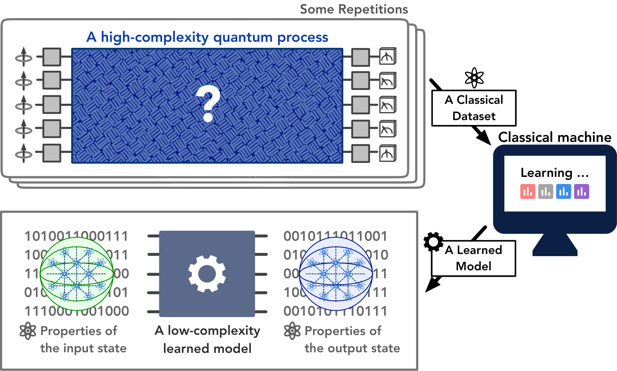
In this work, we present a computationally-efficient ML algorithm that can learn a model of an arbitrary unknown -qubit process , such that given sampled from a wide range of distributions over arbitrary -qubit states and any in a large physically-relevant class of observables, the ML algorithm can accurately predict . The ML model can predict outcomes for highly entangled states after learning from a training set that only contains data for random product input states and randomized Pauli measurements on the corresponding output states. The training and prediction of the proposed ML model are both efficient even if the unknown process is a Hamiltonian evolution over an exponentially long time, a quantum circuit with exponentially many gates, or a quantum process arising from contact with an infinitely large environment for an arbitrarily long time. Furthermore, given few-body reduced density matrices (RDMs) of the input state , the ML algorithm uses only classical computation to predict output properties .
The proposed ML model is a combination of efficient ML algorithms for two learning problems: (1) predicting given a known observable and an unknown state , and (2) predicting given an unknown observable and a known state . We give sample- and computationally-efficient learning algorithms for both problems. Then we show how to combine the two learning algorithms to address the problem of learning to predict for an arbitrary unknown -qubit quantum process . Together, the sample and computational efficiency of the two learning algorithms implies the efficiency of the combined ML algorithm.
In order to establish the rigorous guarantee for the proposed ML algorithms, we consider a different task: optimizing a -local Hamiltonian . We present an improved approximate optimization algorithm that finds either a maximizing/minimizing state with a rigorous lower/upper bound guarantee on the energy in terms of the Pauli coefficients of . The rigorous bounds improve upon existing results on optimizing -local Hamiltonians Dinur2006OnTF; barak_et_al:LIPIcs:2015:5298; harrow2017extremal; anshu2021improved. We then use the improved optimization algorithm to give a constructive proof of several useful norm inequalities relating the spectral norm of an observable and the -norm of the Pauli coefficients associated to the observable . The proof resolves a recent conjecture in RWZ2022KKL about the existence of quantum Bohnenblust-Hille inequalities. These norm inequalities are then used to establish the efficiency of the proposed ML algorithms.
II Learning quantum states, observables, and processes
Before proceeding to state our main results in greater detail, we describe informally the learning tasks discussed in this paper: what do we mean by learning a quantum state, observable, and process?
II.1 Learning an unknown state
It is possible in principle to provide a complete classical description of an -qubit quantum state . However this would require an exponential number of experiments, which is not at all practical. Therefore, we set a more modest goal: to learn enough about to predict many of its physically relevant properties. We specify a family of target observables and a small target accuracy . The learning procedure is judged to be successful if we can predict the expectation value of every observable in the family with error no larger than .
Suppose that is an arbitrary and unknown -qubit quantum state, and suppose that we have access to identical copies of . We acquire information about by measuring these copies. In principle, we could consider performing collective measurements across many copies at once. Or we might perform single-copy measurements sequentially and adaptively; that is, the choice of measurement performed on copy could depend on the outcomes obtained in measurements on copies The target observables we consider are bounded-degree observables. A bounded-degree -qubit observable is a sum of local observables (each with support on a constant number of qubits independent of ) such that only a constant number (independent of ) of terms in the sum act on each qubit. Most thermodynamic quantities that arise in quantum many-body physics can be written as a bounded-degree observable , such as a geometrically-local Hamiltonian or the average magnetization.
In the learning protocols discussed in this paper, the measurements are neither collective nor adaptive. Instead, we fix an ensemble of possible single-copy measurements, and for each copy of we independently sample from this ensemble and perform the selected measurement on that copy. Thus there are two sources of randomness in the protocol — the randomly chosen measurement on each copy, and the intrinsic randomness of the quantum measurement outcomes. If we are unlucky, the chosen measurements and/or the measurement outcomes might not be sufficiently informative to allow accurate predictions. We will settle for a protocol that achieves the desired prediction task with a high success probability.
For the protocol to be practical, it is highly advantageous for the sampled measurements to be easy to perform in the laboratory, and easy to describe in classical language. The measurements we consider, random Pauli measurements, meet both of these criteria. For each copy of and for each of the qubits, we choose uniformly at random to measure one of the three single-qubit Pauli observables , , or . This learning method, called classical shadow tomography, was analyzed in huang2020predicting, where an upper bound on the sample complexity (the number of copies of needed to achieve the task) was expressed in terms of a quantity called the shadow norm of the target observables.
In this work, using a new norm inequality derived here, we improve on the result in huang2020predicting by obtaining a tighter upper bound on the shadow norm for bounded degree observables. The upshot is that, for a fixed target accuracy , we can predict all bounded-degree observables with spectral norm less than by performing random Pauli measurement on
| (2) |
copies of . This result improves upon the previously known bound of . Furthermore, we derive a matching lower bound on the number of copies required for this task, which applies even if collective measurements across many copies are allowed.
II.2 Learning an unknown observable
Now suppose that is an arbitrary and unknown -qubit observable. We also consider a distribution on -qubit quantum states. This distribution, too, need not be known, and it may include highly entangled states. Our goal is to find a function which predicts the expectation value of the observable on the state with a small mean squared error:
To define this learning task, it is convenient to assume that we can access training data of the form
| (3) |
where is sampled from the distribution . In practice, though, we cannot directly access the exact value of the expectation value ; instead, we might measure multiple times in the state to obtain an accurate estimate of the expectation value. Furthermore, we don’t necessarily need to sample states from to achieve the task. We might prefer to learn about by accessing its expectation value in states drawn from a different ensemble.
A crucial idea of this work is that we can learn efficiently if the distribution has suitably nice features. Specifically, we consider distributions that are invariant under single-qubit Clifford gates applied to any one of the qubits. We say that such distributions are locally flat, meaning that the probability weight assigned to an -qubit state is unmodified (i.e., the distribution appears flat) when we locally rotate any one of the qubits.
An arbitrary observable can be expanded in terms of the Pauli operator basis:
| (4) |
Though there are Pauli operators, if the distribution is locally flat and has a constant spectral norm, we can approximate the sum over by a truncated sum
| (5) |
including only the Pauli operators with weight up to , those acting nontrivially on no more than qubits. The mean squared error incurred by this truncation decays exponentially with . Therefore, to learn with mean squared error it suffices to learn this truncated approximation to , where . Furthermore, using norm inequalities derived in this paper, we show that for the purpose of predicting the expectation value of this truncated operator it suffices to learn only a few relatively large coefficients , while setting the rest to zero. The upshot is that, for a fixed target error , an observable with constant spectral norm can be learned from training data with size , where the classical computational cost of training and predicting is .
Usually, in machine learning, after learning from a training set sampled from a distribution , we can only predict new instances sampled from the same distribution . We find, though, that for the purpose of learning an unknown observable, there is a particular locally flat distribution such that learning to predict under suffices for predicting under any other locally flat distribution. Namely, we samples from the -qubit state distribution by preparing each one of the qubits in one of the six Pauli operator eigenstates , chosen uniformly at random. Pleasingly, preparing samples from is not only sufficient for our task, but also easy to do with existing quantum devices.
After training is completed, to predict for a new state drawn from the distribution , we need to know some information about . The state , like the operator , can be expanded in terms of Pauli operators, and when we replace by its weight- truncation, only the truncated part of contributes to its expectation value. Thus if the -body reduced density matrices (RDMs) for states drawn from are known classically, then the predictions can be computed classically. If the states drawn from are presented as unknown quantum states, then we can learn these -body RDMs efficiently (for small ) using classical shadow tomography, and then proceed with the classical computation to obtain a predicted value of .
II.3 Learning an unknown process
Now suppose that is an arbitrary and unknown quantum process mapping qubits to qubits. Let be a family of target observables, and be a distribution on quantum states. We assume the ability to repeatedly access for a total of times. Each time we can apply to an input state of our choice, and perform the measurement of our choice on the resulting output. In principle we could allow input states that are entangled across the channel uses, and allow collective measurements across the channel outputs. But here we confine our attention to the case where the inputs are unentangled, and the channel outputs are measured individually. Our goal is to find a function which predicts, with a small mean squared error, the expectation value of in the output state for every observable in the family :
| (6) |
Our main result is that this task can be achieved efficiently if is a bounded-degree observable and is locally flat. That is, , the number of times we access , and the computational complexity of training and prediction, scale reasonably with the system size and the target accuracy .
To prove this result, we observe that the task of learning an unknown quantum process can be reduced to learning unknown states and learning unknown observables. If is sampled from the distribution , then, since is unknown, should be regarded as an unknown quantum state. Suppose we learn this state; that is, after preparing and measuring sufficiently many times we can accurately predict the expectation value for each target observable .
Now notice that , where is the (Heisenberg-picture) map dual to . Since is unknown, should be regarded as an unknown observable. Suppose we learn this observable; that is, using the dataset as training data, we can predict for drawn from with a small mean squared error. This achieves the task of learning the process for state distribution and target observable .
Having already shown that arbitrary quantum states can be learned efficiently for the purpose of predicting expectation values of bounded-degree observables, and that arbitrary observables can be learned efficiently for locally flat input state distributions, we obtain our main result. Since the distribution is locally flat, it suffices to learn the low-degree truncated approximation to the unknown operator , incurring only a small mean squared error. To predict , then, it suffices to know only the few-body RDMs of the input state . For any input state , these few-body density matrices can be learned efficiently using classical shadow tomography.
As noted above in the discussion of learning observables, the states in the training data need not be sampled from . To learn a low-degree approximation to , it suffices to sample from a locally flat distribution on product states. Even if we sample only product states during training, we can make accurate predictions for highly entangled input states. We also emphasize again that the unknown process is arbitrary. Even if has quantum computational complexity exponential in , we can learn to predict accurately and efficiently, for bounded-degree observables and for any locally flat distribution on the input state .
III Algorithm for learning an unknown quantum process
Consider an unknown -qubit quantum process (a CPTP map). Suppose we have obtained a classical dataset by performing randomized experiments on . Each experiment prepares a random product state , passes through , and performs a randomized Pauli measurement huang2020predicting; elben2022randomized on the output state. Recall that a randomized Pauli measurement measures each qubit of a state in a random Pauli basis (, or ) and produces a measurement outcome of , where . We denote the classical dataset of size to be
| (7) |
where . Each product state is represented classically with bits. Hence, the classical dataset is of size bits. The classical dataset can be seen as one way to generalize the notion of classical shadows of quantum states huang2020predicting to quantum processes. Our goal is to design an ML algorithm that can learn an approximate model of from the classical dataset , such that for a wide range of states and observables , the ML model can predict a real value that is approximately equal to .
III.1 ML algorithm
We are now ready to state the proposed ML algorithm. At a high level, the ML algorithm learns a low-degree approximation to the unknown -qubit CPTP map . Despite the simplicity of the ML algorithm, several ideas go into the design of the ML algorithm and the proof of the rigorous performance guarantee. These ideas are presented in Section IV.
Let be an observable with that is written as a sum of few-body observables, where each qubit is acted by of the few-body observables. We denote the Pauli representation of as . By definition of , there are nonzero Pauli coefficients . We consider a hyperparameter ; roughly speaking will scale inverse polynomially in the dataset size from Eq. (12). For every Pauli observable with , the algorithm computes an empirical estimate for the corresponding Pauli coefficient via
| (8) | ||||
| (9) |
The computation of and can both be done classically. The basic idea of is to set the coefficient to zero when the influence of Pauli observable is negligible. Given an -qubit state , the algorithm outputs
| (10) |
With a proper implementation, the computational time is . Note that, to make predictions, the ML algorithm only needs the -body reduced density matrices (-RDMs) of . The -RDMs of can be efficiently obtained by performing randomized Pauli measurement on and using the classical shadow formalism huang2020predicting; elben2022randomized. Except for this step, which may require quantum computation, all other steps of the ML algorithm only requires classical computation. Hence, if the -RDMs of can be computed classically, then we have a classical ML algorithm that can predict an arbitrary quantum process after learning from data.
III.2 Rigorous guarantee
To measure the prediction error of the ML model, we consider the average-case prediction performance under an arbitrary -qubit state distribution invariant under single-qubit Clifford gates, which means that the probability distribution of sampling a state is equal to of sampling for any single-qubit Clifford gate . We call such a distribution locally flat.
Theorem 1 (Learning an unknown quantum process).
Given and a training set of size as specified in Eq. (7). With high probability, the ML model can learn a function from such that for any distribution over -qubit states invariant under single-qubit Clifford gates, and for any bounded-degree observable with ,
| (11) |
where is the low-degree truncation (of degree ) of the observable after the Heisenberg evolution under . The training and prediction time of are both polynomial in . When is small and , the data size and computational time scale as .
The detailed theorem statement and the proof of the theorem are given in Appendix E. An interesting aspect of the above theorem is that the states sampled from the distribution can be highly entangled, even though the training data only contains information about random product states. From the theorem, we can see that if , then we only need samples to obtain a constant prediction error. Otherwise, samples is still enough to guarantee a constant prediction error relative to . The precise scaling is given as follows. Consider data size
| (12) |
The computational time to learn and predict is bounded above by and the prediction error is bounded as
| (13) |
As we take to be zero, we can remove the dependence on the low-degree truncation . In this setting, and computation time both become , which is polynomial in if .
IV Proof ideas
The proof of the rigorous performance guarantee for the proposed ML algorithm consists of five parts. The first two parts presented in Appendix A and Appendix B are a detour to establish a few fundamental and useful norm inequalities about Hamiltonians/observables. The latter three parts given in Appendix C, Appendix D, and Appendix E apply the newly-established norm inequalities to three learning tasks. In the following, we present the basic ideas in each part.
IV.1 Improved approximation algorithms for optimizing local Hamiltonians
We begin with a different task, namely optimizing local Hamiltonians. We are given an -qubit -local Hamiltonian
| (14) |
where is the weight of the Pauli operator , the number of qubits upon which acts nontrivially. Our goal is to find a state that maximizes/minimizes . This task is related to solving ground states kempe2006complexity; sakurai_napolitano_2017 when we consider minimizing and quantum optimization farhi2014quantum; Farhi2014AQA; harrow2017extremal; parekh2020beating; Hallgren2020AnAA; anshu2021improved; hastings2022optimizing when we consider maximizing .
We give a general randomized approximation algorithm in Appendix A for producing a random product state that either approximately minimizes or approximately maximizes a -local Hamiltonian with a rigorous upper/lower bound based on the Pauli coefficients of . The proposed optimization algorithm applies to various classes of Hamiltonians and is inspired by the proofs of Littlewood’s 4/3 inequality littlewood1930bounded and the Bohnenblust-Hille inequality BHineq1931. For classes that have been studied previously Dinur2006OnTF; barak_et_al:LIPIcs:2015:5298; harrow2017extremal; anshu2021improved, the proposed algorithm obtains an improved bound. Our improvement crucially stems from our construction for the random state . Dinur2006OnTF; barak_et_al:LIPIcs:2015:5298; harrow2017extremal utilize a random restriction approach, where some random subset of qubits are fixed with some random values and the rest of the qubits are optimized. On the other hand, we utilize a polarization approach, where we replicate each qubit many times, randomly fix all except the last replica, optimize the last replica, and combine using a random-signed averaging. A detailed comparison is given in Appendix A.1.3 and A.2.
Two classes of Hamiltonians used in our learning applications are general -local Hamiltonians and bounded-degree -local Hamiltonians. A -local Hamiltonian with degree at most is a Hermitian operator that can be written as a sum of -qubit observables, where each qubit is acted on by at most of the -qubit observables.
Corollary 1 (Optimizing general -local Hamiltonian).
Given an -qubit -local Hamiltonian
| (15) |
There is a randomized algorithm that runs in time and produces either a random maximizing state satisfying
| (16) |
or a random minimizing state satisfying
| (17) |
where .
Corollary 2 (Optimizing bounded-degree -local Hamiltonian).
Given an -qubit -local Hamiltonian with bounded degree , for all , and . There is a randomized algorithm that runs in time and produces either a random maximizing state satisfying
| (18) |
or a random minimizing state satisfying
| (19) |
for some constant .
We note that in the above results, we cannot control whether our algorithm outputs an approximate maximizer or minimizer. This caveat stems from the use of polarization, where the random-signed averaging only guarantees improvement in one of the two directions. Modifying our approach to address this issue is an interesting direction for future work.
IV.2 Norm inequalities from approximate optimization algorithms
The bridge that connects the optimization of -local Hamiltonians and efficient learning of quantum states and processes is a set of norm inequalites. A norm that characterizes the efficiency of learning is the Pauli- norm, defined as the -norm on the Pauli coefficients of an observable/Hamiltonian ,
| (20) |
The rigorous guarantees from the previous section, namely on finding a state whose energy is higher/lower than a Haar-random state by a margin that depends on the Pauli coefficients , give an algorithmic proof that the spectral norm and the Pauli coefficients are related. The proof of this relation is given in Appendix B. In particular, for general and bounded-degree -local Hamiltonian, we can use the rigorous guarantee from the approximation algorithms to obtain the following norm inequalites. Corollary 3 proves the conjecture given in RWZ2022KKL.
Corollary 3 (Norm inequality for general -local Hamiltonian).
Given an -qubit -local Hamiltonian . We have
| (21) |
where .
Corollary 4 (Norm inequality for bounded-degree local Hamiltonian).
Given an -qubit -local Hamiltonian with a bounded degree . We have
| (22) |
where .
IV.3 Sample-optimal algorithm for predicting bounded-degree observables
As the first application of the above norm inequalities to learning, we consider the basic problem of predicting many properties of an unknown -qubit state . Given observables , after performing measurements on multiple copies of , we would like to predict to error for all . This is the task known as shadow tomography aaronson2018shadow; aaronson2019gentle; huang2020predicting. One approach for obtaining practically-efficient algorithms for shadow tomography is via the classical shadow formalism huang2020predicting.
We consider a physically-relevant class of observables, where the observable is a sum of few-body observables and each qubit is acted on by of the few-body observables. Despite significant recent progress in shadow tomography levy2021classical; zhao2021fermionic; hu2021hamiltonian; koh2020classical; chen2020robust; hadfield2020measurements; aaronson2018shadow; struchalin2020experimental; huang2022learning; o2022fermionic; wan2022matchgate; bu2022classical; huang2022quantum; chen2022exponential; coopmans2022predicting, the sample complexity (number of copies of ) for predicting this class of observables has not been established. The central challenge is the appearance of the Pauli- norm when characterizing the sample complexity. In particular, one can bound the shadow norm huang2020predicting, which gives an upper bound on the sample complexity in terms of the Pauli- norm up to a constant factor. Using the new norm inequality established in this work, we give a sample-optimal algorithm for predicting bounded-degree observables.
The sample-optimal algorithm is equivalent to performing classical shadow tomography based on randomized Pauli measurements huang2020predicting; elben2022randomized, and is essentially the ML algorithm given in Section III.1 with a fixed input state. Consider an unknown -qubit state . After performing randomized Pauli measurements on copies of , we have a classical dataset denoted as
| (23) |
where is a single-qubit stabilizer state. Given an observable , the algorithm predicts
| (24) |
It is not hard to see that computing only requires classical computation time. Hence, as we show later that , the learning algorithm is very efficient. Using the norm inequality for bounded-degree local Hamiltonian for a constant in Corollary 4, and the classical shadow formalism huang2020predicting; elben2022randomized, we obtain the following performance guarantee.
Theorem 2 (Sample complexity upper bound).
Given an unknown -qubit state and any -qubit observables with . Suppose each observable is a sum of few-body observables, where each qubit is acted on by of the few-body observables. Using a classical dataset of size
| (25) |
we have with high probability. The constant factor in the notation above scales polynomially in the degree and exponentially in the locality of the observables.
The following theorem shows that the above algorithm achieves the optimal sample complexity among any algorithms that can perform collective measurement on many copies of .
Theorem 3 (Sample complexity lower bound).
Consider the following task. There is an unknown -qubit state , and we are given observables with . Each observable is a sum of few-body observables, where every qubit is acted on by of the few-body observables. We would like to estimate to error for all with high probability by performing arbitrary collective measurements on copies of . The number of copies must be at least
| (26) |
for any algorithm to succeed in this task.
The detailed proofs of the sample complexity stated in the above theorems are given in Appendix C.
IV.4 Efficient algorithms for learning an unknown observable from samples
As a second learning application of the norm inequalities, we consider the task of learning an unknown -qubit observable . We can think of this unknown observable as , i.e., the observable after Heisenberg evolution under the unknown process . Suppose we are given a training dataset of , where is sampled from an arbitrary distribution over -qubit states that is invariant under single-qubit Clifford gates. Given an integer , we define the weight- truncation of to be the following Hermitian operator
| (27) |
where is the number of qubits upon which acts nontrivially. For a small , we can think of as a low-weight approximation of the unknown observable . By definition, is a -local Hamiltonian, hence the norm inequality in Corollary 3 shows that
| (28) |
where . An norm bound () on the Pauli coefficients implies that we can remove most of the small Pauli coefficients without incurring too much change under the norm. As an example, consider an -dimensional vector with . Given , let be the -dimensional vector with if and if . We have
| (29) |
In Appendix D.1, we show that the average error (both the mean squared error and the mean absolute error) is characterized by the norm. Hence, Eq. (28) implies that we can set most of the Pauli coefficients in to zero without incurring too much error on average.
Using the above reasoning, learning the low-weight truncation amounts to learning the large Pauli coefficients of and setting all small Pauli coefficients to zero. This ensures that the learning can be done very efficiently. This approach is presented in Appendix D.2 with the main result stated in Lemma 18. It is inspired by the learning algorithm of eskenazis2022learning that achieves a logarithmic sample complexity for learning classical low-degree functions.
The last step in the proof is to argue that the low-weight truncation is a good surrogate for the unknown observable when the goal is to predict . The key insight here is that for distributions that are invariant under single-Clifford gates, the contribution of any Pauli term in to is exponentially decaying in the the weight . This allows us to prove that is small.
Putting these ingredients together, we arrive at the following theorem. As stated in the theorem, the learning algorithm is computationally efficient.
Theorem 4 (Learning an unknown observable).
Given . Let and . From training data of size
| (30) |
where is sampled from , we can learn a function such that
| (31) |
with probability at least . The training and prediction time of are .
The factor of in the prediction error is the natural scale of the squared error. From the theorem, we can see that we only need samples to obtain a constant prediction error relative to . The proof the the theorem and the detailed description of the ML algorithm are given in Appendix D.
IV.5 Learning an unknown quantum process
The ML algorithm for learning an unknown -qubit quantum process is essentially the combination of the two learning applications described above with a few modifications. At a high level, we consider the following. There is an -qubit state sampled from an unknown distribution , as well as an observable that can be written as a sum of few-body observables, where each qubit is acted on by a constant number of the few-body observables. In the first stage, we use the sample-optimal algorithm for predicting the bounded-degree observable , where is an unknown quantum state, thus transforming the classical dataset in Eq. (7) into a dataset,
| (32) |
that maps quantum states to real numbers. In the second stage, we apply the efficient algorithm for learning an unknown observable , regarding Eq. (32) as the training data for this task, thus predicting for the state drawn from the distribution . Because both stages of the algorithm run in time polynomial in , the overall runtime for this procedure is polynomial in .
In our actual proofs, there are a few deviations from the above high-level design, stemming from the fact that the input states are tensor products of random single-qubit stabilizer states. This specific setting allows a few simplifications to be made. With the simplifications, we can remove an additive factor of in the prediction error. Furthermore, a surprising fact is that learning from random product states is sufficient to predict highly-entangled states sampled from any distribution invariant under single-qubit Clifford unitaries. This surprising fact is a result of the characterization of the prediction error given in Lemma 14 based on a modified purity on subsystems of an input quantum state .
By combining the five parts together, we can establish Theorem 1, the precise sample complexity scaling in Eq. (12), and the prediction error bound in Eq. (13). The full proof is given in Appendix E.
V Numerical experiments
We have conducted numerical experiments to assess the performance of ML models in learning the dynamics of several physical systems. The results corroborate our theoretical claims that long-time evolution over a many-body system can be learned efficiently. While our theorem only guarantees good performance for randomly sampled input states, we also find that the ML models work very well for structured input states that could be of practical interest. The source code can be found on a public GitHub repository11 1 https://github.com/hsinyuan-huang/learning-quantum-process.
We focus on training ML models to predict output state properties after the time dynamics of 1D -spin XY/Ising chains with homogeneous/disordered fields. Let be the many-body Hamiltonian. The quantum processes is given by for a significantly long evolution time . We consider the ML models described by Eq. (10). While we utilize the very simple sparsity-enforcing strategy of setting small values to zero to prove Theorem 1, the standard sparsity-enforcing approach is through regularization tibshirani1996regression. A detailed description of applying regularization to enforce sparsity in is given in Appendix F. We find the best hyperparameters using four-fold cross-validation to minimize root-mean-square error (RMSE) and report the predictions on a test set.
Fig. 2 considers the performance for predicting the expectation of the Pauli-Z operator on the output state for randomly sampled product input states not in the training data. Fig. 2(a) illustrates the many-body Hamiltonian . Fig. 2(b) shows the dependence of the error on training set size . We can clearly see that as training set size increases, the prediction error notably decreases. This observation confirms our theoretical claim that long-time quantum dynamics could be efficiently learned. In Fig. 2(c), we consider how evolution time affects prediction performance. From the figure, we can see that even when we exponentially increase , the prediction performance remains similar. This matches with our theorem stating that no matter what the quantum process is, even if is an exponentially long-time dynamics, the ML model can still predict accurately and efficiently. In Fig. 2(d), we consider the dependence on system size . As increases linearly, the Hilbert space dimension grows exponentially. Despite the exponential growth, even for -spin systems, the ML model still predicts well. This matches with the logarithmic scaling on given in Theorem 1.
In Fig. 3, we consider predicting properties of the final state after long-time dynamics for a highly structured input product state:
| (33) |
which has a single domain wall in the middle. We focus on predicting the expected value for on every spin in the 1D 50-spin XY chain with a homogeneous field and consider evolution time from to . We train the ML model using random input product states. We can see that the ML model predicts very well for this highly structured product state. The collapse of the domain wall is accurately predicted by the ML model despite only seeing outcomes from random unstructured product states. This numerical experiment suggests that the performance of the ML model goes beyond Theorem 1, which only guarantees accurate prediction on average.
Theorem 1 states that the ML model can predict well on highly-entangled input states after learning only from random product state inputs. We test this claim in Fig. 4 by considering an entangled input state
| (34) |
The left spins of the state exhibit GHZ-like entanglement, which requires a linear-depth 1D quantum circuit to prepare. The right spins of form a product state with spins rotating clockwise from left to right. Combining the left and right spins together, the state cannot be generated by a short-depth 1D quantum circuit. We can see that for this entangled input state, the ML model trained on random product states still predicts very well across a broad range of the evolution time .
VI Outlook
The theorem established in this work shows that learning to predict a complex quantum process can be achieved with computationally-efficient ML algorithms. Once we have obtained training data by accessing the unknown process sufficiently many times, the proposed ML algorithm is entirely classical except for the step of obtaining the reduced density matrix (RDM) of the input state , which may require quantum computation. This algorithm is reminiscent of recent proposals for quantum ML based on kernel methods havlivcek2019supervised; schuld2019quantum; huang2020power, in particular the projected quantum kernel huang2020power. This result highlights the potential for using hybrid quantum-classical ML algorithms to learn to model exotic quantum dynamics occurring in nature.
The results presented in this work also have implications in several previously-studied problems. Prior works cirstoiu2020variational; gibbs2022dynamical; caro2022out have proposed to train quantum ML algorithms on a given quantum process with the hope that the learned model can be faster than the process itself. Our proof that even an exponential-time quantum dynamics can be predicted in quasi-polynomial time provides rigorous support for such a hope. Furthermore, the proposed ML algorithm can be efficiently run on a classical computer when the few-body RDMs of the input state is easy to compute classically. Hence, this result provides a rigorous foundation for empirical works using classical ML to learn and simulate quantum dynamics torlai2020quantum; gentile2021learning; banchi2018modelling; gilmer2017neural. When is a parameterized quantum circuit , such as a quantum neural network mcclean2018barren; caro2022generalization; havlivcek2019supervised; farhi2018classification; huang2020power; huang2021information, the existence of a classical ML model that can efficiently predict the output of implies that the function is easy to represent and learn on a classical computer. This finding shows that quantum circuits do not have strong representational power for a wide range of distributions over quantum state input with easy-to-compute RDMs.
Several open problems remain to be answered. While we only focus on locally flat distributions , we believe that efficient ML algorithms also exist for other general classes of distributions. An important open problem is hence the following: Can we obtain computationally efficient learning algorithms for any “smooth” distribution over quantum state space? If not, how general can the class of distributions be? Similar questions can be asked about the class of observables that we predict. For what general classes of observables can one predict efficiently, in terms of both sample size and computation time? This problem is closely related to the problem of when shadow tomography aaronson2018shadow; aaronson2019gentle; aaronson22shadow can be made computationally efficient. Other important questions include: If we restrict the quantum process to be generated in polynomial time, can we obtain improved efficiency? What efficiency guarantees apply to fermionic or bosonic systems? A better understanding of these problems would illuminate the ultimate power of classical and quantum ML algorithms for learning about physical dynamics.
Acknowledgements.
The authors thank Victor V. Albert, Chi-Fang (Anthony) Chen, Bryan Clark, Richard Kueng, and Spiros Michalakis for valuable input and inspiring discussions. After learning about our proof of the quantum Bohnenblust-Hille inequality, Alexander Volberg and Haonan Zhang found a very different proof with a better Bohnenblust-Hille constant. We thank them for sharing their results with us. HH is supported by a Google PhD fellowship. SC is supported by NSF Award 2103300. JP acknowledges funding from the U.S. Department of Energy Office of Science, Office of Advanced Scientific Computing Research, (DE-NA0003525, DE-SC0020290), and the National Science Foundation (PHY-1733907). The Institute for Quantum Information and Matter is an NSF Physics Frontiers Center.References
- [1] Jacob Biamonte, Peter Wittek, Nicola Pancotti, Patrick Rebentrost, Nathan Wiebe, and Seth Lloyd. Quantum machine learning. Nature, 549(7671):195–202, 2017.
- [2] Maria Schuld and Nathan Killoran. Quantum machine learning in feature hilbert spaces. Phys. Rev. Lett., 122(4):040504, 2019.
- [3] Vojtěch Havlíček, Antonio D Córcoles, Kristan Temme, Aram W Harrow, Abhinav Kandala, Jerry M Chow, and Jay M Gambetta. Supervised learning with quantum-enhanced feature spaces. Nature, 567(7747):209–212, 2019.
- [4] Matthias C Caro, Hsin-Yuan Huang, Marco Cerezo, Kunal Sharma, Andrew Sornborger, Lukasz Cincio, and Patrick J Coles. Generalization in quantum machine learning from few training data. Nature communications, 13(1):1–11, 2022.
- [5] Franz J Schreiber, Jens Eisert, and Johannes Jakob Meyer. Classical surrogates for quantum learning models. arXiv preprint arXiv:2206.11740, 2022.
- [6] Jarrod R McClean, Sergio Boixo, Vadim N Smelyanskiy, Ryan Babbush, and Hartmut Neven. Barren plateaus in quantum neural network training landscapes. Nature communications, 9(1):1–6, 2018.
- [7] Matthias C Caro, Hsin-Yuan Huang, Nicholas Ezzell, Joe Gibbs, Andrew T Sornborger, Lukasz Cincio, Patrick J Coles, and Zoë Holmes. Out-of-distribution generalization for learning quantum dynamics. arXiv preprint arXiv:2204.10268, 2022.
- [8] Hsin-Yuan Huang, Michael Broughton, Jordan Cotler, Sitan Chen, Jerry Li, Masoud Mohseni, Hartmut Neven, Ryan Babbush, Richard Kueng, John Preskill, et al. Quantum advantage in learning from experiments. Science, 376(6598):1182–1186, 2022.
- [9] Edward Farhi and Hartmut Neven. Classification with quantum neural networks on near term processors. arXiv preprint arXiv:1802.06002, 2018.
- [10] Srinivasan Arunachalam and Ronald de Wolf. Guest column: A survey of quantum learning theory. ACM SIGACT News, 48(2):41–67, 2017.
- [11] Joe Gibbs, Zoë Holmes, Matthias C Caro, Nicholas Ezzell, Hsin-Yuan Huang, Lukasz Cincio, Andrew T Sornborger, and Patrick J Coles. Dynamical simulation via quantum machine learning with provable generalization. arXiv preprint arXiv:2204.10269, 2022.
- [12] Cristina Cirstoiu, Zoe Holmes, Joseph Iosue, Lukasz Cincio, Patrick J Coles, and Andrew Sornborger. Variational fast forwarding for quantum simulation beyond the coherence time. npj Quantum Information, 6(1):1–10, 2020.
- [13] Alberto Peruzzo, Jarrod McClean, Peter Shadbolt, Man-Hong Yung, Xiao-Qi Zhou, Peter J Love, Alán Aspuru-Guzik, and Jeremy L O’brien. A variational eigenvalue solver on a photonic quantum processor. Nat. Commun., 5:4213, 2014.
- [14] Abhinav Kandala, Antonio Mezzacapo, Kristan Temme, Maika Takita, Markus Brink, Jerry M Chow, and Jay M Gambetta. Hardware-efficient variational quantum eigensolver for small molecules and quantum magnets. Nature, 549(7671):242–246, 2017.
- [15] Christian Kokail, Christine Maier, Rick van Bijnen, Tiff Brydges, Manoj K Joshi, Petar Jurcevic, Christine A Muschik, Pietro Silvi, Rainer Blatt, Christian F Roos, et al. Self-verifying variational quantum simulation of lattice models. Nature, 569(7756):355–360, 2019.
- [16] Marco Cerezo, Andrew Arrasmith, Ryan Babbush, Simon C Benjamin, Suguru Endo, Keisuke Fujii, Jarrod R McClean, Kosuke Mitarai, Xiao Yuan, Lukasz Cincio, et al. Variational quantum algorithms. Nature Reviews Physics, 3(9):625–644, 2021.
- [17] Harper R Grimsley, Sophia E Economou, Edwin Barnes, and Nicholas J Mayhall. An adaptive variational algorithm for exact molecular simulations on a quantum computer. Nat. Commun., 10(1):1–9, 2019.
- [18] Giuseppe Carleo and Matthias Troyer. Solving the quantum many-body problem with artificial neural networks. Science, 355(6325):602–606, 2017.
- [19] Or Sharir, Yoav Levine, Noam Wies, Giuseppe Carleo, and Amnon Shashua. Deep autoregressive models for the efficient variational simulation of many-body quantum systems. Phys. Rev. Lett., 124(2):020503, 2020.
- [20] Evert PL Van Nieuwenburg, Ye-Hua Liu, and Sebastian D Huber. Learning phase transitions by confusion. Nat. Phys., 13(5):435–439, 2017.
- [21] Zhenpeng Zhou, Xiaocheng Li, and Richard N Zare. Optimizing chemical reactions with deep reinforcement learning. ACS Cent. Sci., 3(12):1337–1344, 2017.
- [22] Juan Carrasquilla and Roger G Melko. Machine learning phases of matter. Nat. Phys., 13(5):431–434, 2017.
- [23] Robert G Parr. Density functional theory of atoms and molecules. In Horizons of quantum chemistry, pages 5–15. Springer, 1980.
- [24] Richard Car and Mark Parrinello. Unified approach for molecular dynamics and density-functional theory. Phys. Rev. Lett., 55(22):2471, 1985.
- [25] Axel D Becke. A new mixing of hartree–fock and local density-functional theories. J. Chem. Phys., 98(2):1372–1377, 1993.
- [26] Steven R White. Density-matrix algorithms for quantum renormalization groups. Phys. Rev. B, 48(14):10345, 1993.
- [27] Justin Gilmer, Samuel S Schoenholz, Patrick F Riley, Oriol Vinyals, and George E Dahl. Neural message passing for quantum chemistry. arXiv preprint arXiv:1704.01212, 2017.
- [28] Hsin-Yuan Huang, Richard Kueng, Giacomo Torlai, Victor V Albert, and John Preskill. Provably efficient machine learning for quantum many-body problems. arXiv preprint arXiv:2106.12627, 2021.
- [29] Hsin-Yuan Huang, Michael Broughton, Masoud Mohseni, Ryan Babbush, Sergio Boixo, Hartmut Neven, and Jarrod R McClean. Power of data in quantum machine learning. Nat. Commun., 12(1):1–9, 2021.
- [30] Masoud Mohseni, Ali T Rezakhani, and Daniel A Lidar. Quantum-process tomography: Resource analysis of different strategies. Phys. Rev. A, 77(3):032322, 2008.
- [31] A. J. Scott. Optimizing quantum process tomography with unitary 2-designs. J. Phys., A41:055308, 2008.
- [32] Jeremy L O’Brien, Geoff J Pryde, Alexei Gilchrist, Daniel FV James, Nathan K Langford, Timothy C Ralph, and Andrew G White. Quantum process tomography of a controlled-not gate. Physical review letters, 93(8):080502, 2004.
- [33] Ryan Levy, Di Luo, and Bryan K Clark. Classical shadows for quantum process tomography on near-term quantum computers. arXiv preprint arXiv:2110.02965, 2021.
- [34] Hsin-Yuan Huang, Steven T Flammia, and John Preskill. Foundations for learning from noisy quantum experiments. arXiv preprint arXiv:2204.13691, 2022.
- [35] Seth T Merkel, Jay M Gambetta, John A Smolin, Stefano Poletto, Antonio D Córcoles, Blake R Johnson, Colm A Ryan, and Matthias Steffen. Self-consistent quantum process tomography. Physical Review A, 87(6):062119, 2013.
- [36] Robin Blume-Kohout, John King Gamble, Erik Nielsen, Kenneth Rudinger, Jonathan Mizrahi, Kevin Fortier, and Peter Maunz. Demonstration of qubit operations below a rigorous fault tolerance threshold with gate set tomography. Nature communications, 8(1):1–13, 2017.
- [37] Hsin-Yuan Huang, Richard Kueng, and John Preskill. Information-theoretic bounds on quantum advantage in machine learning. Phys. Rev. Lett., 126:190505, 2021.
- [38] Alexey A Melnikov, Hendrik Poulsen Nautrup, Mario Krenn, Vedran Dunjko, Markus Tiersch, Anton Zeilinger, and Hans J Briegel. Active learning machine learns to create new quantum experiments. Proc. Natl. Acad. Sci. U.S.A., 115(6):1221–1226, 2018.
- [39] Jonathan Kunjummen, Minh C Tran, Daniel Carney, and Jacob M Taylor. Shadow process tomography of quantum channels. arXiv preprint arXiv:2110.03629, 2021.
- [40] Kai-Min Chung and Han-Hsuan Lin. Sample efficient algorithms for learning quantum channels in pac model and the approximate state discrimination problem. arXiv preprint arXiv:1810.10938, 2018.
- [41] Irit Dinur, Ehud Friedgut, Guy Kindler, and Ryan O’Donnell. On the fourier tails of bounded functions over the discrete cube. Israel Journal of Mathematics, 160:389–412, 2006.
- [42] Boaz Barak, Ankur Moitra, Ryan O’Donnell, Prasad Raghavendra, Oded Regev, David Steurer, Luca Trevisan, Aravindan Vijayaraghavan, David Witmer, and John Wright. Beating the Random Assignment on Constraint Satisfaction Problems of Bounded Degree. In Naveen Garg, Klaus Jansen, Anup Rao, and José D. P. Rolim, editors, Approximation, Randomization, and Combinatorial Optimization. Algorithms and Techniques (APPROX/RANDOM 2015), volume 40 of Leibniz International Proceedings in Informatics (LIPIcs), pages 110–123, Dagstuhl, Germany, 2015. Schloss Dagstuhl–Leibniz-Zentrum fuer Informatik.
- [43] Aram W Harrow and Ashley Montanaro. Extremal eigenvalues of local hamiltonians. Quantum, 1:6, 2017.
- [44] Anurag Anshu, David Gosset, Karen J Morenz Korol, and Mehdi Soleimanifar. Improved approximation algorithms for bounded-degree local hamiltonians. Physical Review Letters, 127(25):250502, 2021.
- [45] Cambyse Rouzé, Melchior Wirth, and Haonan Zhang. Quantum talagrand, kkl and friedgut’s theorems and the learnability of quantum boolean functions. 2022.
- [46] Hsin-Yuan Huang, Richard Kueng, and John Preskill. Predicting many properties of a quantum system from very few measurements. Nat. Phys., 16:1050––1057, 2020.
- [47] Andreas Elben, Steven T Flammia, Hsin-Yuan Huang, Richard Kueng, John Preskill, Benoît Vermersch, and Peter Zoller. The randomized measurement toolbox. arXiv preprint arXiv:2203.11374, 2022.
- [48] Julia Kempe, Alexei Kitaev, and Oded Regev. The complexity of the local hamiltonian problem. Siam journal on computing, 35(5):1070–1097, 2006.
- [49] J. J. Sakurai and Jim Napolitano. Modern Quantum Mechanics. Cambridge University Press, 2 edition, 2017.
- [50] Edward Farhi, Jeffrey Goldstone, and Sam Gutmann. A quantum approximate optimization algorithm. arXiv preprint arXiv:1411.4028, 2014.
- [51] Edward Farhi, Jeffrey Goldstone, and Sam Gutmann. A quantum approximate optimization algorithm applied to a bounded occurrence constraint problem. arXiv: Quantum Physics, 2014.
- [52] Ojas Parekh and Kevin Thompson. Beating random assignment for approximating quantum 2-local hamiltonian problems. arXiv preprint arXiv:2012.12347, 2020.
- [53] Sean Hallgren, Eun Young Lee, and Ojas Parekh. An approximation algorithm for the max-2-local hamiltonian problem. In APPROX-RANDOM, 2020.
- [54] Matthew B Hastings and Ryan O’Donnell. Optimizing strongly interacting fermionic hamiltonians. In Proceedings of the 54th Annual ACM SIGACT Symposium on Theory of Computing, pages 776–789, 2022.
- [55] John E Littlewood. On bounded bilinear forms in an infinite number of variables. The Quarterly Journal of Mathematics, (1):164–174, 1930.
- [56] H. F. Bohnenblust and Einar Hille. On the absolute convergence of dirichlet series. Annals of Mathematics, 32(3):600–622, 1931.
- [57] Scott Aaronson. Shadow tomography of quantum states. In STOC, pages 325–338, 2018.
- [58] Scott Aaronson and Guy N Rothblum. Gentle measurement of quantum states and differential privacy. In STOC, pages 322–333, 2019.
- [59] Andrew Zhao, Nicholas C Rubin, and Akimasa Miyake. Fermionic partial tomography via classical shadows. Physical Review Letters, 127(11):110504, 2021.
- [60] Hong-Ye Hu and Yi-Zhuang You. Hamiltonian-driven shadow tomography of quantum states. arXiv preprint arXiv:2102.10132, 2021.
- [61] Dax Enshan Koh and Sabee Grewal. Classical shadows with noise. arXiv preprint arXiv:2011.11580, 2020.
- [62] Senrui Chen, Wenjun Yu, Pei Zeng, and Steven T Flammia. Robust shadow estimation. arXiv preprint arXiv:2011.09636, 2020.
- [63] Charles Hadfield, Sergey Bravyi, Rudy Raymond, and Antonio Mezzacapo. Measurements of quantum hamiltonians with locally-biased classical shadows. arXiv:2006.15788, 2020.
- [64] GI Struchalin, Ya A Zagorovskii, EV Kovlakov, SS Straupe, and SP Kulik. Experimental estimation of quantum state properties from classical shadows. arXiv preprint arXiv:2008.05234, 2020.
- [65] Hsin-Yuan Huang. Learning quantum states from their classical shadows. Nature Reviews Physics, 4(2):81–81, 2022.
- [66] Bryan O’Gorman. Fermionic tomography and learning. arXiv preprint arXiv:2207.14787, 2022.
- [67] Kianna Wan, William J Huggins, Joonho Lee, and Ryan Babbush. Matchgate shadows for fermionic quantum simulation. arXiv preprint arXiv:2207.13723, 2022.
- [68] Kaifeng Bu, Dax Enshan Koh, Roy J Garcia, and Arthur Jaffe. Classical shadows with pauli-invariant unitary ensembles. arXiv preprint arXiv:2202.03272, 2022.
- [69] Sitan Chen, Jordan Cotler, Hsin-Yuan Huang, and Jerry Li. Exponential separations between learning with and without quantum memory. In 2021 IEEE 62nd Annual Symposium on Foundations of Computer Science (FOCS), pages 574–585. IEEE, 2022.
- [70] Luuk Coopmans, Yuta Kikuchi, and Marcello Benedetti. Predicting gibbs state expectation values with pure thermal shadows. arXiv preprint arXiv:2206.05302, 2022.
- [71] Alexandros Eskenazis and Paata Ivanisvili. Learning low-degree functions from a logarithmic number of random queries. In Proceedings of the 54th Annual ACM SIGACT Symposium on Theory of Computing, pages 203–207, 2022.
- [72] Robert Tibshirani. Regression shrinkage and selection via the lasso. Journal of the Royal Statistical Society: Series B (Methodological), 58(1):267–288, 1996.
- [73] Giacomo Torlai, Christopher J Wood, Atithi Acharya, Giuseppe Carleo, Juan Carrasquilla, and Leandro Aolita. Quantum process tomography with unsupervised learning and tensor networks. arXiv preprint arXiv:2006.02424, 2020.
- [74] Antonio A Gentile, Brian Flynn, Sebastian Knauer, Nathan Wiebe, Stefano Paesani, Christopher E Granade, John G Rarity, Raffaele Santagati, and Anthony Laing. Learning models of quantum systems from experiments. Nature Physics, 17(7):837–843, 2021.
- [75] Leonardo Banchi, Edward Grant, Andrea Rocchetto, and Simone Severini. Modelling non-markovian quantum processes with recurrent neural networks. New Journal of Physics, 20(12):123030, 2018.
- [76] Weiyuan Gong and Scott Aaronson. Learning distributions over quantum measurement outcomes. 2022.
- [77] Stephen Piddock and Ashley Montanaro. The complexity of antiferromagnetic interactions and 2d lattices. arXiv preprint arXiv:1506.04014, 2015.
- [78] Uffe Haagerup. The best constants in the khintchine inequality. Studia Mathematica, 70(3):231–283, 1981.
- [79] Peter Borwein and Tamás Erdélyi. Polynomials and polynomial inequalities, volume 161. Springer Science & Business Media, 1995.
- [80] L. LeCam. Convergence of estimates under dimensionality restrictions. The Annals of Statistics, 1(1):38–53, 1973.
- [81] Yihong Wu. Lecture notes on information-theoretic methods for high-dimensional statistics. Lecture Notes for ECE598YW (UIUC), 16, 2017.
- [82] Elliott Lieb, Theodore Schultz, and Daniel Mattis. Two soluble models of an antiferromagnetic chain. Annals of Physics, 16(3):407–466, 1961.
Appendices
APPENDIX A Optimizing -local Hamiltonian with random product states
While our goal is to design a good machine learning (ML) algorithm with low sample complexity, this section is a detour to a different task on the optimization of a -local Hamiltonian. We present an improved approximation algorithm for optimizing any -local Hamiltonian. The central result in this detour will become useful for showing the low sample complexity of several ML algorithms.
A.1 Task description and main theorem
Task 1 (Optimizing quantum Hamiltonian).
Given and an -qubit -local Hamiltonian
| (35) |
where is the number of non-identity components in . Find a state that maximizes/minimizes .
The task given above is related to solving ground states [48, 49] when we consider minimizing and quantum optimization [50, 51, 43, 52, 53, 44, 54] when we consider maximizing . The maximization and minimization are often the same problem since maximizing is the same as minimizing . Without further constraints, even for , finding the optimal state maximizing is known to be QMA-hard [77], hence it is expected to have no polynomial-time algorithm even on a quantum computer. Most existing works consider deterministic or randomized constructions of with rigorous upper/lower bound guarantees on for minimization/maximization. Some of these lower bounds [52, 53, 54] are based on the optimal value , while some [51, 43, 44] are based on the Pauli coefficients .
A.1.1 Definition of expansion
In this section, we present a random product state construction for the optimization problem, where the rigorous upper/lower bound is based on the Pauli coefficients and the expansion property defined below. The expansion property is defined for any Hamiltonian .
Definition 1 (Expansion property).
Given an -qubit Hamiltonian . We say has an expansion coefficient and expansion dimension if for any with ,
| (36) |
where is the set of qubits that acts nontrivially on.
The expansion property captures the connectivity of the Hamiltonian. We give two examples, general -local Hamiltonian and geometrically-local Hamiltonian, to provide more intuition on the expansion property.
Fact 1 (Expansion property for general -local Hamiltonian).
Any Hamiltonian given by a sum of -qubit observables has expansion coefficient and expansion dimension .
Proof.
Let . All the Pauli observables with nonzero act at most on qubits. For any with , all the Pauli observables with nonzero must have a domain contained in . There are at most such Pauli observables. Hence, the claim follows. ∎
Fact 2 (Expansion property for bounded-degree -local Hamiltonian).
Any Hamiltonian given by a sum of -qubit observables , where each qubit is acted on by at most of the -qubit observables , has expansion coefficient and expansion dimension .
Proof.
For every with , for some qubit . For each qubit (corresponding to ), we have at most -qubit observables acting on . Each of the -qubit observables can be expanded into at most Pauli terms. Hence we can set and . ∎
Fact 3 (Expansion property for geometrically-local Hamiltonian).
Any Hamiltonian given by a sum of geometrically-local observables has expansion coefficient and expansion dimension .
Proof.
For a geometrically-local Hamiltonian , each qubit is acted by at most a constant number of with non-zero . Hence for any qubit , Thus, we can set and . ∎
A.1.2 Main theorem
With the expansion property defined, we can state the rigorous guarantee on the performance of the proposed randomized approximation algorithm on optimizing an -qubit -local Hamiltonian . We compare with the average energy over Haar random state. The randomized approximation algorithm uses an optimization over a single-variable polynomial that guarantees improvement in at least one direction (minimization or maximization).
Theorem 5 (Random product states for optimizing -local Hamiltonian).
Given an -qubit -local Hamiltonian with expansion coefficient/dimension . Let and . There is a randomized algorithm that runs in time and produces either a random maximizing state satisfying
| (37) |
or a random minimizing state satisfying
| (38) |
The constant is given by
| (39) |
where considers the asymptotic scaling when is a constant.
Some observations can be made. First, the improvement over Haar random states in Theorem 5 becomes larger when the expansion coefficient is smaller. Second, is the -norm on the non-identity Pauli coefficients, so by monotonicity of -norms, becomes smaller as becomes larger (corresponding to larger ). Hence, the improvement is greater for smaller expansion dimension . In particular, it is helpful to contrast Eqs. (37) and (38) with the following basic estimate corresponding to which holds regardless of :
| (40) |
This holds for any Hamiltonian because where denotes spectral norm, and . This basic estimate shows that we can always find a state that improves by at least the -norm of , although the optimization process can be computationally hard.
A.1.3 An alternative version of the main theorem
By following the proof of Theorem 5 and replacing the use of Corollary 9 by Lemma 5, we can establish the following alternative theorem statement that does not utilize the expansion property.
Theorem 6 (Random product states for optimizing -local Hamiltonian; alternative).
Given an -qubit -local Hamiltonian with . Let . There is a randomized algorithm that runs in time and produces a random state satisfying
| (41) |
for some constant .
We can compare the above theorem with a closely related result in [43]. The following is a restatement of the approximation guarantee from Theorem 2 and Lemma 3 in [43], which is a corollary of a powerful result in Boolean function analysis [41, 42] relating the maximum influence and the ability to sample a bitstring from the Boolean hypercube with a large magnitude in the function value. We can define the influence of qubit under Pauli matrix as .
Theorem 7 (Approximation guarantee from [43] for optimizing -local Hamiltonian).
Given an -qubit -local Hamiltonian with . There is a polynomial-time randomized algorithm that produces a random state satisfying
| (42) |
for some constant .
The guarantee from [43] is asymptotically optimal when the influence are of a similar magnitude for different qubit and Pauli matrix . However, the approximation guarantee can be far from optimal when there is a large variation in the influence over different qubits . As an example, consider a 1D -qubit nearest-neighbor chain, where for only a constant number of Pauli observables and for the rest of the Pauli observables. The improvements over Haar random state by our algorithm and the algorithm in [43] are respectively given by
| (43) | ||||
| (44) |
Hence, when there is large variation in the influence, our guarantee improves over that of [43]. For our machine learning applications, the removal of the dependence on the maximum influence is central. By removing the ratio , we can obtain the norm dependence for an as given in Theorem 5. We will later see that having the norm bound (for ) allows a substantial reduction in the sample complexity in training machine learning models for predicting properties.
We do want to mention that the improvement comes at a cost of a slightly worse dependence on . In Theorem 7 from [43] based on Boolean function analysis [41, 42], the dependence on is . However, our result in Theorem 6 is . This difference stems from the construction for the random state . [41, 42, 43] utilize a random restriction approach, where some random subset of variables are fixed with some random values and the rest of the variables are optimized. On the other hand, we utilize a polarization approach, where we replicate each variable many times, randomly fix all except the last replica, optimize the last replica, and combine using a random-signed averaging.
A.2 Corollaries of the main theorem
Here, we consider how the main theorem applies to certain classes of -local Hamiltonians and discuss the relations of the corollaries to related works.
A.2.1 Optimizing arbitrary -local Hamiltonians
The first corollary considers a general -local Hamiltonian . We can combine Fact 1 and the main theorem to obtain the following corollary.
Corollary 5 (Optimizing arbitrary -local Hamiltonian).
Given an -qubit -local Hamiltonian . There is a randomized algorithm that runs in time and produces a random product state with
| (45) |
where .
For , we have and the above result resembles Littlewood’s inequality. Recall that Littlewood’s inequality states that given ,
| (46) |
For , the above result resembles Bohnenblust-Hille inequality, which states that given ,
| (47) | ||||
| (48) |
for some constant that depends on . For optimizing general -local Hamiltonian, the design of the randomized approximation algorithm is inspired by the original proof [56] of Bohnenblust-Hille inequality from 1931, which is used to study the absolute convergence of Dirichlet series.
A.2.2 Optimizing bounded-degree -local Hamiltonians
Here, we consider a Hamiltonian given by a sum of -qubit observables, where each qubit is acted on by at most of the -qubit observables. This is often referred to as a -local Hamiltonian with a bounded degree . We can combine Fact 2 and the main theorem to obtain the following corollary.
Corollary 6 (Optimizing bounded-degree -local Hamiltonian).
Given an -qubit -local Hamiltonian with bounded degree , for all , and . There is a randomized algorithm that runs in time and produces either a random maximizing state satisfying
| (49) |
or a random minimizing state satisfying
| (50) |
for some constant .
The task of optimizing bounded-degree -local Hamiltonians has been considered in previous work [44].
Theorem 8 (Approximation guarantee from [44]).
Given an -qubit -local Hamiltonian with bounded degree , and for all . There is a polynomial-time randomized algorithm that produces a quantum circuit that generates a random maximizing state satisfying
| (51) |
as well as a random minimizing state satisfying
| (52) |
for some constant .
The result from [44] considers a single-step gradient descent using a shallow quantum circuit on an initial random product state. Because and , our result in Corollary 6 improves either the maximization problem or the minimization problem over Theorem 8. For example, if we consider , which sets the total interaction strength on each qubit to be , then the improvement over Haar random state by our algorithm and the algorithm in [44] is given by
| (53) |
We can see that our algorithm gives a larger improvement for the scaling with the degree . As another example, consider a 1D -qubit nearest-neighbor chain (hence ), where for only a constant number of Pauli observables and for the rest of the Pauli observables. The improvement over Haar random state by our algorithm and the algorithm in [44] is given by
| (54) |
We can see that our algorithm gives a larger improvement for the scaling with the number of qubits.
A.3 Description of the randomized approximation algorithm
There are a few steps in the proposed randomized algorithm. The first step is to choose the best slice of the -local Hamiltonian by splitting the -local Hamiltonian as follows,
| (55) |
We choose to be the that maximizes , where . This step can be performed in time .
In the second step, the algorithm samples Haar-random single-qubit pure states,
| (56) |
This step can be performed in time .
The third step is a local optimization on each qubit based on . For each qubit and Pauli matrix , we define an -qubit homogeneous -local Hermitian operator,
| (57) |
For each qubit and , the algorithm computes the real value given as follows,
| (58) |
Then for each qubit , we consider a single-qubit local optimization
| (59) |
where for . After the optimization, the algorithm samples random numbers to define a one-dimensional parameterized family of -qubit product states,
| (60) |
We will denote this by when are clear from context. This concludes the third step. The third step can be performed in time .
The fourth step performs a polynomial optimization over the one-dimensional family,
| (61) |
The function is a polynomial of degree at most . We can compute the function efficiently in time as is a product state. The optimization can thus be performed efficiently by sweeping through all possible values of on a sufficiently fine grid. Let be the optimal .
The final step considers the sampling of a random pure state from the distribution that corresponds to the mixed state . If , then the random product state is a maximizing state satisfying Eq. (37). Otherwise, the random product state is a minimizing state satisfying Eq. (38). This step can be performed in time .
A.4 Proof of Theorem 5
The first step of the algorithm considers splitting the -local Hamiltonian into homogeneous -local Hamiltonians defined below. In particular, a homogeneous -local is chosen.
Definition 2 (Homogeneous -local).
A Hermitian operator is homogeneous -local if .
The second step is a random sampling that generates a single-qubit pure state for each qubit and each copy . The third step is the most important part of the proof. We will devote Section A.4.1, A.4.2, and A.4.3 to establish the first inequality given below (Corollary 9).
| (62) | ||||
| (63) |
The second inequality follows from . For the fourth step, the analysis of polynomial optimization given in Section A.4.4 (Corollary 10) can be combined with the above inequality to obtain
| (64) |
For the final step of the algorithm, using and convexity, we have
| (65) | ||||
| (66) |
The theorem follows by noting that .
A.4.1 Polarization
We justify the definition of using polarization. Given an -qubit homogeneous -local observable , consider the following -qubit observable. First, we will index the set using ordered tuples where and . For every Pauli operator on qubits with , suppose that it acts nontrivially on qubits via Pauli matrices . Then for any permutation , consider the -qubit observable which acts on the -th qubit via for all . Then define
| (67) |
We can extend linearly and define . We refer to as the polarization of . The squared Frobenius norm of and are related by
| (68) |
We prove the following operator analogue of the classical polarization identity:
Lemma 1 (Polarization identity).
For any -qubit product state and any -qubit homogeneous -local observable and any , we have the following identity
| (69) |
where the expectation is with respect to the uniform measure on .
Proof.
Let . By the multinomial theorem, we can expand the right-hand side to get
| (70) |
For a given Pauli operator , note that the only terms in the inner summation that are nonzero are given by satisfying that if , then acts nontrivially on the -th qubit, because otherwise and the corresponding summand vanishes. Furthermore, for satisfying this property, if do not each appear exactly once, then
| (71) | ||||
| (72) |
for such that for some . In this case, the expectation of this term with respect to vanishes. Altogether, we conclude that for which acts via on qubits and via identity elsewhere, the corresponding expectation over in Eq. (70) is given by
| (73) |
from which the lemma follows. ∎
Using the polarization identity, we can obtain the following corollary, which shows that is defined to be proportional to the expection of the polarization of the homogeneous -local observable on the tensor product of single-qubit Haar-random states. We will later study the expectation value of the polarized observable on random product states.
Corollary 7.
From the definitions given in Section A.3, we have
| (74) |
A.4.2 Khintchine inequality for polarized observables
We recall the following basic result in high-dimensional probability.
Lemma 2 (Standard Khintchine inequality [78]).
Consider to be i.i.d. random variables with . For any , we have
| (75) |
We prove an analogue of the Khintchine inequality when we replace the random variables with random product states and replace with a homogeneous -local observable.
Lemma 3 (Khintchine inequality for homogeneous -local observables).
Let . Consider where is a single-qubit Haar-random pure state. For any homogeneous -local -qubit observable ,
| (76) |
Proof.
A homogeneous -local observable is where is the Pauli matrix on the -th qubit. Given single-qubit unitaries , we consider under the rotated Pauli basis
| (77) |
Using the orthogonality of Pauli matrices, we have
| (78) |
under any rotated Pauli basis. We will utilize the rotated Pauli basis to establish the claimed results.
A single-qubit Haar-random pure state can be sampled as follows. First, we sample a random single-qubit unitary . Then, we consider to be sampled uniformly from the set of pure states,
| (79) |
Using this sampling formulation and the rotated Pauli basis representation for , we have
| (80) | ||||
| (81) |
Using the standard Khintchine inequality given in Lemma 2, we have
| (82) |
Using Eq. (78), we can obtain
| (83) |
which implies the claimed result. ∎
We prove the left half of Khintchine inequality for polarized observables. The right half can be shown using a similar proof, but we are only going to use the left half stated below.
Lemma 4 (Khintchine inequality for polarized observables).
Given . Consider an -qubit observable , which is the polarization of an -qubit homogeneous -local observable . Consider where is a single-qubit Haar-random pure state. We have
| (84) |
Proof.
For , define to be an -qubit observable equal to the Pauli matrix acting on the -th qubit. From the definition of polarization, we can represent as
| (85) |
For arbitrary coefficients , we prove the following claim by induction on ,
| (86) |
It is not hard to see that the left-hand side of Eq. (86) is and the right-hand side of Eq. (86) is . Hence, the lemma follows from Eq. (86).
We now prove the base case and the inductive step. The base case of follows from Khintchine inequality for homogeneous -local observables given in Lemma 3. Assume by induction hypothesis that the claim holds for . By denoting to be a product of Haar-random single-qubit states, we can then apply Khintchine inequality for homogeneous -local observables (Lemma 3) to obtain
| (87) | ||||
| (88) | ||||
| (89) |
We can then apply Minkowski’s integral inequality to upper bound the above and yield
| (90) | ||||
| (91) | ||||
| (92) |
The last line considers to be a scalar indexed by and uses the induction hypothesis. We have thus established the induction step. The claim in Eq. (86) follows. ∎
Khintchine inequality for polarized observable allows us to show that the average magnitude of for the tensor product of single-qubit Haar-random states is at least as large as the Frobenius norm of up to a constant depending on . Using the definitions from the design of the approximate optimization algorithm, we can obtain the following corollary.
Corollary 8.
From the definitions given in Section A.3, we have
| (93) |
A.4.3 Characterization of the locally optimized random state
Recall that is created by sampling random product states and performing local single-qubit optimizations. The locally optimized random state satisfies the following inequality.
Lemma 5 (Characterization of for ).
From the definitions given in Section A.3, we have
| (94) |
Proof.
From the polarization identity given in Lemma 1, we have
| (95) |
Next, using the definition of in Eq. (57), we have
| (96) |
We can see this by considering the case when is a single Pauli observable with , and then extending linearly to any homogeneous -local Hamiltonian . Eq. (95) and (96) give
| (97) | ||||
| (98) |
From Corollary 7, we can rewrite the right hand side as
| (99) |
From the local optimization of given in Eq. (59), we have that for every ,
| (100) |
Using Corollary 7 yields the following lower bound,
| (101) | ||||
| (102) |
From Corollary 8, we can further obtain
| (103) | ||||
| (104) |
The definition of , the above inequality, and the following inequality
| (105) |
can be used to establish the claim. ∎
Given the expansion property, we are going to use the following implication, which considers an arbitrary ordering of the qubits. The inequality allows us to control the growth for the number of Pauli observables that act on qubits before the -th qubit under the ordering . The precise statement is given below.
Lemma 6 (A characterization of expansion).
Given an -qubit Hamiltonian with expansion coefficient and expansion dimension . Consider any permutation over qubits. For any ,
| (106) |
Proof.
Given a permutation over qubits and an . We separately consider two cases: (1) and (2) . For the first case, let , we have
| (107) | ||||
| (108) |
The second inequality follows from the definition of the expansion coefficient . For the second case, we consider all subset with and ,
| (109) | ||||
| (110) | ||||
| (111) |
The second inequality again follows from the definition of . ∎
Using the above implication of the expansion property, we can obtain the following inequality relating two norms. Basically, we can use the limit on the growth of the number of Pauli observables to turn the sum of -norm into an -norm, where depends on the expansion dimension .
Lemma 7 (Norm inequality using expansion property).
Given an -qubit Hamiltonian with an expansion coefficient and expansion dimension . Let . For any , we have
| (112) |
Proof.
We begin by considering a permutation over qubits, such that
| (113) |
The permutation can be obtained by sorting the qubits. The above ensures that for all ,
| (114) |
By going through the qubits based on the permutation , we have the following identity,
| (115) |
Holder’s inequality and allows us to obtain the following upper bound on ,
| (116) |
We can then use Lemma 6 to obtain
| (117) |
Using , we have
| (118) |
The choice of ensures Eq. (114), which gives rise to
| (119) |
The claim follows from . ∎
Together, we can obtain the -norm lower bound for the expectation value of the homogeneous -local Hamiltonian on the constructed product state .
Corollary 9.
From the definitions given in Section A.3, we have
| (120) | ||||
| (121) |
A.4.4 Homogeneous to inhomogeneous through polynomial optimization
We need the following basic result from real analysis:
Lemma 8 (Markov brothers’ inequality, see e.g. p. 248 of [79]).
For any real polynomial ,
| (124) |
for all .
Using Markov brothers’ inequality, we can show that performing the one-dimensional polynomial optimization over achieves a good advantage over .
Corollary 10.
From the definitions given in Section A.3, we have
| (125) |
APPENDIX B Norm inequalities from approximate optimization algorithm
The approximate optimization algorithm described in the previous section is not used directly in the ML algorithm, but used to derive norm inequalities, i.e., inequalities relating different norms over Hermitian operators. An important norm that we will use in the ML algorithms is the Pauli- norm defined below. The Pauli- norm is equivalent to the vector- norm on the Pauli coefficient of an observable .
Definition 3 (Pauli- norm).
Given and . The Pauli- norm of is
| (129) |
Recall that the spectral norm . In this section, we will use the approximate optimization algorithm to derive several norm inequalities relating the Pauli- norm to the spectral norm for common classes of observables.
We begin with a well-known fact that equates the Frobenius norm and the Pauli- norm. This proposition follows directly from the orthonormality of the Pauli observables .
Proposition 1 (Frobenius norm).
Given any -qubit Hermitian operator . We have
| (130) |
Proof.
Let be the number of qubits act on and be the eigenvalues of . From the fact that , we have
| (131) |
Since , we have . ∎
We now utilize Theorem 5 to obtain the following useful norm inequality.
Theorem 9 (Norm inequality from Theorem 5).
Given an -qubit -local Hamiltonian with expansion coefficient/dimension . Let . We have
| (132) |
where is the same as Theorem 5.
Proof.
Consider the Pauli representation . If we consider , then we have
| (133) |
If we consider the random product state from Theorem 5, then we have
| (134) |
Using and , we have
| (135) |
Next, we utilize the following inequality
| (136) |
which can be shown by considering the two cases: and , as well as the lower bounds on to show that
| (137) |
The second inequality uses , which implies . Finally, the inequality
| (138) |
can be used to establish the claim. ∎
Using Fact 1 and Fact 2 that characterize the expansion property for general -local Hamiltonians and bounded degree -local Hamiltonians (i.e., each qubit is acted on by at most of the -qubit observables), we can establish the following corollaries.
Corollary 11 (Norm inequality for -local Hamiltonian).
Corollary 12 (Norm inequality for bounded-degree Hamiltonian).
Given an -qubit -local Hamiltonian with a bounded degree . We have
| (140) |
where .
APPENDIX C Sample-optimal algorithms for predicting bounded-degree observables
In this section, we consider one of the most basic learning problems in quantum information theory: predicting properties of an unknown -qubit state . This has been studied extensively in the literature on shadow tomography [57, 58] and classical shadows [46].
C.1 Review of classical shadow formalism
We recall the following definition and theorem from classical shadow tomography [46] based on randomized Pauli measurements. Each randomized Pauli measurement is performed on a single copy of and measures each qubit of in a random Pauli basis (, or ).
Definition 4 (Shadow norm from randomized Pauli measurements).
Given an -qubit observable . Let be the distribution over the tensor product of single-qubit random Clifford unitary, and with . The shadow norm of is defined as
| (141) |
Theorem 10 (Classical shadow tomography using randomized Pauli measurements [46]).
Given an unknown -qubit state and observables with . After randomized Pauli measurements on copies of satisfying
| (142) |
we can estimate to error for all with high probability.
We can see that the sample complexity for predicting many properties of an unknown quantum state depends on the shadow norm . The larger is, the more experiments is needed to estimate properties of accurately. From the original classical shadow paper [46], we can obtain the following shadow norm bounds for Pauli observables and for few-body observables.
Lemma 9 (Shadow norm for Pauli observables [46]).
For any , we have
| (143) |
Lemma 10 (Shadow norm for few-body observables [46]).
For any observable that acts nontrivially on at most qubits, we have
| (144) |
Combining the above lemmas and Theorem 10, we can see that Pauli observables and few-body observables can both be predicted efficiently under very few number of randomized Pauli measurements.
C.2 Upper bound for predicting bounded-degree observables
Consider an -qubit observable given as a sum of -qubit observables , where each qubit is acted on by at most of these -qubit observables . We focus on and , and refer to such an observable as a bounded-degree observable. These bounded-degree observables arise frequently in quantum many-body physics and quantum information. For example, the Hamiltonian in a quantum spin system can often be described by a geometrically-local Hamiltonian, which is an instance of bounded-degree observables. For these observables, the shadow norm is related to the Pauli- norm of the observable,
| (145) |
If we consider the norm inequality between -norm and -norm and use the standard result relating Frobenius norm and spectral norm (Proposition 1), we would obtain the following upper bound on shadow norm.
| (146) |
Using Theorem 10, this shadow norm bound would give rise to a number of measurements scaling as
| (147) |
where is an upper bound on the spectral norm . Due to the linear dependence on the number of qubits in the unknown quantum state, this scaling is not ideal. Furthermore, we will later show that this scaling is actually far from optimal.
To improve the sample complexity, we will use the improved approximate optimization algorithm presented in Appendix A, and the corresponding norm inequality presented in Appendix B. Using the norm inequality relating Pauli- norm and the spectral norm (Corollary 12), we can obtain the following shadow norm bound.
Lemma 11 (Shadow norm for bounded-degree observables).
Given and an -qubit observable that is a sum of -qubit observables, where each qubit is acted on by at most of these -qubit observables.
| (148) |
for some constant .
Combining the above lemma with Theorem 10 allows us to establish the following theorem. Comparing to Eq. (147), the following theorem uses times fewer measurements.
Theorem 11 (Classical shadow tomography for bounded-degree observables).
Given an unknown -qubit state and observables with . Suppose each observable is a sum of few-body observables , where every qubit is acted on by a constant number of the few-body observables . After randomized Pauli measurements on copies of with
| (149) |
we can estimate to error for all with high probability.
Proof.
The upper bound of follows immediately from Theorem 10 and Lemma 11. We can also establish an upper bound of . To see this, consider the task of predicting all -qubit Pauli observables with . There are at most such Pauli observables. To predict all of the -qubit Pauli observables to error under the unknown state , we can combine Theorem 10 and Lemma 9 to see that we only need
| (150) |
randomized Pauli measurements. Now, given any observable that is a sum of few-body observables , where every qubit is acted on by a constant number of the few-body observables , we can predict using the following identity
| (151) |
which incurs a prediction error of at most . Using the norm inequality in Corollary 12, we have
| (152) |
for a constant . Hence, by setting , we can predict to error. Thus we can also establish an upper bound of . The claim follows by considering the corresponding prediction algorithm (use the standard classical shadow when , and use the above algorithm when ). ∎
C.3 Optimality of Theorem 11
Here we prove the following lower bound on the sample complexity of shadow tomography for bounded-degree observables demonstrating that Theorem 11 is optimal. The optimality holds even when we considered collective measurement procedure on many copies of . This is in stark contrast to other sets of observables, such as the collection of high-weight Pauli observables, where single-copy measurements (e.g., classical shadow tomography) require exponentially more copies than collective measurements.
Theorem 12 (Lower bound for predicting bounded-degree observables).
Consider the following task. Given any unknown -qubit state and any observables with . Each observable is a sum of few-body observables , where every qubit is acted on by a constant number of the few-body observables . We would like to estimate to error for all with high probability by performing arbitrary collective measurements on copies of . The number of copies needs to be at least
| (153) |
for any algorithm to succeed in this task.
To show Theorem 12, we show a lower bound for the following distinguishing task, from which the lower bound for shadow tomography will follow readily. Given , let denote the -body Pauli operator that acts as on the -th qubit and trivially elsewhere, and define the mixed state
| (154) |
We will show a lower bound for distinguishing whether is maximally mixed or of the form for some .
Lemma 12 (Lower bound for a distinguishing task).
Let and . Let be an algorithm that, given access to copies of a mixed state which is either the maximally mixed state or for some , correctly determines whether or not is maximally mixed with probability at least . Then .
Proof of Theorem 12.
Let be an algorithm that solves the task in Theorem 12 to error . We can use this to give an algorithm for the task in Lemma 12: applying to the following observables,
| (155) |
we can produce -accurate estimates for for all . Note that if is maximally mixed, for all , whereas if , then . In particular, by checking whether there is a for which , we can determine whether is maximally mixed or equal to some . The lower bound in Lemma 12 thus implies the lower bound in Theorem 12. ∎
For convenience, define . Note that for any , is diagonal, so we can assume without loss of generality that simply makes independent measurements in the computational basis. Proving Lemma 12 thus amounts to showing a lower bound for a classical distribution testing task.
Note that the distribution over outcomes of a single measurement of in the computational basis places
| (156) |
mass on each string . The distribution over outcomes of a single measurement of the maximally mixed state in the computational basis is uniform over all strings . The following basic result in binary hypothesis testing lets us reduce proving Lemma 12 to upper bounding
| (157) |
Lemma 13 (Le Cam’s two-point method [80]).
Let be distributions over a domain for which there exists a distribution such that . Then there is no algorithm that maps elements of to for which for both .
Proof of Lemma 12.
To bound the expression in Eq. (157), it suffices to bound the chi-squared divergence because for any distributions , we have . For convenience, let us define the likelihood ratio perturbation
| (158) |
and observe that for any ,
| (159) |
Also given strings and , denote
| (160) |
We then have the standard calculation, see e.g. [81, Lemma 22.1]:
| (161) | ||||
| (162) | ||||
| (163) | ||||
| (164) | ||||
| (165) | ||||
| (166) |
We conclude that
| (167) |
so for for sufficiently small constant , this quantity is less than . By applying Lemma 13 to and , we obtain the claimed lower bound. ∎
APPENDIX D Learning to predict an unknown observable
We begin with a definition of invariance for distribution over quantum states.
Definition 5 (Invariance under a unitary).
A probability distribution over quantum states is invariant under a unitary if the probability density remains unchanged after the action of , i.e.,
| (168) |
for any state .
In this section, we will utilize the norm inequalities in Section B to give a learning algorithm that achieves the following guarantee. The learning algorithm can learn any unknown -qubit observable even if the scale is unknown. The mean squared error scales quadratically with the scale of the unknown observable . We can see that the sample complexity has a quasi-polynomial dependence on the error relative to the scale of the unknown observable , and only depends on the system size and the failure probability logarithmically.
Theorem 13 (Learning to predict an unknown observable).
Given . Consider any unknown -qubit observable and any unknown -qubit state distribution that is invariant under single-qubit and gates. Given training data of size
| (169) |
Let , be the low-degree approximation of , and . The algorithm can learn a function for an observable and a real number that achieves a prediction error
| (170) |
with probability at least .
D.1 Low-degree approximation under mean squared error
In order to characterize the mean squared error between two observables , we need the following definition of a modified purity for quantum states.
Definition 6 (Non-identity purity).
Given a -qubit state . The non-identity purity of is
| (171) |
Non-identity purity is bounded by purity, .
Lemma 14 (Mean squared error).
Given two -qubit observables with
| (172) |
and a distribution over quantum states that is invariant under single-qubit and gates. We have
| (173) |
Proof.
Consider to be independent random single-qubit Clifford unitaries. Because is invariant under single-qubit Hadamard and phase gates, is invariant under any tensor product of single-qubit Clifford unitaries. This implies that the distribution of the random state is the same as the distribution of the random state . Using this fact, we expand the mean squared error as
| (174) | ||||
| (175) |
Using the unitary -design property of random Clifford unitary and , we have
| (176) |
We can now write the target value as
| (177) |
The claim follows from Definition 6 on non-identity purity . ∎
The following lemma tells us that the mean absolute error can be upper bounded by the root mean squared error. Hence, both the mean absolute error and the mean squared error are characterized by the distance between the Pauli coefficients (as well as the average non-identity purity). Due to the following relation, we will focus on the mean squared error throughout the text.
Lemma 15 (Mean absolute error).
Given two -qubit observables with
| (178) |
and a distribution over quantum states that is invariant under single-qubit and gates. We have
| (179) |
Proof.
From Lemma 14, we can construct a low-degree approximation by removing all high-weight Pauli terms for any observable . The approximation error decays exponentially with the weight of the Pauli terms.
Corollary 13 (Low-degree approximation).
Given an -qubit observable and a distribution over quantum states that is invariant under single-qubit and gates. For , consider . We have
| (181) |
D.2 Tools for extracting and filtering Pauli coefficients
In order to learn the low-degree approximation of an arbitrary observable , we need to be able to extract the relevant . Furthermore, we will impose criteria for filtering out uninfluential Pauli observables to prevent them from increasing the noise and leading to a higher prediction error.
D.2.1 Extracting Pauli coefficient
Lemma 16 (Extracting Pauli coefficient).
Given an -qubit observable and a distribution over quantum states that is invariant under single-qubit and gates. For any Pauli observable , we have
| (183) |
Proof.
Using the invariance of , we have
| (184) |
Using Eq. (176), we can rewrite the above expression as
| (185) |
The claim follows from the definition of the non-identity purity . ∎
For each Pauli observable , define the quantity we can extract using the lemma to be
| (186) |
We can obtain an estimate for by averaging over the training data. However, to obtain an estimate for , we need to divide by . The error in the estimate could be arbitrarily large if is close to zero. Hence, we present a filter in Section D.2.2 to handle this issue. In addition to this filter, the norm inequalities given in Section B show that most would be close to zero. Hence, when is small, we could simply set them to zero to avoid noise build-up. This gives rise to the second filtering layer given in Section D.2.3.
D.2.2 Filtering small weight factor
The first filter sets the estimate to be zero when the average non-identity purity is close to zero. We define the weight factor for a Pauli observable to be
| (187) |
The weight factor depends on the distribution , which may be unknown. Hence, we can only obtain an estimate for by utilizing the training data. Recall from Lemma 16, we can only obtain an estimate for . The mean squared error (Lemma 14) shows that the contribution from error in is
| (188) |
The presence of in the mean squared error is very useful since it counteracts the fact that we cannot estimate accurately when is close to zero. The following lemma shows that estimates for and are sufficient to perform filtering and achieve a small mean squared error.
Lemma 17 (Filtering small weight factor).
Given . Consider , and . Let . Given estimates and with and . If we define the estimate
| (189) |
then we have .
Proof.
Consider the first case of . We have
| (190) |
For the second case of , we have . By applying triangle inequality, we have
| (191) |
The first term can be bounded as . The second term can be bounded by the same expression
| (192) |
Using the fact that is monotonically decreasing for , we have
| (193) |
Together, and the claim is established. ∎
D.2.3 Filtering uninfluential Pauli observables
Consider a set that contains the Pauli observables of interest. For example, we will later consider to be the set of all few-body Pauli observables. Using the norm inequalities given in Appendix B, we can filter out more to achieve an improved mean squared error. Below is the filtering lemma that combines both the filtering of Pauli observables with a small weight factor (Lemma 17) and the filtering of those with a small contribution (characterized by ).
Lemma 18 (Filtering lemma).
Given and a set . Consider , , for all . Suppose there exists and , such that
| (194) |
Given and with and for all . If we define
| (195) |
then we have . We also have .
Proof.
We first define to be the set of Pauli observables with . The set contains all the unfiltered Pauli observables. We define to be , which contains all the filtered Pauli observables. We separate the contribution of and in the mean squared error ,
| (196) |
A key quantity for the analysis is . For Pauli with , we have
| (197) |
For Pauli with , we have
| (198) |
The last inequality uses the fact that , , and hence
| (199) |
We are now ready to analyze the contributions of and .
For the unfiltered Pauli observables (those in set ), we can use Lemma 17 to obtain
| (200) |
Eq. (198) shows that for Pauli observable with and , we have We will use this fact to bound the size of the set ,
| (201) |
Together, we have the following upper bound,
| (202) |
For the filtered Pauli observables (those in set ), we have
| (203) |
There are two types of Pauli observables in .
Together, we have the following upper bound,
| (204) |
Combining the contribution of and yields
| (205) |
Thus we have established the first statement of the lemma.
D.3 Learning algorithm
In this section, we present a learning algorithm satisfying the guarantee given in Theorem 13. Consider the full training data of size . The learning algorithm splits the full data into a smaller training set of size and a validation set of size with . The training set is used to extract Pauli coefficients and perform filtering with a hyperparameter . The validation set is used to choose the best hyperparameter . We can set and .
We consider two slightly different learning algorithms for the sample complexity scaling of
| (207) |
We can simply look at which sample complexity is smaller and select the corresponding learning algorithm.
We begin with the learning algorithm for achieve the sample complexity on the left of Eq. (207). First, the algorithm computes the sample maximum over the training set,
| (208) |
to obtain a scale for the function value. Let be the constant from Corollary 11. We define
| (209) |
Next, we consider the following grid of hyperparameters,
| (210) |
where . For each hyperparameter , the learning algorithm runs the following. The learning algorithm considers every Pauli observable with . We define the set that contains the Pauli observables of interest,
| (211) |
and . For each , the algorithm computes
| (212) | ||||
| (213) |
using the training set . By definition of and , we have
| (214) |
Then, for each , the algorithm computes
| (215) |
The algorithm considers the function , where the observable is defined as follows,
| (216) |
The best is selected using the validation set,
| (217) |
The learning algorithm outputs as the learned function.
We now present the learning algorithm for achieving the sample complexity on the right of Eq. (207). We define the set that contains the Pauli observables of interest,
| (218) |
and . For each , the algorithm computes
| (219) | ||||
| (220) |
using the full dataset . The algorithm uses the following hyperparameter
| (221) |
Then, for each , the algorithm computes
| (222) |
The algorithm outputs the function , where the observable is defined as
Here, we assume that can be obtained from the training data. However, for each , we only need to be able to obtain an unbiased estimator for and for . Recall that an unbiased estimator for is a random variable with expectation value equal to . For example, an unbiased estimator for can be obtained by performing two quantum measurements on two individual copies of using the observable and multiplying the results, or by utilizing classical shadow formalism [46] and randomized measurement [47].
D.4 Rigorous performance guarantee
In this section, we prove that the learning algorithm presented in the last section satisfies Theorem 13. We separate the proof for achieving the sample complexity on the left and right of Eq. (207).
The proof for the sample complexity stated on the left of Eq. (207) consists of three parts: (1) a characterization of the prediction error, (2) the existence of a good hyperparamter that achieves a small prediction error, (3) the hyperparameter found through grid search on the validation set has a small prediction error.
The proof for the sample complexity stated on the right of Eq. (207) is simpler and is given at the end.
D.4.1 Characterization of the prediction error
We begin with a lemma about the sample maximum.
Lemma 19 (Sample maximum).
Given . Consider an arbitrary real-valued random variable . Let be independent samples of with and let . Then
| (223) |
with probability at least .
Proof.
Recall that the cumulative distribution function is defined as . We define the approximate maximum as follows,
| (224) |
Using the right-continuity of , we have
| (225) |
Furthermore, from the definition of , we have
| (226) |
To see the above inequality, suppose that . Then from the left-continuity of , we can find , such that . Thus, there exists with , which is a contradiction to the definition of . Together, we have
| (227) |
By choosing , we have
| (228) |
Thus with probability at least , we have . Using the monotonicity of , we have
| (229) |
which establishes this lemma. ∎
Using the above lemma, we can show that given a training set of size
| (230) |
the real value obtained by the algorithm satisfies
| (231) |
with probability at least . Hence, with probability at least , we have
| (232) |
Using Lemma 14 on mean squared error and Corollary 13 on low-degree approximation, we have
| (233) | ||||
| (234) |
with probability at least .
Let us define the following variables,
| (235) |
Then, with probability at least over the sampling of the training set, we have the following characterization of the prediction error for all ,
| (236) |
We will utilize this form to show the existence of a good hyperparameter .
D.4.2 Existence of a good hyperparamter
By considering the training set size to be
| (237) |
we can guarantee Eq. (236) with probability at least . Furthermore, utilizing Hoeffding’s inequality and union bound, we could also guarantee that
| (238) |
with probability at least . The norm inequality given in Corollary 11 shows that
| (239) |
for a constant given by
| (240) |
We now condition on the event that Eq. (236) and Eq. (238) both hold, which happens with probability at least . We are now ready to define the good hyperparameter .
Let hyperparameter belonging to the grid in Eq. (210) be defined as follows,
| (241) |
We separately consider two cases: (1) , (2) . For the first case , we can use in Eq. (214) and the definition of to see that
| (242) |
Since , we have . This yields , which implies that
| (243) |
Hence, the reconstructed Pauli coefficients are the same for and . The filtering lemma given in Lemma 18 shows that
| (244) | ||||
| (245) | ||||
| (246) |
For the second case , we have the following bound on ,
| (247) |
The filtering lemma given in Lemma 18 shows that
| (248) | ||||
| (249) |
In both case (1) and case (2), using the definition and , we have
| (250) |
Combining with Eq. (236), we have
| (251) |
with probability at least .
D.4.3 The prediction performance of the hyperparameter
From the definition of , for any quantum state , we have
| (252) |
Using Hoeffding’s inequality and union bound, we can show that given a validation set of size
| (253) |
with probability at least , we have
| (254) |
for all . Using the definition of and , we have
| (255) | ||||
| (256) | ||||
| (257) |
with probability at least over the sampling of the validation set. Combining with Eq. (251) and employing union bound, we have
| (258) |
with probability at least , as claimed in Eq. (170).
Finally, by noting that and and recalling the definition of in Eq .(209) on the right-hand side of Eq. (237), we have
| (259) |
So it suffices to have
| (260) |
Furthermore, by noting that in Eq. (253), we see that it suffices to have
| (261) |
Recall that the full data size , and the quantity in Eq. (261) is dominated by the one in Eq. (260), yielding one argument in the minimum of the sample complexity claimed in Theorem 13.
D.4.4 Establishing sample complexity on the right of Eq. (207)
By considering the full dataset size to be
| (262) |
Hoeffding’s inequality and union bound can be used to guarantee that
| (263) |
with probability at least . Using Lemma 17 on filtering small-weight factor, we have
| (264) |
Using Lemma 14 on mean squared error and Corollary 13 on low-degree approximation, we have
| (265) | ||||
| (266) |
From the definition of in Eq. (221), we have
| (267) |
The sample complexity is
| (268) |
which completes the sample complexity claimed in Theorem 13.
APPENDIX E Learning quantum evolutions from randomized experiments
We recall the following definitions pertaining to classical shadows for quantum states and quantum evolutions, based on randomized Pauli measurements and random input states.
Definition 7 (Single-qubit stabilizer state).
We define
| (269) |
to be the set of single-qubit stabilizer states.
We define randomized Pauli measurements as follows.
Definition 8 (Randomized Pauli measurement).
Given . A randomized Pauli measurement on an -qubit state is given by a -outcome POVM
| (270) |
which corresponds to measuring every qubit under a random Pauli basis (). The outcome of is an -qubit state where is a single-qubit stabilizer state.
In the following, we define the classical shadow of a quantum state based on randomized Pauli measurements. Classical shadows could also be defined based on other randomized measurements [46].
Definition 9 (Classical shadow of a quantum state).
Given . Consider an -qubit state . A size- classical shadow of quantum state is a random set given by
| (271) |
where is the outcome of the -th randomized Pauli measurement on a single copy of .
We can generalize classical shadows from quantum states to quantum processes by considering random product input states and randomized Pauli measurements. A similar generalization has been studied in [33].
Definition 10 (Classical shadow of a quantum process).
Given an -qubit CPTP map . A size- classical shadow of quantum evolution is a random set given by
| (272) |
where is a random input state with sampled uniformly, and is the outcome of performing randomized Pauli measurement on .
After obtaining the outcome from randomized experiments, we can design a learning algorithm that learns a model of the unknown CPTP map , such that given an input state and an observable , the algorithm could predict . The rigorous guarantee is given in the following theorem.
Theorem 14 (Learning to predict a quantum evolution).
Given . Consider any unknown -qubit CPTP map . Given a classical shadow of obtained by randomized experiments with
| (273) |
With probability , the algorithm learns a function , s.t. for any -qubit state distribution invariant under single-qubit and gates, and any observable given as a sum of few-body observables, where each qubit is acted on by of the few-body observables,
| (274) |
Here, is the low-degree approximation of after Heisenberg evolution under .
The scaling given in the main text corresponds to the additional assumption that . By noting that , we have
| (275) |
Theorem 1 follows by considering .
E.1 Learning algorithm
Recall that a size- classical shadow of the CPTP map is a set given by
| (276) |
Given an observable that can be written as a sum of -qubit observables, where each qubit is acted on by at most of the -qubit observables with . We have
| (277) |
where . The algorithm creates a dataset,
| (278) |
from the classical shadow , which requires computational time. We also define the parameter
| (279) |
based on the given observable .
The sample complexity in Eq. (273) is the minimum of two arguments. Each of the two corresponds to a hyperparameter setting for and . Let be the function from Corollary 11 and be the function from Corollary 12. The first hyperparameter setting considers
| (280) |
The second hyperparameter setting considers
| (281) |
For every Pauli observable with , the algorithm computes
| (282) | ||||
| (283) | ||||
| (284) |
which requires time per Pauli observable . Finally, given an -qubit state , the algorithm outputs
| (285) |
which uses a computational time of .
E.2 Rigorous performance guarantee
In this section, we prove that the learning algorithm presented in the last section satisfies Theorem 14. The proof uses the tools presented in Section D.2 and is similar to the proof of Theorem 13.
E.2.1 Definitions
For a given observable that is a sum of -qubit observables, where and each qubit is acted on by of the -qubit observables, we can write
| (286) |
We define a few variables based on as follows. We consider the unknown observable to be
| (287) |
and the low-degree approximation of to be
| (288) |
Then for all Pauli observables , we define
| (289) |
We also define the standard -qubit input state distribution to be the uniform distribution over the tensor product of single-qubit stabilizer states. A nice property of is that for any state in the support of , the non-identity purity for a subsystem of size is
| (290) |
Using this property and Lemma 16 on extracting Pauli coefficients, we have the following identities
| (291) |
We are now ready to prove Theorem 14.
E.2.2 Prediction error under standard distribution (first set of hyperparameters)
We begin the proof by considering the first set of hyperparameters as given in Eq. (280). For a Pauli observable with , we consider the random variable
| (292) |
Because , we have with probability one. By considering the size of the classical shadow to be
| (293) |
we can utilize Hoeffding’s inequality and union bound to guarantee that
| (294) |
with probability at least . In the following proof, we will condition on the above event.
Using triangle inequality, we have
| (295) |
The norm inequality given in Corollary 11 shows that
| (296) |
for the constant defined in (5).
The filtering lemma given in Lemma 18 shows that
| (297) |
From the norm inequality and the constant given in Corollary 12, we have
| (298) |
Combining with the definition of given in Eq. (280), we have
| (299) |
Using Lemma 14 on mean squared error and Corollary 13 on low-degree approximation, we have
| (300) | ||||
| (301) |
Using the definition of , we have and . Hence
| (302) |
which establishes a prediction error bound for distribution .
E.2.3 Prediction error under general distribution (first set of hyperparameters)
We now consider an arbitrary -qubit state distribution invariant under single-qubit and gates. Using Lemma 14 on mean squared error and Corollary 13 on low-degree approximation, we have
| (303) | ||||
| (304) |
Recall that , hence
| (305) |
Furthermore, we have . Together, we have
| (306) |
Combining the above with Eq. (299), we have
| (307) |
which is the prediction error under distribution .
E.2.4 Putting everything together (first set of hyperparameters)
From Eq. (280), we have set the parameter to be
| (308) |
Furthermore, given the classical shadow of size
| (309) |
we can guarantee that with probability at least , the following holds. For any observable that is a sum of -qubit observables, where and each qubit is acted on by of the -qubit observables, and any -qubit state distribution invariant under single-qubit and gates, we have
| (310) |
This establishes one of the argument for the sample complexity stated in Theorem 14.
E.2.5 Prediction error under standard distribution (second set of hyperparameters)
In the following proof, we consider the second set of hyperparameters as given in Eq. (281). By considering the size of the classical shadow to be
| (311) |
we can utilize Hoeffding’s inequality and union bound to guarantee that
| (312) |
with probability at least . In the following proof, we will condition on the above event. Using triangle inequality, we have
| (313) |
The filtering lemma given in Lemma 18 shows that
| (314) |
From the norm inequality and the function given in Corollary 12, we have
| (315) |
Combining with the definition of given in Eq. (281), we have
| (316) |
Using Lemma 14 on mean squared error and Corollary 13 on low-degree approximation, we have
| (317) | ||||
| (318) | ||||
| (319) |
Using the definition of , we have and . Hence
| (320) |
which establishes a prediction error bound for distribution .
E.2.6 Prediction error under general distribution (second set of hyperparameters)
We now consider an arbitrary -qubit state distribution invariant under single-qubit and gates. Using Lemma 14 on mean squared error, Corollary 13 on low-degree approximation, , the fact that , and , we have
| (321) |
Combining the above with Eq. (316), we have
| (322) |
which is the prediction error under distribution .
E.2.7 Putting everything together (second set of hyperparameters)
From Eq. (281), we have set the parameter to be
| (323) |
Furthermore, given the classical shadow of size
| (324) |
we can guarantee that with probability at least , the following holds. For any observable that is a sum of -qubit observables, where and each qubit is acted on by of the -qubit observables, and any -qubit state distribution invariant under single-qubit and gates, we have
| (325) |
This completes the proof of Theorem 14.
APPENDIX F Numerical details
In the numerical experiments, we consider the two classes of Hamiltonians,
| (XY model) | (326) | ||||
| (Ising model) | (327) |
where for the homogeneous Z field, and is sampled uniformly at random from for the disordered Z field. We solve for the time-evolved properties using the Jordan-Wigner transform to map the spin chains to a free fermion model and the technique described in [82] to solve the free fermion model.
We consider the training set to be a collection of random product states and their associated measured properties corresponding to measuring an observable after evolving under . The measured properties are averaged over measurements. Hence is a noisy estimate of the true expectation value . We consider essentially the same ML algorithm as described in Section III.1, but utilize a more sophisticated approach to enforce sparsity in . We also consider for Pauli operator that is geometrically local. For ease of analysis, we consider a simple strategy of setting small values to zero. The standard approach that is often used in practice is LASSO [72].
In the numerical experiments, we perform a simple grid search for the two hyperparameters using two-fold cross-validation on the training set:
| (328) | ||||
| (329) |
where corresponds to the maximum number of qubits that the Pauli operators act on, and is a hyperparameter corresponding to the strength of the regularization term in LASSO. In particular, the optimization problem of LASSO is given by
| (330) |
where is the number of qubits that the Pauli observable acts nontrivially on. We then use the values found by the above optimization to form a succinct approximate model
| (331) |
of the time-evolved observable . Given a new initial state , we would predict the time-evolved property using
| (332) |
In addition to the figures given in the main text, Fig. 5 shows another example for predicting a highly entangled initial state. Even though the ML model is trained with random product states, it still performs very well on a structured entangled initial state.