1INTRODUCTION

Coordinate Descent for SLOPE

Johan Larsson Quentin Klopfenstein Department of Statistics Lund University, Sweden johan.larsson@stat.lu.se Luxembourg Centre for Systems Biomedicine University of Luxembourg, Luxembourg quentin.klopfenstein@uni.lu

Mathurin Massias Jonas Wallin Univ. Lyon, Inria, CNRS, ENS de Lyon, UCB Lyon 1, LIP UMR 5668, F-69342 Lyon, France mathurin.massias@inria.fr Department of Statistics Lund University, Sweden jonas.wallin@stat.lu.se

Abstract

The lasso is the most famous sparse regression and feature selection method. One reason for its popularity is the speed at which the underlying optimization problem can be solved. Sorted L-One Penalized Estimation (SLOPE) is a generalization of the lasso with appealing statistical properties. In spite of this, the method has not yet reached widespread interest. A major reason for this is that current software packages that fit SLOPE rely on algorithms that perform poorly in high dimensions. To tackle this issue, we propose a new fast algorithm to solve the SLOPE optimization problem, which combines proximal gradient descent and proximal coordinate descent steps. We provide new results on the directional derivative of the SLOPE penalty and its related SLOPE thresholding operator, as well as provide convergence guarantees for our proposed solver. In extensive benchmarks on simulated and real data, we show that our method outperforms a long list of competing algorithms.

1 INTRODUCTION

In this paper we present a novel numerical algorithm for Sorted L-One Penalized Estimation (SLOPE, Bogdan et al. 2013; Bogdan et al. 2015; Zeng & Figueiredo 2014), which, for a design matrix $X\in\mathbb{R}^{n\times p}$ and response vector $y\in\mathbb{R}^{n}$ , is defined as

\min_{\beta\in\mathbb{R}^{p}}P(\beta)=\frac{1}{2}\lVert{y-X\beta}\rVert^{2}+J(\beta)

(1)

where

J(\beta)=\sum_{j=1}^{p}\lambda_{j}|\beta_{(j)}|

(2)

is the sorted $\ell_{1}$ norm, defined through

|\beta_{(1)}|\geq|\beta_{(2)}|\geq\cdots\geq|\beta_{(p)}|\kern 5.0pt,

(3)

with $\lambda$ being a fixed non-increasing and non-negative sequence.

The sorted $\ell_{1}$ norm is a sparsity-enforcing penalty that has become increasingly popular due to several appealing properties, such as its ability to control false discovery rate (Bogdan et al. 2015; Kos & Bogdan 2020), cluster coefficients (Figueiredo & Nowak 2016; Schneider & Tardivel 2020), and recover sparsity and ordering patterns in the solution (Bogdan et al. 2022). Unlike other competing sparse regularization methods such as MCP (Zhang 2010) and SCAD (Fan & Li 2001), SLOPE has the advantage of being a convex problem (Bogdan et al. 2015).

In spite of the availability of predictor screening rules (Larsson et al. 2020; Elvira & Herzet 2021), which help speed up SLOPE in the high-dimensional regime, current state-of-the-art algorithms for SLOPE perform poorly in comparison to those of more established penalization methods such as the lasso ( $\ell_{1}$ norm regularization) and ridge regression ( $\ell_{2}$ norm regularization). As a small illustration of this issue, we compared the speed at which the SLOPE (Larsson et al. 2022) and glmnet (Friedman et al. 2022) packages solve a SLOPE and lasso problem, respectively, for the bcTCGA data set. SLOPE takes 43 seconds to reach convergence, whilst glmnet requires only 0.14 seconds¹¹ 1 See Section B.1 for details on this experiment.. This lackluster performance has hampered the applicability of SLOPE to many real-world applications. In this paper we present a remedy for this issue, by presenting an algorithm that reaches convergence in only 2.9 seconds on the same problem²² 2 Note that we do not use any screening rule in the current implementation of our algorithm, unlike the SLOPE package, which uses the strong screening rule for SLOPE (Larsson et al. 2020)..

A major reason for why algorithms for solving $\ell_{1}$ -, MCP-, or SCAD-regularized problems enjoy better performance is that they use coordinate descent (Tseng 2001; Friedman et al. 2010; Breheny & Huang 2011). Current SLOPE solvers, on the other hand, rely on proximal gradient descent algorithms such as FISTA (Beck & Teboulle 2009) and the alternating direction method of multipliers method (ADMM, Boyd et al. 2010), which have proven to be less efficient than coordinate descent in empirical benchmarks on related problems, such as the lasso (Moreau et al. 2022). In addition to FISTA and ADMM, there has also been research into Newton-based augmented Lagrangian methods to solve SLOPE (Luo et al. 2019). But this method is adapted only to the $p\gg n$ regime and, as we show in our paper, is outperformed by our method even in this scenario. Applying coordinate descent to SLOPE is not, however, straightforward since convergence guarantees for coordinate descent require the non-smooth part of the objective to be separable, which is not the case for SLOPE. As a result, naive coordinate descent schemes can get stuck (Figure 1).

Figure 1: An example of standard coordinate descent getting stuck on a two-dimensional SLOPE problem. The main plot shows level curves for the primal objective ((1)), with the minimizer

\beta^{*}=[0,0]^{T}

indicated by the orange cross. The marginal plots display objective values at

\beta_{1}=0.2

when optimizing over

\beta_{2}

and vice versa. At

\beta=[0.2,0.2]^{T}

, standard coordinate descent can only move in the directions indicated by the dashed lines—neither of which are descent directions for the objective. As a result, the algorithm is stuck at a suboptimal point.

In this article we address this problem by introducing a new, highly effective algorithm for SLOPE based on a hybrid proximal gradient and coordinate descent scheme. Our method features convergence guarantees and reduces the time required to fit SLOPE by orders of magnitude in our empirical experiments.

Notation

Let $(i)^{-}$ be the inverse of $(i)$ such that $\big((i)^{-}\big)^{-}=(i)$ ; see Table 1 for an example of this operator for a particular $\beta$ .

Table 1: Example of the permutation operator

(i)

and its inverse

(i)^{-}

for

\beta=[0.5,-5,4]^{T}

$i$	$\beta_{i}$	$(i)$	$(i)^{-}$
1	$0.5$	2	3
2	$-5$	3	1
3	$4$	1	2

This means that

J(\beta)=\sum_{j=1}^{p}\lambda_{j}|\beta_{(j)}|=\sum_{j=1}^{p}\lambda_{(j)^{-}}|\beta_{j}|\,.

Sorted $\ell_{1}$ norm penalization leads to solution vectors with clustered coefficients in which the absolute values of several coefficients are set to exactly the same value. To this end, for a fixed $\beta$ such that $|\beta_{j}|$ takes $m$ distinct values, we introduce $\mathcal{C}_{1},\mathcal{C}_{2},\dots,\mathcal{C}_{m}$ and $c_{1},c_{2},\dots,c_{m}$ for the indices and coefficients respectively of the $m$ clusters of $\beta$ , such that $\mathcal{C}_{i}=\{j:|\beta_{j}|=c_{i}\}$ and $c_{1}>c_{2}>\cdots>c_{m}\geq 0.$ For a set $\mathcal{C}$ , let $\bar{\mathcal{C}}$ denote its complement. Furthermore, let $(e_{i})_{i\in[d]}$ denote the canonical basis of $\mathbb{R}^{d}$ , with $[d]=\{1,2,\dots,d\}$ . Let $X_{i:}$ and $X_{:i}$ denote the $i$ -th row and column, respectively, of the matrix $X$ . Finally, let $\sign(x)=x/|x|$ (with the convention 0/0 = 1) be the scalar sign, that acts entrywise on vectors.

2 COORDINATE DESCENT FOR SLOPE

Proximal coordinate descent cannot be applied to (1) because the non-smooth term is not separable. If the clusters $\mathcal{C}_{1}^{*},\ldots,\mathcal{C}_{m^{*}}^{*}$ and signs of the solution $\beta^{*}$ were known, however, then the values $c_{1}^{*},\ldots,c_{m^{*}}^{*}$ taken by the clusters of $\beta^{*}$ could be computed by solving

\begin{multlined}\min_{z\in\mathbb{R}^{m^{*}}}\bigg(\frac{1}{2}\Big\lVert y-X\sum_{i=1}^{m^{*}}\sum_{j\in\mathcal{C}_{i}^{*}}z_{i}\sign(\beta_{j}^{*})e_{j}\Big\rVert^{2}\\ +\sum_{i=1}^{m^{*}}|z_{i}|\sum_{j\in\mathcal{C}_{i}^{*}}\lambda_{j}\bigg).\end{multlined}

(4)

Conditionally on the knowledge of the clusters and the signs of the coefficients, the penalty becomes separable (Dupuis & Tardivel 2022), which means that coordinate descent could be used.

Based on this idea, we derive a coordinate descent update for minimizing the SLOPE problem ((1)) with respect to the coefficients of a single cluster at a time (Section 2.1). Because this update is limited to updating and, possibly, merging clusters, we intertwine it with proximal gradient descent in order to correctly identify the clusters (Section 2.2). In Section 2.3, we present this hybrid strategy and show that is guaranteed to converge. In Section 3, we show empirically that our algorithm outperforms competing alternatives for a wide range of problems.

2.1 Coordinate Descent Update

In the sequel, let $\beta$ be fixed with $m$ clusters $\mathcal{C}_{1},\ldots,\mathcal{C}_{m}$ corresponding to values $c_{1},\ldots,c_{m}$ . In addition, let $k\in[m]$ be fixed and $s_{k}=\sign\beta_{\mathcal{C}_{k}}$ . We are interested in updating $\beta$ by changing only the value taken on the $k$ -th cluster. To this end, we define $\beta(z)\in\mathbb{R}^{p}$ by:

\beta_{i}(z)=\begin{cases}\mathrm{sign}(\beta_{i})z\,,&\text{if }i\in\mathcal{C}_{k}\,,\\ \beta_{i}\,,&\text{otherwise}\,.\end{cases}

(5)

Minimizing the objective in this direction amounts to solving the following one-dimensional problem:

\min_{z\in\mathbb{R}}\Big(G(z)=P(\beta(z))=\frac{1}{2}\lVert{y-X\beta(z)}\rVert^{2}+H(z)\Big)\,,

(6)

where

H(z)=|z|\sum_{j\in\mathcal{C}_{k}}\lambda_{(j)^{-}_{z}}+\sum_{j\notin\mathcal{C}_{k}}|\beta_{j}|\lambda_{(j)^{-}_{z}}

(7)

is the partial sorted $\ell_{1}$ norm with respect to the $k$ -th cluster and where we write $\lambda_{(j)^{-}_{z}}$ to indicate that the inverse sorting permutation $(j)^{-}_{z}$ is defined with respect to $\beta(z)$ . The optimality condition for (6) is

\forall\delta\in\{-1,1\},\quad G^{\prime}(z;\delta)\geq 0,

where $G^{\prime}(z;\delta)$ is the directional derivative of $G$ in the direction $\delta$ . Since the first part of the objective is differentiable, we have

G^{\prime}(z;\delta)=\delta\sum_{j\in\mathcal{C}_{k}}X_{:j}^{\top}(X\beta(z)-y)+H^{\prime}(z;\delta)\,,

where $H^{\prime}(z;\delta)$ is the directional derivative of $H$ .

Throughout the rest of this section we derive the solution to ((6)). To do so, we will introduce the directional derivative for the sorted $\ell_{1}$ norm with respect to the coefficient of the $k$ -th cluster. First, as illustrated on Figure 2, note that $H$ is piecewise affine, with breakpoints at 0 and all $\pm c_{i}$ ’s for $i\neq k$ . Hence, the partial derivative is piecewise constant, with jumps at these points; in addition, $H^{\prime}(\cdot;1)=H^{\prime}(\cdot,-1)$ except at these points.

Figure 2: Graph of the partial sorted

\ell_{1}

norm with

\beta=[-3,1,3,2]^{T}

k=1

, and so

c_{1},c_{2},c_{3}=(3,2,1)

Let $C(z)$ be the function that returns the cluster of $\beta(z)$ corresponding to $|z|$ , that is

C(z)=\{j:|\beta(z)_{j}|=|z|\}\,.

(8)

Remark 2.1.

Note that if $z$ is equal to some $c_{i}$ , then $C(z)=\mathcal{C}_{i}\cup\mathcal{C}_{k}$ , and otherwise $C(z)=\mathcal{C}_{k}$ . Related to the piecewise affineness of $H$ is the fact that the permutation³³ 3 the permutation is in fact not unique, without impact on our results. This is discussed when needed in the proofs. corresponding to $\beta(z)$ is

\begin{cases}\mathcal{C}_{k},\mathcal{C}_{m},\ldots,C_{1}&\text{ if }z\in\left]0,c_{m}\right[\,,\\ \mathcal{C}_{m},\ldots,\mathcal{C}_{i},\mathcal{C}_{k},\mathcal{C}_{i-1},\ldots,C_{1}&\begin{multlined}\text{ if }z\in\left]c_{i},c_{i-1}\right[\\ \\ \text{ and }i\in\llbracket 2,m\rrbracket\,,\end{multlined}\\ \mathcal{C}_{m},\ldots C_{1},\mathcal{C}_{k}&\text{ if }z\in\left]c_{1},+\infty\right[\,,\\ \end{cases}

and that this permutation also reorders $\beta(z\pm h)$ for $z\neq c_{i}\;(i\neq k)$ and $h$ small enough. The only change in permutation happens when $z=0$ or $z=c_{i}\;(i\neq k)$ . Finally, the permutations differ between $\beta(z+h)$ and $\beta(z-h)$ for arbitrarily small $h$ if and only if $z=c_{i}\neq 0$ .

We can now state the directional derivative of $H$ .

Theorem 2.2.

Let $c^{\setminus k}$ be the set containing all elements of $c$ except the $k$ -th one: $c^{\setminus k}=\{c_{1},\ldots c_{k-1},c_{k+1},\ldots,c_{m}\}$ . Let $\varepsilon_{c}>0$ such that

\varepsilon_{c}<\big|c_{i}-c_{j}\big|,\quad\forall\,i\neq j\text{ and }\varepsilon_{c}<c_{m}\text{ if }c_{m}\neq 0\,.

(9)

The directional derivative of the partial sorted $\ell_{1}$ norm with respect to the $k$ -th cluster, $H$ , in the direction $\delta$ is

H^{\prime}(z;\delta)=\begin{cases}\sum_{j\in C(\varepsilon_{c})}\lambda_{(j)^{-}_{\varepsilon_{c}}}&\text{if }z=0\,,\\ \sign(z)\delta\sum_{j\in C(z+{\varepsilon_{c}}\delta)}\lambda_{(j)^{-}_{z+{\varepsilon_{c}}\delta}}&\text{if }|z|\in c^{\setminus k}\setminus\{0\},\\ \sign(z)\delta\sum_{j\in C(z)}\lambda_{(j)^{-}_{z}}&\text{otherwise}\,.\end{cases}

The proof is in Section A.1; in Figure 3, we show an example of the directional derivative and the objective function.

Figure 3: The function

G

and its directional derivative

G^{\prime}(\cdot;\delta)

for an example with

\beta=[-3,1,3,2]^{T}

k=1

, and consequently

c^{\setminus k}=\{1,2\}

. The solution of (6) is the value of

z

for which

G^{\prime}(z;\delta)\geq 0

for

\delta\in\{-1,1\}

, which holds only at

z=2

, which must therefore be the solution.

Using the directional derivative, we can now introduce the SLOPE thresholding operator.

Theorem 2.3 (The SLOPE Thresholding Operator).

Define $S(x)=\sum_{j\in C(x)}\lambda_{(j)^{-}_{x}}$ and let

\begin{multlined}T(\gamma;\omega,c,\lambda)=\\ \begin{cases}0&\text{if }|\gamma|\leq S(\varepsilon_{c}),\\ \sign(\gamma)c_{i}&\text{if }\omega c_{i}+S(c_{i}-\varepsilon_{c})\\ &\quad\leq|\gamma|\leq\\ &\quad\omega c_{i}+S(c_{i}+\varepsilon_{c}),\\ \frac{\sign(\gamma)}{\omega}\big(|\gamma|-S(c_{i}+\varepsilon_{c})\big)&\text{if }\omega c_{i}+S(c_{i}+{\varepsilon_{c}})\\ &\quad<|\gamma|<\\ &\quad\omega c_{i-1}+S(c_{i-1}-{\varepsilon_{c}}),\\ \frac{\sign(\gamma)}{\omega}\big(|\gamma|-S(c_{1}+{\varepsilon_{c}})\big)&\text{if }|\gamma|\geq\\ &\quad\omega c_{1}+S(c_{1}+{\varepsilon_{c}}).\end{cases}\end{multlined}

with ${\varepsilon_{c}}$ defined as in (9). Let $\tilde{x}=X_{\mathcal{C}_{k}}\sign(\beta_{\mathcal{C}_{k}})$ and $r=y-X\beta$ . Then

\begin{multlined}T\left(c_{k}\lVert{\tilde{x}}\rVert^{2}+\tilde{x}^{T}r;\lVert{x}\rVert^{2},c^{\setminus k},\lambda\right)=\argmin_{z\in\mathbb{R}}G(z)\,.\end{multlined}

(10)

An illustration of this operator is given in Figure 4.

Remark 2.4.

The minimizer is unique because $G$ is the sum of a quadratic function in one variable and a norm.

Remark 2.5.

In the lasso case where the $\lambda_{i}$ ’s are all equal, the SLOPE thresholding operator reduces to the soft thresholding operator.

In practice, it is rarely necessary to compute all sums in Theorem 2.3. Instead, we first check in which direction we need to search relative to the current order for the cluster and then search in that direction until we find the solution. The complexity of this operation depends on how far we need to search and the size of the current cluster and other clusters we need to consider. In practice, the cost is typically larger at the start of optimization and becomes marginal as the algorithm approaches convergence and the cluster permutation stabilizes.

Figure 4: An example of the SLOPE thresholding operator for

\beta=[0.5,-0.5,0.3,0.7]^{T}

c=(0.7,0.5,0.3)

with an update for the second cluster (

k=2

), such that

c^{\setminus k}=(0.5,0.3)

. Across regions where the function is constant, the operator sets the result to be either exactly 0 or to the value of one of the elements of

\pm c^{\setminus k}

2.2 Proximal Gradient Descent Update

The coordinate descent update outlined in the previous section updates the coefficients of each cluster in unison, which allows clusters to merge—but not to split. This means that the coordinate descent updates are not guaranteed to identify the clusters of the solution on their own. To circumvent this issue, we combine these coordinate descent steps with full proximal gradient steps, which enable the algorithm to identify the cluster structure (Liang et al. 2014) due to the partial smoothness property of the sorted $\ell_{1}$ norm that we prove in Section A.4. A similar idea has previously been used in Bareilles et al. 2022, wherein Newton steps are taken on the problem structure identified after a proximal gradient descent step.

2.3 Hybrid Strategy

We now present the proposed solver in Algorithm 1. For the first and every $v$ -th iteration⁴⁴ 4 Our experiments suggest that $v$ has little impact on performance as long as it is at least 3 (Section B.2). We have therefore set it to 5 in our experiments., we perform a proximal gradient descent update. For the remaining iterations, we take coordinate descent steps.

input :

X\in\mathbb{R}^{n\times p}

y\in\mathbb{R}^{n}

\lambda\in\{\mathbb{R}^{p}:\lambda_{1}\geq\lambda_{2}\geq\cdots>0\}

v\in\mathbb{N}

\beta\in\mathbb{R}^{p}

for $t\leftarrow 0,1,\dots$ do 2

if $t\bmod v=0$ then 4

\beta\leftarrow\prox_{J/{\lVert{X}\rVert^{2}_{2}}}\Big(\beta-\frac{1}{\lVert{X}\rVert_{2}^{2}}X^{T}(X\beta-y)\Big)

Update

c

\mathcal{C}

else 6

k\leftarrow 1

while $k\leq\lvert\mathcal{C}\rvert$ do 8

\tilde{x}_{k}\leftarrow X_{\mathcal{C}_{k}}\sign(\beta_{\mathcal{C}_{k}})

z\leftarrow T(c_{k}\lVert{\tilde{x}}\rVert^{2}-\tilde{x}^{T}(X\beta-y);\lVert{x}\rVert^{2},c^{\setminus k},\lambda)

\beta_{\mathcal{C}_{k}}\leftarrow z\sign(\beta_{\mathcal{C}_{k}})

Update

c

\mathcal{C}

k\leftarrow k+1

return $\beta$

Algorithm 1 Hybrid coordinate descent and proximal gradient descent algorithm for SLOPE

The combination of the proximal gradient steps and proximal coordinate descent allows us to overcome the problem of vanilla proximal coordinate descent getting stuck because of non-separability and allows us to enjoy the speed-up provided by making local updates on each cluster, as we illustrate in Figure 5.

Figure 5: Illustration of the proposed solver. The figures show progress until convergence for the coordinate descent (CD) solver that we use as part of the hybrid method, our hybrid method, and proximal gradient descent (PGD). The orange cross marks the optimum. Dotted lines indicate where the coefficients are equal in absolute value. The dashed lines indicate PGD steps and solid lines CD steps. Each dot marks a complete epoch, which may correspond to only a single coefficient update for the CD and hybrid solvers if the coefficients flip order. Each solver was run until the duality gap was smaller than

10^{-10}

. Note that the CD algorithm cannot split clusters and is therefore stuck after the third epoch. The hybrid and PGD algorithms, meanwhile, reach convergence after 67 and 156 epochs respectively.

We now state that our proposed hybrid algorithm converges to a solution of (1).

Lemma 2.6.

Let $\beta^{(t)}$ be an iterate generated by Algorithm 1. Then

\lim_{t\rightarrow\infty}\big(P(\beta^{(t)})-P(\beta^{*})\big)=0.

Alternative Datafits

So far we have only considered sorted $\ell_{1}$ -penalized least squares regression. In Appendix C, we consider possible extensions to alternative datafits.

3 EXPERIMENTS

To investigate the performance of our algorithm, we performed an extensive benchmark against the following competitors:

•

Alternating direction method of multipliers (ADMM, Boyd et al. 2010). We considered several alternative for the choice of the augmented Lagragian parameter: an adaptive method to update the parameter throughout the algorithm (Boyd et al. 2010, Sec. 3.4.1) and fixed values. In the following sections, we only kept the ADMM solver with a fixed value of $100$ for the augmented Lagrangian parameter. We present in Section B.3 a more detailed benchmarks for ADMM solvers with different values of this parameter and the adaptive setting. Choosing this parameter is not straightforward and the best value changes across datasets and regularization strengths.
•

Anderson acceleration for proximal gradient descent (Anderson PGD, Zhang et al. 2020)
•

Proximal gradient descent (PGD, Combettes & Wajs 2005)
•

Fast Iterative Shrinkage-Thresholding Algorithm (FISTA, Beck & Teboulle 2009)
•

Semismooth Newton-Based Augmented Lagrangian (Newt-ALM, Luo et al. 2019)
•

The hybrid (our) solver (see Algorithm 1) combines proximal gradient descent and coordinate descent to overcome the non-separability of the SLOPE problem.
•

The oracle solver (oracle CD) solves (4) with coordinate descent, using the clusters obtained via another solver. Note that it cannot be used in practice as it requires knowledge of the solution’s clusters.

We used Benchopt (Moreau et al. 2022) to obtain the convergence curves for the different solvers. Benchopt is a collaborative framework that allows reproducible and automatic benchmarks. The repository to reproduce the benchmark is available at github.com/klopfe/benchmark_slope.

Unless we note otherwise, we used the Benjamini–Hochberg method to compute the $\lambda$ sequence (Bogdan et al. 2015), which sets $\lambda_{j}=\eta^{-1}(1-q\times j/(2p))$ for $j=1,2,\ldots,p$ where $\eta^{-1}$ is the probit function. For the rest of the experiments section, the parameter $q$ of this sequence has been set to $0.1$ if not stated otherwise.⁵⁵ 5 We initially experimented with various settings for $q$ but found that they made little difference to the relative performance of the algorithms. We let $\lambda_{\text{max}}$ be the $\lambda$ sequence such that $\beta^{*}=0$ , but for which any scaling with a strictly positive scalar smaller than one produces a solution with at least one non-zero coefficient. We then parameterize the experiments by scaling $\lambda_{\text{max}}$ , using the fixed factors $1/2$ , $1/10$ , and $1/50$ , which together cover the range of very sparse solutions to the almost-saturated case.

We pre-process datasets by first removing features with less than three non-zero values. Then, for dense data we center and scale each feature by its mean and standard deviation respectively. For sparse data, we scale each feature by its maximum absolute value.

Each solver was coded in python, using numpy (Harris et al. 2020) and numba (Lam et al. 2015) for performance-critical code. The code is available at github.com/jolars/slopecd. In Appendix D, we provide additional details on the implementations of some of the solvers used in our benchmarks.

The computations were carried out on a computing cluster with dual Intel Xeon CPUs (28 cores) and 128 GB of RAM.

3.1 Simulated Data

Refer to caption — Figure 6: Benchmark on simulated datasets. The plots show suboptimality as a function of time for SLOPE on multiple simulated datasets and $\lambda$ sequences of varying strength.

The design matrix $X$ was generated such that features had mean one and unit variance, with correlation between features $j$ and $j^{\prime}$ equal to $0.6^{|j-j^{\prime}|}$ . We generated $\beta\in\mathbb{R}^{p}$ such that $k$ entries, chosen uniformly at random throughout the vector, were sampled from a standard Gaussian distribution. The response vector, meanwhile, was set to $y=X\beta+\varepsilon$ , where $\varepsilon$ was sampled from a multivariate Gaussian distribution with variance such that $\lVert X\beta\rVert/\lVert\varepsilon\rVert=3$ . The different scenarios for the simulated data are described in Table 2.

Table 2: Scenarios for the simulated data in our benchmarks

Scenario	$n$	$p$	$k$	Density
1	$200$	$20\,000$	$20$	$1$
2	$20\,000$	$200$	$40$	$1$
3	$200$	$200\,000$	$20$	$0.001$

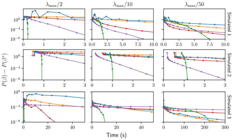
In Figure 6, we present the results of the benchmarks on simulated data. We see that for smaller fractions of $\lambda_{\text{max}}$ our hybrid algorithm allows significant speedup in comparison to its competitors mainly when the number of features is larger than the number of samples. On very large scale data such as in simulated data setting $3$ , we see that the hybrid solver is faster than its competitors by one or two orders of magnitude.

For the second scenario, notice that all solvers take considerably longer than the oracle CD method to reach convergence. This gap is a consequence of Cholesky factorization in the case of ADMM and computation of $\lVert{X}\rVert_{2}$ in the remaining cases. For the hybrid method, we can avoid this cost, with little impact on performance, since $\lVert{X}\rVert_{2}$ is used only in the PGD step.

3.2 Real data

The datasets used for the experiments have been described in Table 3 and were obtained from Chang & Lin 2011; 2; 1.

Table 3: List of real datasets used in our experiments. See Table 4 in Appendix E for references on these datasets.

Dataset	$n$	$p$	Density
bcTCGA	$536$	$17\,322$	$1$
news20	$19\,996$	$1\,355\,191$	$0.000\,335\,7$
rcv1	$20\,242$	$44\,504$	$0.001\,66$
Rhee2006	$842$	$360$	$0.024\,69$

Figure 7 shows the suboptimality for the objective function $P$ as a function of the time for the four different datasets. We see that when the regularization parameter is set at $\lambda_{\text{max}}/2$ and $\lambda_{\text{max}}/10$ , our proposed solver is faster than all its competitors—especially when the datasets become larger. This is even more visible for the news20 dataset where we see that our proposed method is faster by at least one order of magnitude.

When the parametrization value is set to $\lambda_{\text{max}}/50$ , our algorithm remains competitive on the different datasets. It can be seen that the different competitors do not behave consistently across the datasets. For example, the Newt-ALM method is very fast on the bcTCGA dataset but is very slow on the news20 dataset whereas the hybrid method remains very efficient in both settings.

4 DISCUSSION

In this paper we have presented a new, fast algorithm for solving Sorted L-One Penalized Estimation (SLOPE). Our method relies on a combination of proximal gradient descent to identify the cluster structure of the solution and coordinate descent to allow the algorithm to take large steps. In our results, we have shown that our method often outperforms all competitors by orders of magnitude for high-to-medium levels of regularization and typically performs among the best algorithms for low levels of regularization.

We have not, in this paper, considered using screening rules for SLOPE (Larsson et al. 2020; Elvira & Herzet 2021). Although screening rules work for any algorithm considered in this article, they are particularly effective when used in tandem with coordinate descent (Fercoq et al. 2015) and, in addition, easy to implement due to the nature of coordinate descent steps. Coordinate descent is moreover especially well-adapted to fitting a path of $\lambda$ sequences (Friedman et al. 2007; Friedman et al. 2010), which is standard practice during cross-validating to obtain an optimal $\lambda$ sequence.

Future research directions may include investigating alternative strategies to split clusters, for instance by considering the directional derivatives with respect to the coefficients of an entire cluster at once. Another potential approach could be to see if the full proximal gradient steps might be replaced with batch stochastic gradient descent in order to reduce the costs of these steps. It would also be interesting to consider whether gap safe screening rules might be used not only to screen predictors, but also to deduce whether clusters are able to change further during optimization. Finally, combining cluster identification of proximal gradient descent with solvers such as second order ones as in Bareilles et al. 2022 is a direction of interest.

Acknowledgements

The experiments presented in this paper were carried out using the HPC facilities of the University of Luxembourg (Varrette et al. 2022) (see hpc.uni.lu).

The results shown here are in whole or part based upon data generated by the TCGA Research Network: https://www.cancer.gov/tcga.

rangepages34 rangepages20 rangepages1 rangepages38 rangepages122 rangepages22 rangepages-1 rangepages33 rangepages8 rangepages13 rangepages10 rangepages9 rangepages31 rangepages22 rangepages6 rangepages21 rangepages34 rangepages6 rangepages12 rangepages24 rangepages37 rangepages25 rangepages29 rangepages6 rangepages1 rangepages20 rangepages42 rangepages49 rangepages28

References

Bareilles et al. (2022) Gilles Bareilles, Franck Iutzeler and Jérôme Malick “Newton acceleration on manifolds identified by proximal gradient methods” In Mathematical Programming Springer, 2022, pp. 1–34
Beck & Teboulle (2009) Amir Beck and Marc Teboulle “A Fast Iterative Shrinkage-Thresholding Algorithm for Linear Inverse Problems” In SIAM Journal on Imaging Sciences 2.1, 2009, pp. 183–202
Bogdan et al. (2013) Małgorzata Bogdan, Ewout van Berg, Weijie Su and Emmanuel Candès “Statistical Estimation and Testing via the Sorted L1 Norm”, 2013 arXiv:1310.1969 [math, stat]
Bogdan et al. (2022) Małgorzata Bogdan, Xavier Dupuis, Piotr Graczyk, Bartosz Kołodziejek, Tomasz Skalski, Patrick Tardivel and Maciej Wilczyński “Pattern Recovery by SLOPE” arXiv, 2022, pp. 27 DOI: 10.48550/arXiv.2203.12086
Bogdan et al. (2015) Małgorzata Bogdan, Ewout van den Berg, Chiara Sabatti, Weijie Su and Emmanuel Candès “SLOPE - Adaptive Variable Selection via Convex Optimization” In The annals of applied statistics 9.3, 2015, pp. 1103–1140
Boyd et al. (2011) Stephen Boyd, N. Parikh, E. Chu, B. Peleato and J. Eckstein “MATLAB Scripts for Alternating Direction Method of Multipliers”, 2011 Stanford University URL: https://web.stanford.edu/˜boyd/papers/admm/
Boyd et al. (2010) Stephen Boyd, Neil Parikh, Eric Chu, Borja Peleato and Jonathan Eckstein “Distributed Optimization and Statistical Learning via the Alternating Direction Method of Multipliers” In Foundations and Trends® in Machine Learning 3.1, 2010, pp. 1–122
[1] Patrick Breheny “Patrick Breheny” University of Iowa URL: https://myweb.uiowa.edu/pbreheny/
Breheny & Huang (2011) Patrick Breheny and Jian Huang “Coordinate Descent Algorithms for Nonconvex Penalized Regression, with Applications to Biological Feature Selection” In The Annals of Applied Statistics 5.1, 2011, pp. 232–253
Chang & Lin (2011) Chih-Chung Chang and Chih-Jen Lin “LIBSVM: A Library for Support Vector Machines” In ACM Transactions on Intelligent Systems and Technology 2.3, 2011, pp. 27:1–27:27
[2] Chih-Chung Chang and Chih-Jen Lin “LIBSVM Data: Classification, Regression, and Multi-Label” LIBSVM - A library for Support Vector Machines URL: https://www.csie.ntu.edu.tw/˜cjlin/libsvmtools/datasets/
Combettes & Wajs (2005) Patrick Combettes and Valérie Wajs “Signal recovery by proximal forward-backward splitting” In Multiscale modeling & simulation 4.4 SIAM, 2005, pp. 1168–1200
Dupuis & Tardivel (2022) Xavier Dupuis and Patrick Tardivel “Proximal operator for the sorted l1 norm: Application to testing procedures based on SLOPE” In Journal of Statistical Planning and Inference 221, 2022, pp. 1–8
Elvira & Herzet (2021) Clément Elvira and Cédric Herzet “Safe Rules for the Identification of Zeros in the Solutions of the SLOPE Problem” arXiv, 2021 arXiv:2110.11784
Fan & Li (2001) Jianqing Fan and Runze Li “Variable Selection via Nonconcave Penalized Likelihood and Its Oracle Properties” In Journal of the American Statistical Association 96.456, 2001, pp. 1348–1360
Fercoq et al. (2015) Olivier Fercoq, Alexandre Gramfort and Joseph Salmon “Mind the Duality Gap: Safer Rules for the Lasso” In ICML 37, Proceedings of Machine Learning Research, 2015, pp. 333–342
Figueiredo & Nowak (2016) Mario Figueiredo and Robert Nowak “Ordered Weighted L1 Regularized Regression with Strongly Correlated Covariates: Theoretical Aspects” In AISTATS, 2016, pp. 930–938
Friedman et al. (2007) Jerome Friedman, Trevor Hastie, Holger Höfling and Robert Tibshirani “Pathwise Coordinate Optimization” In The Annals of Applied Statistics 1.2, 2007, pp. 302–332
Friedman et al. (2022) Jerome Friedman, Trevor Hastie, Rob Tibshirani, Balasubramanian Narasimhan, Kenneth Tay, Noah Simon, Junyang Qian and James Yang “Glmnet: Lasso and Elastic-Net Regularized Generalized Linear Models”, 2022 URL: https://CRAN.R-project.org/package=glmnet
Friedman et al. (2010) Jerome Friedman, Trevor Hastie and Robert Tibshirani “Regularization Paths for Generalized Linear Models via Coordinate Descent” In Journal of Statistical Software 33.1, 2010, pp. 1–22
Harris et al. (2020) Charles Harris, K Millman, Stéfan Van, Ralf Gommers, Pauli Virtanen, David Cournapeau, Eric Wieser, Julian Taylor, Sebastian Berg and Nathaniel Smith “Array programming with NumPy” In Nature 585.7825 Nature Publishing Group, 2020, pp. 357–362
Keerthi & DeCoste (2005) S. Keerthi and Dennis DeCoste “A Modified Finite Newton Method for Fast Solution of Large Scale Linear SVMs” In JMLR 6.12, 2005, pp. 341–361
Kos & Bogdan (2020) Michał Kos and Małgorzata Bogdan “On the Asymptotic Properties of SLOPE” In Sankhya A 82.2, 2020, pp. 499–532
Lam et al. (2015) Siu Lam, Antoine Pitrou and Stanley Seibert “Numba: A llvm-based python jit compiler” In Proceedings of the Second Workshop on the LLVM Compiler Infrastructure in HPC, 2015, pp. 1–6
Larsson et al. (2020) Johan Larsson, Małgorzata Bogdan and Jonas Wallin “The Strong Screening Rule for SLOPE” In NeurIPS 33, 2020, pp. 14592–14603
Larsson et al. (2022) Johan Larsson et al. “SLOPE: Sorted L1 Penalized Estimation”, 2022 URL: https://CRAN.R-project.org/package=SLOPE
Lewis (2002) A.. Lewis “Active Sets, Nonsmoothness, and Sensitivity” In SIAM Journal on Optimization 13.3, 2002, pp. 702–725 DOI: 10.1137/S1052623401387623
Lewis et al. (2004) David. Lewis, Yiming Yang, Tony. Rose and Fan Li “RCV1: A New Benchmark Collection for Text Categorization Research” In JMLR 5, 2004, pp. 361–397
Liang et al. (2014) Jingwei Liang, Jalal Fadili and Gabriel Peyré “Local linear convergence of Forward–Backward under partial smoothness” In Advances in neural information processing systems 27, 2014
Luo et al. (2019) Ziyan Luo, Defeng Sun, Kim-Chuan Toh and Naihua Xiu “Solving the OSCAR and SLOPE Models Using a Semismooth Newton-Based Augmented Lagrangian Method” In Journal of Machine Learning Research 20.106, 2019, pp. 1–25
Moreau et al. (2022) Thomas Moreau et al. “Benchopt: Reproducible, efficient and collaborative optimization benchmarks” In NeurIPS, 2022
[3] National Cancer Institute “The Cancer Genome Atlas Program” National Cancer Institute URL: https://www.cancer.gov/about-nci/organization/ccg/research/structural-genomics/tcga
Paige & Saunders (1982) Christopher. Paige and Michael. Saunders “LSQR: An Algorithm for Sparse Linear Equations and Sparse Least Squares” In ACM Transactions on Mathematical Software 8.1, 1982, pp. 43–71
Rhee et al. (2006) Soo-Yon Rhee, Jonathan Taylor, Gauhar Wadhera, Asa Ben-Hur, Douglas. Brutlag and Robert. Shafer “Genotypic Predictors of Human Immunodeficiency Virus Type 1 Drug Resistance” In Proceedings of the National Academy of Sciences 103.46 Proceedings of the National Academy of Sciences, 2006, pp. 17355–17360
Schneider & Tardivel (2020) Ulrike Schneider and Patrick Tardivel “The Geometry of Uniqueness, Sparsity and Clustering in Penalized Estimation” arXiv, 2020, pp. 34 arXiv: http://arxiv.org/abs/2004.09106
Tseng (2001) Paul Tseng “Convergence of a block coordinate descent method for nondifferentiable minimization” In Journal of optimization theory and applications 109.3 Springer, 2001, pp. 475–494
Vaiter et al. (2017) Samuel Vaiter, Charles Deledalle, Jalal Fadili, Gabriel Peyré and Charles Dossal “The Degrees of Freedom of Partly Smooth Regularizers” In Annals of the Institute of Statistical Mathematics 69.4 Springer Nature, 2017, pp. 791–832 DOI: 10.1007/s10463-016-0563-z
Varrette et al. (2022) S. Varrette, H. Cartiaux, S. Peter, E. Kieffer, T. Valette and A. Olloh “Management of an Academic HPC & Research Computing Facility: The ULHPC Experience 2.0” In Proc. of the 6th ACM High Performance Computing and Cluster Technologies Conf. (HPCCT 2022) Fuzhou, China: Association for Computing Machinery (ACM), 2022
Zangwill (1969) Willard. Zangwill “Nonlinear Programming: A Unified Approach” New Orleans, USA: Prentice-Hall, 1969
Zeng & Figueiredo (2014) Xiangrong Zeng and Mario Figueiredo “The Ordered Weighted $\ell_{1}$ Norm: Atomic Formulation, Projections, and Algorithms” arXiv, 2014 arXiv:1409.4271
Zhang (2010) Cun-Hui Zhang “Nearly Unbiased Variable Selection under Minimax Concave Penalty” In The Annals of Statistics 38.2, 2010, pp. 894–942
Zhang et al. (2020) Junzi Zhang, Brendan O’Donoghue and Stephen Boyd “Globally convergent type-I Anderson acceleration for nonsmooth fixed-point iterations” In SIAM Journal on Optimization 30.4 SIAM, 2020, pp. 3170–3197

Supplement to Coordinate Descent for SLOPE

Appendix A PROOFS

A.1 Proof of Theorem 2.2

Let $c^{\setminus k}$ be the set containing all elements of $c$ except the $k$ -th one: $c^{\setminus k}=\{c_{1},\ldots c_{k-1},c_{k+1},\ldots,c_{m}\}$ .

From the observations in Remark 2.1, we have the following cases to consider: $|z|\in c^{\setminus k}$ , $|z|=0$ , and $|z|\notin\{0\}\cup c^{\setminus k}$ .

Since $C(z+\delta h)=C(z)=\mathcal{C}_{k}$ and $\sign(z+\delta h)=\sign(z)$ for $h$ small enough,

$\displaystyle H(z+\delta h)-H(z)$	$\displaystyle=\sum_{j=1}^{p}\|\beta(z+\delta h)_{j}\|\lambda_{(j)^{-}_{z+\delta h}}-\sum_{j=1}^{p}\|\beta(z)_{j}\|\lambda_{(j)^{-}_{z}}$
	$\displaystyle=\sum_{j=1}^{p}(\|\beta(z+\delta h)_{j}\|-\|\beta(z)_{j}\|)\lambda_{(j)^{-}_{z}}$
	$\displaystyle=\sum_{j=1}^{p}(\|\beta(z+\delta h)_{j}\|-\|\beta(z)_{j}\|)\lambda_{(j)^{-}_{z}}$
	$\displaystyle=\sum_{j\in C(z)}^{p}(\|\beta(z+\delta h)_{j}\|-\|\beta(z)_{j}\|)\lambda_{(j)^{-}_{z}}$
	$\displaystyle=\sum_{j\in C(z)}\sign(\beta(z)_{j})(z+\delta h-z)\lambda_{(j)^{-}_{z}}$
	$\displaystyle=\sum_{j\in C(z)}\sign(z)\delta h\lambda_{(j)^{-}_{z}}$
	$\displaystyle=\sum_{j\in\mathcal{C}_{k}}\sign(z)\delta h\lambda_{(j)^{-}_{z}}\,.$	(11)

Case 2

Then if $z\neq 0$ and $|z|$ is equal to one of the $c_{i}$ ’s, $i\neq k$ , one has $C(z)=\mathcal{C}_{k}\cup\mathcal{C}_{i}$ , $C(z+\delta h)=\mathcal{C}_{k}$ , and $\sign(z+\delta h)=\sign(z)$ for $h$ small enough. Thus

$\displaystyle H(z+\delta h)-H(z)$	$\displaystyle=\sum_{j=1}^{p}\|\beta(z+\delta h)_{j}\|\lambda_{(j)^{-}_{z+\delta h}}-\sum_{i=1}^{p}\|\beta(z)_{j}\|\lambda_{(j)^{-}_{z}}$
	$\displaystyle=\sum_{j\in\mathcal{C}_{k}\cup\mathcal{C}_{i}}\left(\|\beta(z+\delta h)_{j}\|\lambda_{(j)^{-}_{z+\delta h}}-\|\beta(z)_{j}\|\lambda_{(j)^{-}_{z}}\right)$
	$\displaystyle=\sum_{j\in\mathcal{C}_{k}}\left(c_{i}+\delta h\right)\lambda_{(i)^{-}_{z+\delta h}}-c_{i}\lambda_{(i)^{-}_{z}}+\sum_{j\in\mathcal{C}_{i}}\left(c_{i}\lambda_{(j)^{-}_{z+\delta h}}-c_{i}\lambda_{(i)^{-}_{z}}\right)\,.$	(12)

Note that there is an ambiguity in terms of permutation, since, due to the clustering, there can be more than one permutation reordering $\beta(z)$ . However, choosing any such permutation result in the same values for the computed sums.

Case 3

Finally let us treat the case $z=0$ . If $c_{m}=0$ then the proof proceeds as in case 2, with the exception that $|\beta(z+\delta h)|=h$ and so the result is just:

\displaystyle H(z+\delta h)-H(z)

\displaystyle=h\sum_{j\in\mathcal{C}_{k}}\lambda_{(i)^{-}_{z+\delta h}}\,.

(13)

If $c_{m}\neq 0$ , then the computation proceeds exactly as in case 1.

A.2 Proof of Theorem 2.3

Recall that $G(z):\mathbb{R}\to\mathbb{R}$ is a convex, continuous piecewise-differentiable function with breakpoints whenever $|z|=c_{i}^{\setminus k}$ or $z=0$ . Let $\gamma=c_{k}\lVert{\tilde{x}}\rVert^{2}+\tilde{x}^{T}r$ and $\omega=\lVert{\tilde{x}}\rVert^{2}$ and note that the optimality criterion for ((6)) is

\delta(\omega z-\gamma)+H^{\prime}(z;\delta)\geq 0,\quad\forall\delta\in\{-1,1\},

which is equivalent to

\omega z-H^{\prime}(z;-1)\leq\gamma\leq\omega z+H^{\prime}(z;1).

(14)

We now proceed to show that there is a solution $z^{*}\in\argmin_{z\in\mathbb{R}}H(z)$ for every interval over $\gamma\in\mathbb{R}$ .

First, assume that the first case in the definition of $T$ holds and note that this is equivalent to (14) with $z=0$ since $C({\varepsilon_{c}})=C(-{\varepsilon_{c}})$ and $\lambda_{(j)^{-}_{-{\varepsilon_{c}}}}=\lambda_{(j)^{-}_{{\varepsilon_{c}}}}$ . This is sufficient for $z^{*}=0$ .

Next, assume that the second case holds and observe that this is equivalent to (14) with $z=c_{i}^{\setminus k}$ , since $C(c_{i}+{\varepsilon_{c}})=C(-c_{i}-{\varepsilon_{c}})$ and $C(-c_{i}+{\varepsilon_{c}})=C(c_{i}-{\varepsilon_{c}})$ . Thus $z^{*}=\sign(\gamma)c_{i}^{\setminus k}$ .

For the third case, we have

\sum_{j\in C(c_{i}+{\varepsilon_{c}})}\lambda_{(j)^{-}_{c_{i}+{\varepsilon_{c}}}}=\sum_{j\in C(c_{i-1}-{\varepsilon_{c}})}\lambda_{(j)^{-}_{c_{i-1}-{\varepsilon_{c}}}}

and therefore (14) is equivalent to

c_{i}<\frac{1}{\omega}\bigg(|\gamma|-\sum_{j\in C(c_{i}+{\varepsilon_{c}})}\lambda_{(j)^{-}_{c_{i}+{\varepsilon_{c}}}}\bigg)<c_{i-1}.

Now let

z^{*}=\frac{\sign(\gamma)}{\omega}\bigg(|\gamma|-\sum_{j\in C(c_{i}+{\varepsilon_{c}})}\lambda_{(j)^{-}_{c_{i}+{\varepsilon_{c}}}}\bigg)

(15)

and note that $|z^{*}|\in\big(c_{i}^{\setminus k},c_{i-1}^{\setminus k}\big)$ and hence

\frac{1}{\omega}\bigg(|\gamma|-\sum_{j\in C(c_{i}+{\varepsilon_{c}})}\lambda_{(j)^{-}_{c_{i}+{\varepsilon_{c}}}}\bigg)=\frac{1}{\omega}\bigg(|\gamma|-\sum_{j\in C(z^{*})}\lambda_{(j)^{-}_{z^{*}}}\bigg).

Furthermore, since $G$ is differentiable in $\big(c_{i}^{\setminus k},c_{i-1}^{\setminus k}\big)$ , we have

\frac{\partial}{\partial z}G(z)\Big|_{z=z^{*}}=\omega z^{*}-\gamma+\sign(z^{*})\sum_{j\in C(z^{*})}\lambda_{(j)^{-}_{z^{*}}}=0,

and therefore (15) must be the solution.

The solution for the last case follows using reasoning analogous to that of the third case.

A.3 Proof of Lemma 2.6

To prove the lemma, we will show that $\lim_{t\rightarrow\infty}\beta^{(t)}\in\Omega=\{\beta:0\in\partial P(\beta)\}$ using Convergence Theorem A in Zangwill 1969. For simplicity, we assume that the point to set map $A$ is generated by $v$ iterations of Algorithm 1, that is $A(\beta^{(0)})=\{\beta^{(vi)}\}_{i=0}^{\infty}$ . To be able to use the theorem, we need the following assumptions to hold.

1.

The set of iterates, $A(\beta^{(0)})$ is in a compact set.
2.

$P$ is continuous and if $\beta\notin\Omega=\{\beta:0\in\partial P(\beta)\}$ , then for any $\hat{\beta}\in A(\beta)$ it holds that $P(\hat{\beta})<P(\beta)$ .
3.

If $\beta\in\Omega=\{\beta:0\in\partial P(\beta)\}$ , then for any $\hat{\beta}\in A(\beta)$ it holds that $P(\hat{\beta})\leq P(\beta)$ .

Before tackling these three assumptions, we decompose the map into two parts: $v-1$ coordinate descent steps, $T_{\text{CD}}$ , and one proximal gradient decent step, $T_{\text{PGD}}$ . This clearly means that

P(T_{\text{CD}}(\beta))\leq P(\beta)

for all $\beta\in\mathbb{R}^{p}$ . For $T_{\text{PGD}}$ , we have two useful properties: first, if $||T_{\text{PGD}}(\beta)-\beta||=0$ , then by Lemma 2.2 in Beck & Teboulle 2009 it follows that $\beta\in\Omega$ . Second, by Lemma 2.3 in Beck & Teboulle 2009, using $x=y$ , it follows that

P(T_{\text{PGD}}(\beta))-P(\beta)\leq-\frac{L(f)}{2}||T_{\text{PGD}}(\beta)-\beta||^{2},

where $L(f)$ is the Lipschitz constant of the gradient of $f(\beta)=\frac{1}{2}||y-X\beta||^{2}$ .

We are now ready to prove that the three assumptions hold.

•

Assumption 1 follows from the fact that the level sets of $P$ are compact and from $P(T_{PGD}(\beta))\leq P(\beta)$ and $P(T_{CD}(\beta))\leq P(\beta)$ .
•

Assumption 2 holds since if $\beta\notin\Omega$ , it follows that $||T_{\text{PGD}}(\beta)-\beta||>0$ and thus $P(T_{\text{PGD}}(\beta))<P(\beta)$ .
•

Assumption 3 follows from $P(T_{PGD}(\beta))\leq P(\beta)$ and $P(T_{CD}(\beta))\leq P(\beta)$ .

Using Theorem 1 from Zangwill 1969, this means that Algorithm 1 converges as stated in the lemma.

A.4 Partial Smoothness of the Sorted $\ell_{1}$ Norm

In this section, we prove that the sorted $\ell_{1}$ norm $J$ is partly smooth (Lewis 2002). This allows us to apply results about the structure identification of the proximal gradient algorithm.

Definition A.1.

Let $J$ be a proper closed convex function and $x$ a point of its domain such that $\partial J(x)\neq\emptyset$ . $J$ is said to be partly smooth at $x$ relative to a set $\mathcal{M}$ containing $x$ if:

1.

$\mathcal{M}$ is a $C^{2}$ -manifold around $x$ and $J$ restricted to $\mathcal{M}$ is $C^{2}$ around $x$ .
2.

The tangent space of $\mathcal{M}$ at $x$ is the orthogonal of the parallel space of $\partial J(x)$ .
3.

$\partial J$ is continuous at $x$ relative to $\mathcal{M}$ .

Because the sorted $\ell_{1}$ norm is a polyhedral, it follows immediately that it is partly smooth (Vaiter et al. 2017, Example 18). But since we believe a direct proof is interesting in and of itself, we provide and prove the following proposition here.

Proposition A.2.

Suppose that the regularization parameter $\lambda$ is a strictly decreasing sequence. Then the sorted $\ell_{1}$ norm is partly smooth at any point of $\mathbb{R}^{p}$ .

Proof.

Let $m$ be the number of clusters of $x$ and $\mathcal{C}_{1},\ldots,\mathcal{C}_{m}$ be those clusters, and let $c_{1}>\cdots>c_{m}>0$ be the value of $\lvert x\rvert$ on the clusters.

We define $\varepsilon_{c}$ as in Equation 9 and let $\mathcal{B}=\{u\in\mathbb{R}^{p}:\lVert u-x\rVert_{\infty}<\varepsilon_{c}/2\}$ . Let $v_{k}\in\mathbb{R}^{p}$ for $k\in[m]$ be equal to $\sign(x_{\mathcal{C}_{k}})$ on $\mathcal{C}_{k}$ and to 0 outside, such that $x=\sum_{k=1}^{m}c_{k}v_{k}$ . We define

\mathcal{M}=\begin{cases}\Span(v_{1},\ldots,v_{m})\cap\mathcal{B}\,&\text{if }c_{m}\neq 0\,,\\ \Span(v_{1},\ldots,v_{m-1})\cap\mathcal{B}\,&\text{otherwise}\,.\end{cases}

We will show that $J$ is partly smooth at $x$ relative to $\mathcal{M}$ .

As a first statement, we prove that any $u\in\mathcal{M}$ shares the same clusters as $x$ . For any $u\in\mathcal{M}$ there exists $c^{\prime}\in\mathbb{R}^{m}$ , $u=\sum_{k=1}^{m}c^{\prime}_{k}v_{k}$ (with $c^{\prime}_{m}=0$ if $c_{m}=0$ ). Suppose that there exist $k\neq k^{\prime}$ such that $c^{\prime}_{k}=c^{\prime}_{k^{\prime}}$ . Then since $\lVert x-u\rVert_{\infty}=\max_{k}|c_{k}-c^{\prime}_{k}|$ and $|c_{k}-c_{k^{\prime}}|>\varepsilon_{c}$ , one has:

	$\displaystyle\varepsilon_{c}<\|c_{k}-c_{k^{\prime}}\|$	$\displaystyle=\|c_{k}-c^{\prime}_{k}+c^{\prime}_{k^{\prime}}-c_{k^{\prime}}\|$
		$\displaystyle\leq\|c_{k}-c^{\prime}_{k}\|+\|c^{\prime}_{k^{\prime}}-c_{k^{\prime}}\|$
		$\displaystyle\leq 2\lVert x-u\rVert_{\infty}$
		$\displaystyle\leq\varepsilon_{c}\,.$

This shows that clusters of any $u\in\mathcal{M}$ are equal to clusters of $x$ . Further, clearly the tangent space of $\mathcal{M}$ at $x$ is $\Span(v_{1},\ldots,v_{m})$ if $c_{m}\neq 0$ and $\Span(v_{1},\ldots,v_{m-1})$ otherwise.

1.

The set $\mathcal{M}$ is then the intersection of a linear subspace and an open ball, and hence is a $\mathcal{C}^{2}$ manifold. Since the clusters of any $u\in\mathcal{M}$ are the same as the clusters of $x$ , we can write that

$\displaystyle{}J(u)=\sum_{k=1}^{m}\left(\sum_{j\in\mathcal{C}_{k}}\lambda_{j}\right)c_{k}^{\prime}\kern 5.0pt,$ (16)

and hence $J$ is linear on $\mathcal{M}$ and thus $\mathcal{C}^{2}$ around $x$ .

We let $x_{\downarrow}$ denote a version of $x$ sorted in non-increasing order and let $R:\mathbb{R}^{p}\rightarrow\mathbb{N}^{p}$ be the function that returns the ranks of the absolute values of its argument. The subdifferential of $J$ at $x$ (Larsson et al. 2020, Thm. 1)⁶⁶ 6 We believe there to be a typo in the definition of the subgradient in (Larsson et al. 2020, Thm. 1). We believe the argument of $R$ should be $g$ , not $s$ , since otherwise there is a dimension mismatch. is the set of all $g\in\mathbb{R}^{p}$ such that

\displaystyle g_{\mathcal{C}_{i}}\in\mathcal{G}_{i}\triangleq\left\{s\in\mathbb{R}^{|C_{i}|}:\begin{cases}\cumsum(|s|_{\downarrow}-\lambda_{R(g)_{\mathcal{C}_{i}}})\preceq 0&\text{if }x_{\mathcal{C}_{i}}=\textbf{0}\,,\\ \cumsum(|s|_{\downarrow}-\lambda_{R(g)_{\mathcal{C}_{i}}})\preceq 0\\ \quad\text{ and }\sum_{j\in\mathcal{C}_{i}}(|s_{j}|-\lambda_{R(g)_{\mathcal{C}_{i}}})=0\\ \quad\text{ and }\sign(x_{\mathcal{C}_{i}})=\sign(s)&\mathrm{otherwise.}\end{cases}\right\}

(17)

Hence, the problem can be decomposed over clusters. We will restrict the analysis to a single $\mathcal{C}_{i}$ without loss of generality and proceed in $\mathbb{R}^{|\mathcal{C}_{i}|}$ .

•

First we treat the case where $|\mathcal{C}_{i}|=1$ and $x_{\mathcal{C}_{i}}\neq 0$ . The set $\mathcal{G}_{i}$ is then the singleton $\{\sign(x_{\mathcal{C}_{i}})\lambda_{R(s)_{\mathcal{C}_{i}}}\}$ and its parallel space is simply $\{0\}$ . Hence, $\parset(\mathcal{G}_{i})^{\perp}=\mathbb{R}=\Span(\sign(x)_{\mathcal{C}_{i}})$ .
•

Then, we study the case where $|\mathcal{C}_{i}|\neq 1$ and $x_{\mathcal{C}_{i}}\neq\textbf{0}$ . Since for all $j\in[p]$ , $\lambda_{j}\neq 0$ and $\lambda$ is a strictly decreasing sequence, we have that for $\varepsilon>0$ small enough, the $|\mathcal{C}_{i}|-1$ points $\lambda_{R(g)_{\mathcal{C}_{i}}}+\varepsilon[-\sign(x_{\mathcal{C}_{i}})_{1},\sign(x_{\mathcal{C}_{i}})_{2},0,\ldots,0]^{T}$ , $\lambda_{R(g)_{\mathcal{C}_{i}}}+\varepsilon[0,-\sign(x_{\mathcal{C}_{i}})_{2},\sign(x_{\mathcal{C}_{i}})_{3},\ldots,0]^{T}$ , $\ldots$ , $\lambda_{R(g)_{\mathcal{C}_{i}}}+\varepsilon[0,0,0,\ldots,-\sign(x_{\mathcal{C}_{i}})_{|\mathcal{C}_{i}|-1},\sign(x_{\mathcal{C}_{i}})_{|\mathcal{C}_{i}|}]^{T}$ belong to $\mathcal{G}_{i}$ . Since these vectors are linearly independent, and using the last equality in the feasible set that, we have that

$\displaystyle\sum_{j\in\mathcal{C}_{i}}\sign(x_{j})s_{j}=\sum_{j\in\mathcal{C}_{i}}\lambda_{R(g)_{\mathcal{C}_{i}}}\kern 5.0pt.$

Its parallel space is simply the set $\{s\in\mathbb{R}^{|\mathcal{C}_{i}|}:\sum_{j\in\mathcal{C}_{i}}\sign(x_{j})s_{j}=0\}$ , that is just $\Span(\sign(x_{\mathcal{C}_{i}}))^{\perp}$ . Hence $\parset(\mathcal{G}_{i})^{\perp}=\Span(\sign(x_{\mathcal{C}_{i}}))$ .
•

Finally, we study the case where $x_{\mathcal{C}_{m}}=\textbf{0}$ . Then the $\ell_{\infty}$ ball $\{s\in\mathbb{R}^{|\mathcal{C}_{m}|}:\|s\|_{\infty}\leq\lambda_{p}\}$ is contained in the feasible set of the differential, hence the parallel space of $\mathcal{G}_{m}$ is $\mathbb{R}^{|\mathcal{C}_{m}|}$ and its orthogonal is reduced to $\{\mathbf{0}\}$ .

We can now prove that $\parset(\partial J(x))^{\perp}$ is the tangent space of $\mathcal{M}$ . From the decomposability of $\partial J$ (Equation 17), one has that $u\in\parset(\partial J(x))^{\perp}$ if and only if $u_{\mathcal{C}_{i}}\in\parset(\mathcal{G}_{i})^{\perp}$ for all $i\in[m]$ .

If $c_{m}>0$ , we have

$\displaystyle\parset(\partial J(x))^{\perp}$	$\displaystyle=\{u\in\mathbb{R}^{p}:\forall i\in[m],u_{\mathcal{C}_{i}}\in\parset(\mathcal{G}_{i})^{\perp}\}$	(18)
	$\displaystyle=\{u\in\mathbb{R}^{p}:\forall i\in[m],u_{\mathcal{C}_{i}}\in\Span(\sign(x_{\mathcal{C}_{i}}))\}$
	$\displaystyle=\Span(v_{1},\ldots,v_{m})\,.$

If $c_{m}=0$ , we have

$\displaystyle\parset(\partial J(x))^{\perp}$	$\displaystyle=\{u\in\mathbb{R}^{p}:\forall i\in[m],u_{\mathcal{C}_{i}}\in\parset(\mathcal{G}_{i})^{\perp}\}$	(19)
	$\displaystyle=\{u\in\mathbb{R}^{p}:\forall i\in[m-1],u_{\mathcal{C}_{i}}\in\Span(\sign(x_{\mathcal{C}_{i}}))\quad\&\quad u_{\mathcal{C}_{m}}=\mathbf{0}\}$
	$\displaystyle=\Span(v_{1},\ldots,v_{m-1})\,.$

3.

The subdifferential of $J$ is a constant set locally around $x$ along $\mathcal{M}$ since the clusters of any point in the neighborhood of $x$ in $\mathcal{M}$ shares the same clusters with $x$ . This shows that it is continuous at $x$ relative to $\mathcal{M}$ .

∎

Remark A.3.

We believe that the assumption $\lambda_{1}>\cdots>\lambda_{p}$ can be lifted, since for example the $\ell_{1}$ and $\ell_{\infty}$ norms are particular instances of $J$ that violate this assumption, yet are still partly smooth. Hence this assumption could probably be lifted in a future work using a slightly different proof.

Appendix B ADDITIONAL EXPERIMENTS

B.1 glmnet versus SLOPE Comparison

In this experiment, we ran the glmnet (Friedman et al. 2022) and SLOPE (Larsson et al. 2022) packages on the bcTCGA dataset, selecting the regularization sequence $\lambda$ such that there were 100 nonzero coefficients and clusters at the optimum for glmnet and SLOPE respectively. We used a duality gap of $10^{-6}$ as stopping criteria. The features were centered by their means and scaled by their standard deviation. The code is available at github.com/jolars/slopecd.

B.2 Study on Proximal Gradient Descent Frequency

To study the impact of the frequence at which the PGD step in the hybrid solver is used, we performed a comparative study with the rcv1 dataset. We set this parameter to values ranging from $1$ i.e., the PGD algorithm, to 9 meaning that a PGD step is taken every $9$ epochs. The sequence of $\lambda$ has been set with the Benjamini-Hochberg method and parametrized with $0.1\lambda_{\text{max}}$ .

Figure 8 shows the suboptimality score as a function of the time for the different values of the parameter controlling the frequency at which a PGD step is going to be taken. A first observation is that as long as this parameter is greater than $1$ meaning that we perform some coordinate descent steps, we observe a significant speed-up. For all our experiments, this parameter was set to $5$ . The figure also shows that any choice between $3$ and $9$ would lead to similar performance for this example.

Figure 8: Suboptimality score as a function of the time for different frequencies of the PDG step inside the hybrid solver for the rcv1 dataset

B.3 Benchmark with Different Parameters for the ADMM Solver

We reproduced the benchmarks setting described in Section 3 for the simulated and real data. We compared the ADMM solver with our hybrid algorithm for different values of the augmented Lagrangian parameter $\rho$ . We tested three different values $10,100$ and $1000$ as well as the adaptive method (Boyd et al. 2010, Sec. 3.4.1).

We present in Figure 9 and Figure 10 the suboptimality score as a function the time for the different solvers. We see that the best value for $\rho$ depends on the dataset and the regularization strengh. The value chosen for the main benchmark (Section 3) performs well in comparison to other ADMM solvers. Nevertheless, our hybrid approach is consistently faster than the different ADMM solvers.

Appendix C EXTENSIONS TO OTHER DATAFITS

Our algorithm straightforwardly generalizes to problems where the quadratic datafit $\frac{1}{2}\lVert y-X\beta\rVert^{2}$ is replaced by $F(\beta)=\sum_{i=1}^{n}f_{i}(X_{i:}^{\top}\beta)$ , where the $f_{i}$ ’s are $L$ smooth (and so $F$ is $L*\lVert X\rVert_{2}^{2}$ -smooth), such as logistic regression.

In that case, one has by the descent lemma applied to $F(\beta(z))$ , using $F(\beta)=F(\beta(c_{k}))$ ,

F(\beta(z))+H(z)\leq F(\beta)+\sum_{j\in\mathcal{C}_{k}}\nabla_{j}F(\beta)\sign\beta_{j}(z-c_{k})+\frac{L\lVert\tilde{x}\rVert^{2}}{2}(z-c_{k})^{2}+H(z)

(20)

and so a majorization-minimization approach can be used, by minimizing the right-hand side instead of directly minimizing $F(\beta(z))+H(z)$ . Minimizing the RHS, up to rearranging, is of the form of (6).

Appendix D IMPLEMENTATION DETAILS OF SOLVERS

D.1 ADMM

Our implementation of the solver is based on Boyd et al. 2011. For high-dimensional sparse $X$ , we use the numerical LSQR algorithm (Paige & Saunders 1982) instead of the typical direct linear system solver. We originally implemented the solver using the adaptive step size ( $\rho$ ) scheme from Boyd et al. 2010 but discovered that it performed poorly. Instead, we used $\rho=100$ and have provided benchmarks of the alternative configurations in Section B.3.

D.2 Newt-ALM

The implementation of the solver is based on the pseudo-code provided in Luo et al. 2019. According to the authors’ suggestions, we use the Matrix inversion lemma for high-dimensional and sparse $X$ and the preconditioned conjugate gradient method if, in addition, $n$ is large. Please see the source code for further details regarding hyper-parameter choices for the algorithm.

After having completed our own implementation of the algorithm, we received an implementation directly from the authors. Since our own implementation performed better, however, we opted to use it instead.

Appendix E REFERENCES AND SOURCES FOR DATASETS

In Table 4, we list the reference and source (from which the data was gathered) for each of the real datasets used in our experiments.

Table 4: Sources and references for the real data sets used in our experiments.

Dataset	Reference	Source
bcTCGA	3	1
news20	Keerthi & DeCoste 2005	2
rcv1	Lewis et al. 2004	2
Rhee2006	Rhee et al. 2006	1

	$\displaystyle\varepsilon_{c}<\|c_{k}-c_{k^{\prime}}\|$	$\displaystyle=\|c_{k}-c^{\prime}_{k}+c^{\prime}_{k^{\prime}}-c_{k^{\prime}}\|$
		$\displaystyle\leq\|c_{k}-c^{\prime}_{k}\|+\|c^{\prime}_{k^{\prime}}-c_{k^{\prime}}\|$
		$\displaystyle\leq 2\lVert x-u\rVert_{\infty}$
		$\displaystyle\leq\varepsilon_{c}\,.$