Maximum Likelihood Learning of Unnormalized Models
for Simulation-Based Inference
Abstract
We introduce two synthetic likelihood methods for Simulation-Based Inference (SBI), to conduct either amortized or targeted inference from experimental observations when a high-fidelity simulator is available. Both methods learn a conditional energy-based model (EBM) of the likelihood using synthetic data generated by the simulator, conditioned on parameters drawn from a proposal distribution. The learned likelihood can then be combined with any prior to obtain a posterior estimate, from which samples can be drawn using MCMC. Our methods uniquely combine a flexible Energy-Based Model and the minimization of a KL loss: this is in contrast to other synthetic likelihood methods, which either rely on normalizing flows, or minimize score-based objectives; choices that come with known pitfalls. We demonstrate the properties of both methods on a range of synthetic datasets, and apply them to a neuroscience model of the pyloric network in the crab, where our method outperforms prior art for a fraction of the simulation budget.
Keywords:
Machine Learning, ICML1 Introduction
Simulation-based modeling expresses a system as a probabilistic program (Ghahramani 2015), which describes, in a mechanistic manner, how samples from the system are drawn given the parameters of the said system. This probabilistic program can be concretely implemented in a computer - as a simulator - from which synthetic parameter-samples pairs can be drawn. This setting is common in many scientific and engineering disciplines such as stellar events in cosmology (Alsing et al. 2018; Schafer & Freeman 2012), particle collisions in a particle accelerator for high energy physics (Eberl 2003; Sjöstrand et al. 2008), and biological neural networks in neuroscience (Markram et al. 2015; Pospischil et al. 2008). Describing such systems using a probabilistic program often turns out to be easier than specifying the underlying probabilistic model with a tractable probability distribution. We consider the task of inference for such systems, which consists in computing the posterior distribution of the parameters given observed (non-synthetic) data. When a likelihood function of the simulator is available alongside with a prior belief on the parameters, inferring the posterior distribution of the parameters given data is possible using Bayes’ rule. Traditional inference methods such as variational techniques (Wainwright & Jordan 2008) or Markov Chain Monte Carlo (Andrieu et al. 2003) can then be used to produce approximate posterior samples of the parameters that are likely to have generated the observed data. Unfortunately, the likelihood function of a simulator is computationally intractable in general, thus making the direct application of traditional inference techniques unusable for simulation-based modelling.
Simulation-Based Inference (SBI) methods (Cranmer et al. 2020) are methods specifically designed to perform inference in the setting of a simulator with an intractable likelihood. These methods repeatedly generate synthetic data using the simulator to build an estimate of the posterior, that either can be used for any observed data (resulting in a so-called amortized inference procedure) or one that is targeted for a specific observation. While the accuracy of inference increases as more simulations are run, so does computational cost, especially when the simulator is expensive, which is common in many physics applications (Cranmer et al. 2020). In high-dimensional settings, early simulation-based inference techniques such as Approximate Bayesian Computation (ABC) (Marin et al. 2012) struggle to generate high quality posterior samples at a reasonable cost, since ABC repeatedly rejects simulations that fail to reproduce the observed data (Beaumont et al. 2002). More recently, model-based inference methods (Wood 2010; Papamakarios et al. 2019; Hermans et al. 2020; Greenberg et al. 2019), which encode information about the simulator via a parametric density (-ratio) estimator of the data, have been shown to drastically reduce the number of simulations needed to reach a given inference precision (Lueckmann et al. 2021). The computational gains are particularly important when comparing ABC to targeted SBI methods, implemented in a multi-round procedure that refines the model around the observed data, by sequentially simulating data points that are closer to the observed ones (Greenberg et al. 2019; Papamakarios et al. 2019; Hermans et al. 2020).
Previous model-based SBI methods have used their parametric estimator to learn the likelihood (e.g. the conditional density specifying the probability of an observation being simulated given a specific parameter set, Wood 2010; Papamakarios et al. 2019; Pacchiardi & Dutta 2022), the likelihood-to-marginal ratio (Hermans et al. 2020), or the posterior function directly (Greenberg et al. 2019). We focus in this paper on likelihood-based (also called Synthetic Likelihood; SL, in short) methods, of which two main instances exist: (Sequential) Neural Likelihood Estimation (or (S)NLE) (Papamakarios et al. 2019), which learns a likelihood estimate using a normalizing flow trained by optimizing a Maximum Likelihood (ML) loss; and Score Matched Neural Likelihood Estimation (SMNLE Pacchiardi & Dutta 2022), which learns an unnormalized (or Energy-Based, LeCun et al. 2006) likelihood model trained using conditional score matching. Recently, SNLE was applied successfully to challenging neural data (Deistler et al. 2021). However, limitations still remain in the approaches taken by both (S)NLE and SMNLE. On the one hand, flow-based models may need to use very complex architectures to properly approximate distributions with rich structure such as multi-modality (Kong & Chaudhuri 2020; Cornish et al. 2020). On the other hand, score matching, the objective of SMNLE, minimizes the Fisher Divergence between the data and the model, a divergence that fails to capture important features of probability distributions such as mode proportions (Wenliang & Kanagawa 2020; Zhang et al. 2022). This is unlike Maximimum-Likelihood based-objectives, whose maximizers satisfy attractive theoretical properties (Bickel & Doksum 2015).
Contributions. In this work, we introduce Amortized Unnormalized Likelihood Neural Estimation (AUNLE), and Sequential UNLE, a pair of SBI Synthetic Likelihood methods performing respectively sequential and targeted inference. Both methods learn a Conditional Energy Based Model of the simulator’s likelihood using a Maximum Likelihood (ML) objective, and perform MCMC on the posterior estimate obtained after invoking Bayes’ Rule. While posteriors arising from conditional EBMs exhibit a particular form of intractability called double intractability, which requires the use of tailored MCMC techniques for inference, we train AUNLE using a new approach which we call tilting. This approach automatically removes this intractability in the final posterior estimate, making AUNLE compatible with standard MCMC methods, and significantly reducing the computational burden of inference. Our second method, SUNLE, departs from AUNLE by using a new training technique for conditional EBMs which is suited when the proposal distribution is not analytically available. While SUNLE returns a doubly intractable posterior, we show that inference can be carried out accurately through robust implementations of doubly-intractable MCMC or variational methods. We demonstrate the properties of AUNLE and SUNLE on an array of synthetic benchmark models (Lueckmann et al. 2021), and apply SUNLE to a neuroscience model of the crab Cancer borealis, where we improve the posterior accuracy over prior state-of-the-art while needing only a fraction of the simulations required by the most efficient previous method (Glöckler et al. 2021).

2 Background
Simulation Based Inference (SBI) refers to the set of methods aimed at estimating the posterior of some unobserved parameters given some observed variable recorded from a physical system, and a prior . In SBI, one assumes access to a simulator , from which samples can be drawn, and whose associated likelihood accurately matches the likelihood of the physical system of interest. Here, represents draws of all random variables involved in performing draws of . By a slight abuse of notation, we will not distinguish between the physical random variable representing data from the physical system of interest, and the simulated random variable drawn from the simulator: we will use for both. The complexity of the simulator (Cranmer et al. 2020) prevents access to a simple form for the likelihood , making standard Bayesian inference impossible. Instead, SBI methods perform inference by drawing parameters from a proposal distribution , and use these parameters as inputs to the simulator to obtain a set of simulated pairs which they use to compute a posterior estimate of . Specific SBI submethods have been designed to handle separately the case of amortized inference, where the practitioner seeks to obtain a posterior estimate valid for any (which might not be known a priori), and targeted inference, where the posterior estimate should maximize accuracy for a specific observed variable . Amortized inference methods often simply set their proposal distribution to be the prior , whereas targeted inference methods iteratively refine their proposal to focus their simulated observations around the targeted through a sequence of simulation-training rounds (Papamakarios et al. 2019).
2.1 (Conditional) Energy-Based Models
Energy-Based Models (LeCun et al. 2006) are unnormalized probabilistic models of the form
where is the intractable normalizing constant of the model, and is called the energy function, usually set to be a neural network with weights . By directly modelling the density of the data through a flexible energy function, simple EBMs can capture rich geometries and multi-modality, whereas other model classes such a normalizing flows may require a more complex architecture (Cornish et al. 2020). The flexibility of EBMs comes at the cost of having an intractable density due to the presence of the normalizer , increasing the challenge of both training and sampling. In particular, an EBM’s log-likelihood and associated gradient both contain terms involving the (intractable) normalizer :
| (1) | ||||
making exact training of EBMs via Maximum Likelihood impossible. Approximate likelihood optimization can be performed using a Gradient-Based algorithm where at each iteration , the intractable expectation (under the EBM ) present in is replaced by a particle approximation of . The particles forming are traditionally set to be samples from a MCMC chain with invariant distribution , with uniform weights ; recent work on EBM for high-dimensional image data uses an adaptation of Langevin Dynamics (Raginsky et al. 2017; Du & Mordatch 2019; Nijkamp et al. 2019; Kelly & Grathwohl 2021). We outline the traditional ML learning procedure for EBMs in Algorithm 4 (Appendix), where is a generic routine producing a particle approximation of a target unnormalized density and an initial particle approximation .
Energy-Based Models are naturally extended to both joint EBMs (Kelly & Grathwohl 2021; Grathwohl et al. 2020) and conditional EBMs (CEBMs Khemakhem et al. 2020; Pacchiardi & Dutta 2022) of the form:
| (2) |
Unlike joint and standard EBMs, conditional EBMs define a family of conditional densities , each of which is endowed with an intractable normalizer .
2.2 Synthetic Likelihood Methods for SBI
Synthetic Likelihood (SL) methods (Wood 2010; Papamakarios et al. 2019; Pacchiardi & Dutta 2022) form a class of SBI methods that learn a conditional density model of the unknown likelihood for every possible pair of observations and parameters . The set is a model class parameterised by some vector , which recent methods set to be a neural network with weights . We describe the existing Neural SL variants to date.
Neural Likelihood Estimation (NLE, Papamakarios et al. 2019) sets to a (normalized) flow-based model, and is optimized by maximizing the average conditional log-likelihood . NLE performs inference by invoking Bayes’ rule to obtain an unnormalized posterior estimate from which samples can be drawn either using MCMC, or Variational Inference (Glöckler et al. 2021).
Score Matched Neural Likelihood Estimation (SMNLE, Pacchiardi & Dutta 2022) models the unknown likelihood using a conditional Energy-Based Model of the form of Equation 2, trained using a score matching objective adapted for conditional density estimation. The use of an unnormalized likelihood model makes the posterior estimate obtained via Bayes’ Rule known up to a -dependent term:
| (3) | ||||
Posteriors of this form are called doubly intractable posteriors (Møller et al. 2006), and can be sampled from a subclass of MCMC algorithms designed specifically to handle doubly intractable distributions (Murray et al. 2006; Møller et al. 2006).
Both the likelihood objective of NLE and the score-based objective of SMNLE do not involve the analytic expression of the proposal , making it easy to adapt these methods for either amortized or targeted inference. To address the limitations of both methods mentioned in the introduction, we next propose a method that combines the use of flexible Energy-Based Models as in SMNLE, while being optimized using a likelihood loss as in NLE.
3 Unnormalized Neural Likelihood Estimation
In this section, we present our two methods, Amortized-UNLE and Sequential-UNLE. Both AUNLE and SUNLE approximate the unknown likelihood for any possible pair of using a conditional Energy-Based Model as in Equation 2, where is some neural network. Additionally, AUNLE and SUNLE are both trained using a likelihood-based loss; however, the training objectives and inference phases differ to account for the specificities of amortized and targeted inference, as detailed below.
3.1 Amortized UNLE
Given a likelihood model , a natural learning procedure would involve fitting a model of the true “joint synthetic” distribution , as NLE does. We show, however, that using an alternative – tilted – version of this model allows to compute a posterior that is more tractable than those computed by other SL methods relying on conditional EBMs such as SMNLE (Pacchiardi & Dutta 2022). Our method, AUNLE, fits a joint probabilistic model of the form:
| (4) | ||||
by maximizing its log-likelihood using an instance of Algorithm 4. The gain in tractability offered by AUNLE is a direct consequence of the following proposition.
Proposition 3.1.
Let , and . Then we have:
- •
(likelihood modelling)
- •
(joint model tilting) , for and from (2)
- •
((Z, )-uniformization) If , then the minimizing satisfies: , and .
Proof.
The first point follows by holding fixed in . To prove the second point, notice that . For the last point, note that at the optimum, we have that . Integrating out on both sides of the equality yields , proving the result. ∎
Proposition 3.1 shows that AUNLE indeed learns a likelihood model through a joint model tilting the prior with . Importantly, this tilting guarantees that the optimal likelihood model will have a normalizing function constant (or uniform) in , reducing AUNLE’s posterior to a standard unnormalized posterior . AUNLE then performs inference using classical MCMC algorithms targetiting . The standard nature of AUNLE’s posterior contrasts with the posterior of SMNLE (Pacchiardi & Dutta 2022), and allows to expand the range of inference methods applicable to it, which otherwise would have been restricted to MCMC methods for doubly intractable distributions. In particular, the sampling cost of inference could be further reduced by performing a Variational Inference step such as in (Glöckler et al. 2021). Whether or not the -uniformity holds will depend on the degree to which correctly models . This is particularly difficult when is a “complicated” function of (e.g. non-smooth, diverging). We further investigate this scenario when it arises in our experiments (see the SLCP model and Section C.3).
3.2 Targeted Inference using Sequential-UNLE
In this section, we introduce our second method, Sequential-UNLE (or SUNLE in short), which performs targeted inference for a specific observation . SUNLE follows the traditional methodology of targeted inference by splitting the simulator budget over rounds (often equally), where in each round , a likelihood estimate in the form of a conditional EBM is trained using all the currently available simulated data . This allows to construct a new posterior estimate which is used to sample parameters that are then provided to the simulator for generating new data . The new data are added to the set and are expected to be more similar to the observation of interest . This procedure allows to focus the simulator budget on regions relevant to the single observed data of interest , and, as such, is expected to be more efficient in terms of the simulator use than amortized methods (Lueckmann et al. 2021). Next, we discuss the learning procedure for the likelihood model and the posterior sampling.
3.2.1 Learning the likelihood
At each round , the effective proposal of the training data available can be understood (provided the number of data points drawn at reach rounds is randomized) as a mixture probability: which is used to update the likelihood model. In this case, the analytical form of is unavailable as it requires computing the normalizing constants of the posterior estimates at each round, thus making the tilting approach introduced for AUNLE impractical in the sequential setting. Instead, SUNLE learns a likelihood model maximizing the average conditional log-likelihood,
| (5) |
where are the current samples. Unlike standard EBM objectives, this loss directly targets the likelihood , thus bypassing the need for modelling the proposal . We propose maximize_cebm_log_l (Algorithm 7, Appendix), a method that optimizes this objective (previously used for normalizing flows in Papamakarios et al. 2019) when the density estimator is a conditional EBM. The intractable term of Equation 5 is an average over the EBM probabilities conditioned on all parameters from the training set, and thus differs from the intractable term of (1), composed of a single integral. Algorithm 7 approximates this term during training by keeping track of one particle approximation per conditional density comprised of a single particle. The algorithm proceeds by updating only a batch of size of such particles using an MCMC update with target probability chain , where is the EBM iterate at iteration of round . Learning the likelihood using Algorithm 7 allows to use all the existing simulated data during training without re-learning the proposal, maximizing sample efficiency while minimizing learning complexity. The multi-round procedure of SUNLE is summarized in Algorithm 2.
3.2.2 Posterior sampling
Unlike AUNLE, SUNLE’s likelihood estimate does not inherit the -uniformization property guaranteed by Proposition 3.1. As a consequence, its posterior is doubly intractable as it contains an intractable -dependent term . We discuss two methods to sample from : Doubly Intractable MCMC, and a two-step approach which performs MCMC on a “singly intractable” approximation of the doubly intractable posterior.
Doubly Intractable MCMC
Doubly Intractable MCMC methods (Møller et al. 2006; Murray et al. 2006) are MCMC algorithms that can generate samples from a doubly intractable posterior. They consist in running a standard MCMC algorithm targeting an augmented distribution whose marginal in equals the posterior : approximate posterior samples are obtained by selecting the component of the augmented samples returned by the MCMC algorithm while throwing away the auxiliary part. Importantly, such MCMC algorithms need to sample from the likelihood at every iteration to compute the acceptance probability of the proposed augmented sample. As SUNLE’s likelihood cannot be tractably sampled exactly, our implementation proceeds as in (Pacchiardi & Dutta 2022; Everitt 2012; Alquier et al. 2016) and replaces exact likelihood sampling by approximate sampling using MCMC.
Doubly Intractable Variational Inference
While samples returned by doubly intractable MCMC algorithms often accurately estimate their target (Pacchiardi & Dutta 2022; Everitt 2012; Alquier et al. 2016), working with doubly intractable posteriors nonetheless complicates the task of inference: the increased computational cost arising from running an inner MCMC chain targeting limits the total number of posterior samples obtainable given a reasonable time budget. Additionally the shape of pairwise conditionals (Glöckler et al. 2021) , available when is a standard unnormalized posterior, becomes inaccessible in the doubly intractable case, as the normalizing function depends on . In the following, we propose Doubly Intractable Variational Inference (DIVI), an inference method that computes an unnormalized approximation of SUNLE’s doubly intractable posterior, thus alleviating the issues discussed above. DIVI’s posterior takes the form
| (6) | ||||
where is a neural network with weights . As Equation 6 suggests, becomes an unnormalized equivalent of if and only if equals SUNLE’s log-normalizing function (up to an additive constant). In Proposition 3.2, we frame as the unique solution (up to an additive constant) of a specific minimization problem:
Proposition 3.2.
Assume that is differentiable w.r.t , and let be the space of 1-differentiable real-valued functions on . Let be any distribution with full support on , and let . Then is a solution of:
(where ) if and only if , for some constant .
We provide a proof in Section B.2. Proposition 3.2’s objective function takes the form of a sample average on with optimal solution . DIVI, summarized in Algorithm 3, leverages this fact and produces an approximation of by first obtaining samples and returning , where
| (7) |
which is precisely the M-estimator of associated with ’s parameter set . The training samples , are computed in parallel by sampling from the proposal , and sampling using MCMC chains targeting for each . DIVI is attractive from a computational standpoint as it avoids the need to run a Doubly Intractable sampler at the cost of a standard MCMC step. On the other hand, the difficulty of the learning problem of DIVI increases with dimension of the parameter space . Thus, we recommend using DIVI when the parameter space is of low dimension.
4 Experiments
In this section, we study the performance and properties of AUNLE and SUNLE in three different settings: a toy model that highlights the failure modes of other synthetic likelihood methods, a series of benchmark datasets for SBI, and a real life neuroscience model.
Experimental details
AUNLE and SUNLE are implemented using jax (Frostig et al. 2018).
We approximate expectations of AUNLE’s joint
EBM using 1000 independent MCMC chains with a Langevin kernel parameterised by
a step size , that automatically update their step size to maintain an acceptance rate of
during a per-iteration warmup period, before freezing the chain and computing a
final particle approximation. Additionally, we introduce a new method
which replaces the MCMC chains by a single Sequential Monte Carlo sampler (Chopin et al. 2020; Del Moral et al. 2006),
which yields a similar performance as the Langevin-MCMC approach discussed above, but is more robust for lower computational budgets (see Section A.2). The particle approximations are persisted across iterations (Tieleman 2008; Du & Mordatch 2019) to reduce the risk of learning a “short run” EBM (Nijkamp et al. 2019; Xie et al. 2021) that would not approximate the true likelihood correctly (see Section C.2 for a detailed discussion). All experiments are averaged across 5 random seeds (and additionally 10 different observations for benchmark problems).
We provide all code11
1
https://github.com/pierreglaser/sunle needed to reproduce the experiments of the paper. Training and inference are computed using a single RTX5000
GPU.
For benchmark models, a single
round of EBM training takes around 2 minutes on a GPU (see Section C.4).
4.1 A toy model with a multi-modal likelihood
First, we illustrate the issues that SNLE and SMNLE can face when applied to model certain distributions using a simulator with a bi-modal likelihood. Such a likelihood is known to be hard to model by normalizing flows, which, when fitted on multi-modal data, will assign high-density values to low-density regions of the data in order to “connect” between the modes of the true likelihood (Cornish et al. 2020). Moreover, multi-modal distributions are also poorly handled by score-matching, since score-matching minimizes the Fisher Divergence between the model and the data distribution, a divergence which does not account for mode proportions (Wenliang & Kanagawa 2020). Figure 1 shows the likelihood model learned by NLE and SMNLE on this simulator, which exhibit the pathologies mentioned above: the score-matched likelihood only recovers a single mode of the likelihood, while the flow-based likelihood has a distorted shape. In contrast, AUNLE estimates both the likelihood and the posterior accurately. This suggests that AUNLE has an advantage when working with more complex, possibly multi-modal, distributions, as we confirm later in Section 4.3.
4.2 Results on SBI Benchmark Datasets
We next study the performance of AUNLE and SUNLE on 4 SBI benchmark datasets with well-defined likelihood and varying dimensionality and structure (Lueckmann et al. 2021):
SLCP: A toy SBI model introduced by (Papamakarios et al. 2019) with a unimodal Gaussian likelihood . The dependence of on is nonlinear, yielding a complex posterior.
The Lotka-Volterra Model (Lotka 1920): An ecological model describing the evolution of the populations of two interacting species, usually referred to as predators and prey.
Two Moons: A famous 2-d toy model with posteriors comprised of two moon-shaped regions, and yet not solved completely by SBI methods.
Gaussian Linear Uniform: A simple gaussian generative model, with a 10-dimensional parameter space.
These models encompass a variety of posterior structures (see Section C.1 for posterior pairplots): the two-moons and SLCP posteriors are multimodal, include cutoffs, and exhibit sharp and narrow regions of high density, while posteriors of the Lotka-Volterra model place mass on a very small region of the prior support. We compare the performance of AUNLE and SUNLE with NLE and its sequential analogue SNLE, respectively: NLE and SNLE represent the gold standard of current synthetic likelihood methods, and perform particularly well on benchmark problems (Lueckmann et al. 2021). We use the same set of hyperparameters for all models, and use a 4-layer MLP with 50 hidden units and swish activations for the energy function. Results are shown in Figure 2. All experiments used the DIVI method to obtain posterior samples at each round.
While some fluctuations exist depending on the task considered, these results show that the performance of AUNLE (and SUNLE when targeted inference is necessary) is on par with that of (S)NLE, thus demonstrating that a generic method involving Energy-Based models can be trained robustly, without extensive hyperparameter tuning. Interestingly, the model where UNLE has the greatest advantage over NLE is Two Moons, which is the benchmark that exhibits a likelihood with the most complex geometry; in comparison, the three remaining benchmarks have simple normal (or log-normal) likelihood, which are unimodal distributions for which normalizing flows are particularly well suited. This point underlines the benefits of using EBMs to fit challenging densities.
Interestingly, we notice that in the case of SLCP, SUNLE performs as well as SNLE, while AUNLE performs worse than NLE. The reason is that the likelihood of the SLCP simulator is non-smooth, and diverges to at . The -uniformity of AUNLE’s optimal likelihoods makes its optimal energies non-smooth in that case, and thus hard to estimate. In contrast, SUNLE, whose optimal likelihoods are not -uniform, admits smooth optimal energies for that problem, which are easier to estimate.
Finally, we remark that SMNLE, which addresses only amortized inference (Pacchiardi & Dutta 2022) struggled in practice for the toy problems investigated here.


4.3 Using SUNLE in a Real World neuroscience model
We investigate further the performance of SUNLE by running its inference procedure on a simulator model of a pyloric network located in stomatogastric ganglion (STG) of the crab Cancer borealis given an observed an neuronal recording (Haddad & Marder 2021). This model simulates 3 neurons, whose behaviors are governed by synapses and membrane conductances that act as simulator parameters of dimension 31. The simulated observations are composed of 15 summary statistics of the voltage traces produced by neurons of this network (Prinz et al. 2003; Prinz et al. 2004). The small volume of physiologically plausible regions of the parameter space , coupled with the nonlinearity and high computational cost of running the model, make it a particular challenge for computational neuroscientists to fit to data (i.e., to characterize the regions of high probability of the posterior on ). Indeed, fewer than 1% of draws from the prior on result in neural traces with well-defined summary statistics. Amortized SBI methods require tens of millions of samples for this problem; currently, the most sample-efficient targeted inference method is a variant of SNLE called SNVI (Glöckler et al. 2021) which uses 30 rounds, each simulating 10000 samples.
We perform targeted inference on this model using SUNLE with a MLP of 9 layers and 300 hidden units per layers for the energy . To maximize performance, and keeping in mind the high dimensionality of , we use doubly intractable MCMC instead of DIVI to draw new proposal parameters across rounds. All inference and training steps are initialized using the previously available MCMC chains and EBM parameters. We report in Figure 4 the evolution of the rate of simulated obvservations with valid summary statistics, - a metric indicative of posterior quality - as well as the Energy-Scoring Rule (Gneiting & Raftery 2007) of SUNLE and SNVI’s posteriors across rounds. The synthetic observation simulated using SUNLE’s posterior mean closely matches the empirical observation (Figure 4, Left vs Center). As shown in Figure 4, SUNLE matches the performance of SNVI in only 5 rounds, reducing by 6 the simulation budget of SNVI to achieve a comparable inference quality. After 10 rounds, SUNLE’s poterior significantly exceeds the performance of SNVI in terms of number of valid samples obtained by taking the final posterior samples as parameters. The total procedure takes only 3 hours (half of which is spent simulating samples), 10 times less than SNVI.
Conclusion
The expanding range of applications of SBI poses new challenges to the way SBI algorithms model data. In this work, we presented SBI methods that use an expressive Energy-Based Model as their inference engine, fitted using Maximum Likelihood. We demonstrated promising performance on synthetic benchmarks and on a real-world neuroscience model. In future work, we hope to see applications of this method to other fields where EBMs have been proven successful, such as physics (Noé et al. 2019) or protein modelling (Ingraham et al. 2018).
References
- Alquier et al. (2016) Alquier, P., Friel, N., Everitt, R., and Boland, A. Noisy monte carlo: Convergence of markov chains with approximate transition kernels. Statistics and Computing, 2016.
- Alsing et al. (2018) Alsing, J., Wandelt, B., and Feeney, S. Massive optimal data compression and density estimation for scalable, likelihood-free inference in cosmology. Monthly Notices of the Royal Astronomical Society, 2018.
- Andrieu et al. (2003) Andrieu, C., De Freitas, N., Doucet, A., and Jordan, M. I. An introduction to MCMC for machine learning. Machine learning, 2003.
- Beaumont et al. (2002) Beaumont, M. A., Zhang, W., and Balding, D. J. Approximate Bayesian computation in population genetics. Genetics, 2002.
- Bickel & Doksum (2015) Bickel, P. J. and Doksum, K. A. Mathematical Statistics: Basic Ideas and Selected Topics, volumes I-II package. Chapman and Hall/CRC, 2015.
- Brown (1986) Brown, L. D. Fundamentals of statistical exponential families: with applications in statistical decision theory. Ims, 1986.
- Chopin et al. (2020) Chopin, N., Papaspiliopoulos, O., et al. An introduction to sequential Monte Carlo. Springer, 2020.
- Cornish et al. (2020) Cornish, R., Caterini, A. L., Deligiannidis, G., and Doucet, A. Relaxing bijectivity constraints with continuously indexed normalising flows. In International Conference on Machine Learning, 2020.
- Cranmer et al. (2020) Cranmer, K., Brehmer, J., and Louppe, G. The frontier of simulation-based inference. Proceedings of the National Academy of Sciences, 117(48):30055–30062, 2020.
- Deistler et al. (2021) Deistler, M., Macke, J. H., and Gonçalves, P. J. Disparate energy consumption despite similar network activity. bioRxiv, 2021.
- Del Moral et al. (2006) Del Moral, P., Doucet, A., and Jasra, A. Sequential Monte Carlo samplers. Journal of the Royal Statistical Society: Series B, 2006.
- Du & Mordatch (2019) Du, Y. and Mordatch, I. Implicit generation and modeling with energy based models. Advances in Neural Information Processing Systems, 32, 2019.
- Eberl (2003) Eberl, T. Nuclear instruments and methods in physics research, section a: Accelerators, spectrometers, detectors and associated. Nucl. Instrum. Methods Phys. Res., A, 2003.
- Everitt (2012) Everitt, R. G. Bayesian parameter estimation for latent markov random fields and social networks. Journal of Computational and graphical Statistics, 21(4):940–960, 2012.
- Frostig et al. (2018) Frostig, R., Johnson, M. J., and Leary, C. Compiling machine learning programs via high-level tracing. Systems for Machine Learning, 2018.
- Ghahramani (2015) Ghahramani, Z. Probabilistic machine learning and artificial intelligence. Nature, 2015.
- Glöckler et al. (2021) Glöckler, M., Deistler, M., and Macke, J. H. Variational methods for simulation-based inference. In International Conference on Learning Representations, 2021.
- Gneiting & Raftery (2007) Gneiting, T. and Raftery, A. E. Strictly proper scoring rules, prediction, and estimation. Journal of the American statistical Association, 2007.
- Grathwohl et al. (2020) Grathwohl, W., Wang, K.-C., Jacobsen, J.-H., Duvenaud, D., Norouzi, M., and Swersky, K. Your classifier is secretly an energy based model and you should treat it like one. arXiv preprint arXiv:1912.03263, 2020.
- Greenberg et al. (2019) Greenberg, D., Nonnenmacher, M., and Macke, J. Automatic posterior transformation for likelihood-free inference. In International Conference on Machine Learning, 2019.
- Haddad & Marder (2021) Haddad, S. A. and Marder, E. Recordings from the c. borealis stomatogastric nervous system at different temperatures in the decentralized condition. URL https://doi. org/10.5281/zenodo, July 2021.
- Hastie et al. (2009) Hastie, T., Friedman, J., and Tisbshirani, R. 2.4 Statistical Decision Theory, pp. 18. Springer, 2 edition, 2009.
- Hermans et al. (2020) Hermans, J., Begy, V., and Louppe, G. Likelihood-free MCMC with amortized approximate ratio estimators. In International Conference on Machine Learning, 2020.
- Hyvärinen & Dayan (2005) Hyvärinen, A. and Dayan, P. Estimation of non-normalized statistical models by score matching. Journal of Machine Learning Research, 2005.
- Ingraham et al. (2018) Ingraham, J., Riesselman, A., Sander, C., and Marks, D. Learning protein structure with a differentiable simulator. In International Conference on Learning Representations, 2018.
- Kelly & Grathwohl (2021) Kelly, J. and Grathwohl, W. S. No conditional models for me: Training joint ebms on mixed continuous and discrete data. In Energy Based Models Workshop-ICLR 2021, 2021.
- Khemakhem et al. (2020) Khemakhem, I., Monti, R., Kingma, D., and Hyvarinen, A. Ice-beem: Identifiable conditional energy-based deep models based on nonlinear ica. Advances in Neural Information Processing Systems, 2020.
- Kong & Chaudhuri (2020) Kong, Z. and Chaudhuri, K. The expressive power of a class of normalizing flow models. In Proceedings of the Twenty Third International Conference on Artificial Intelligence and Statistics, 26–28 Aug 2020.
- LeCun et al. (2006) LeCun, Y., Chopra, S., Hadsell, R., Ranzato, M., and Huang, F. A tutorial on energy-based learning. Predicting structured data, 2006.
- Lotka (1920) Lotka, A. J. Analytical note on certain rhythmic relations in organic systems. Proceedings of the National Academy of Sciences, 1920.
- Lueckmann et al. (2021) Lueckmann, J.-M., Boelts, J., Greenberg, D. S., Gonçalves, P. J., and Macke, J. H. Benchmarking simulation-based inference. In Proceedings of the 24th International Conference on Artificial Intelligence and Statistics (AISTATS), 2021.
- Marin et al. (2012) Marin, J.-M., Pudlo, P., Robert, C. P., and Ryder, R. J. Approximate Bayesian computational methods. Statistics and Computing, 2012.
- Markram et al. (2015) Markram, H., Muller, E., Ramaswamy, S., Reimann, M. W., Abdellah, M., Sanchez, C. A., Ailamaki, A., Alonso-Nanclares, L., Antille, N., Arsever, S., et al. Reconstruction and simulation of neocortical microcircuitry. Cell, 2015.
- Møller et al. (2006) Møller, J., Pettitt, A. N., Reeves, R., and Berthelsen, K. K. An efficient markov chain monte carlo method for distributions with intractable normalising constants. Biometrika, 2006.
- Murray et al. (2006) Murray, I., Ghahramani, Z., and MacKay, D. J. C. Mcmc for doubly-intractable distributions. In Proceedings of the Twenty-Second Conference on Uncertainty in Artificial Intelligence, 2006.
- Nijkamp et al. (2019) Nijkamp, E., Hill, M., Zhu, S.-C., and Wu, Y. N. Learning non-convergent non-persistent short-run mcmc toward energy-based model. Advances in Neural Information Processing Systems, 2019.
- Noé et al. (2019) Noé, F., Olsson, S., Köhler, J., and Wu, H. Boltzmann generators: Sampling equilibrium states of many-body systems with deep learning. Science, 2019.
- Pacchiardi & Dutta (2022) Pacchiardi, L. and Dutta, R. Score matched neural exponential families for likelihood-free inference. Journal of Machine Learning Research, 2022.
- Papamakarios et al. (2019) Papamakarios, G., Sterratt, D., and Murray, I. Sequential neural likelihood: Fast likelihood-free inference with autoregressive flows. In The 22nd International Conference on Artificial Intelligence and Statistics, 2019.
- Pospischil et al. (2008) Pospischil, M., Toledo-Rodriguez, M., Monier, C., Piwkowska, Z., Bal, T., Frégnac, Y., Markram, H., and Destexhe, A. Minimal Hodgkin–Huxley type models for different classes of cortical and thalamic neurons. Biological Cybernetics, 2008.
- Prinz et al. (2003) Prinz, A. A., Billimoria, C. P., and Marder, E. Alternative to hand-tuning conductance-based models: construction and analysis of databases of model neurons. Journal of neurophysiology, 2003.
- Prinz et al. (2004) Prinz, A. A., Bucher, D., and Marder, E. Similar network activity from disparate circuit parameters. Nature neuroscience, 2004.
- Raginsky et al. (2017) Raginsky, M., Rakhlin, A., and Telgarsky, M. Non-convex learning via stochastic gradient langevin dynamics: a nonasymptotic analysis. In Conference on Learning Theory, 2017.
- Schafer & Freeman (2012) Schafer, C. M. and Freeman, P. E. Likelihood-free inference in cosmology: Potential for the estimation of luminosity functions. In Statistical Challenges in Modern Astronomy V. Springer, 2012.
- Sjöstrand et al. (2008) Sjöstrand, T., Mrenna, S., and Skands, P. A brief introduction to pythia 8.1. Computer Physics Communications, 2008.
- Song & Kingma (2021) Song, Y. and Kingma, D. P. How to train your energy-based models. arXiv preprint arXiv:2101.03288, 2021.
- Song et al. (2020) Song, Y., Garg, S., Shi, J., and Ermon, S. Sliced score matching: A scalable approach to density and score estimation. In Uncertainty in Artificial Intelligence, 2020.
- Tieleman (2008) Tieleman, T. Training restricted boltzmann machines using approximations to the likelihood gradient. In Proceedings of the 25th international conference on Machine learning, 2008.
- Wainwright & Jordan (2008) Wainwright, M. J. and Jordan, M. I. Graphical models, exponential families, and variational inference. Now Publishers Inc, 2008.
- Wenliang & Kanagawa (2020) Wenliang, L. K. and Kanagawa, H. Blindness of score-based methods to isolated components and mixing proportions. arXiv preprint arXiv:2008.10087, 2020.
- Wood (2010) Wood, S. N. Statistical inference for noisy nonlinear ecological dynamic systems. Nature, 2010.
- Xie et al. (2021) Xie, J., Zhu, Y., Li, J., and Li, P. A tale of two flows: Cooperative learning of langevin flow and normalizing flow toward energy-based model. In International Conference on Learning Representations, 2021.
- Zhang et al. (2022) Zhang, M., Key, O., Hayes, P., Barber, D., Paige, B., and Briol, F.-X. Towards healing the blindness of score matching. arXiv preprint arXiv:2209.07396, 2022.
Supplementary Material for the paper Maximum Likelihood Learning of Energy-Based Models for Simulation-Based Inference
The supplementary materials include the following:
Appendix A:
- •
A discussion in Section A.1 of the computational rationale motivating the tilting approach of AUNLE.
- •
An EBM training method in Section A.2 which uses the family of Sequential Monte Carlo (SMC) samplers to efficiently approximate expectations under the EBM during approximate likelihood maximization. We show that using these new methods can lead to increased stability and performance for a fixed budget.
Appendix B:
- •
A conditional EBM training method for SUNLE in Section B.1.
- •
A proof of Proposition 3.2 in Section B.2.
- •
Empirical improvements to DIVI in Section B.3.
- •
A method for training online in Section B.4.
Appendix C:
- •
Figures in Section C.1 of UNLE’s posterior samples for SBI benchmark problems.
- •
A discussion in Section C.2 about the (absence of) the short-run effect (Nijkamp et al. 2019) in UNLE.
- •
An experiment in Section C.3 that suggests that the -uniformization of AUNLE’s posterior holds in practice in learned AUNLE models.
- •
A detailed computational analysis in Section C.4 of AUNLE and SUNLE, which prove highly competitive over alternatives.
- •
Details of the experimental setups for SNLE and SMNLE in Section C.5.
- •
Finally, we provide additional details in Section C.6 on the results of SUNLE on the pyloric network: we provide an estimation of the pairwise marginals of the final posterior, which contains patterns also present in the pairwise marginals obtained by (Glöckler et al. 2021).
Appendix A AUNLE: Methodological Details
A.1 Energy-Based Models as Doubly-Intractable Joint Energy-Based Models
AUNLE learns a likelihood model by minimizing the likelihood of a tillted joint EBM . While the gain in tractability arising in AUNLE’s posterior suffices to motivate the use of this model, another computational argument holds. Consider the non-tilted joint model:
Expectations under this model can be computed by running a MCMC chain implementing a Metropolis-Within-Gibbs sampling method as in (Kelly & Grathwohl 2021), which uses:
- •
any proposal distribution for , such as a MALA proposal;
- •
an approximate doubly-intractable MCMC kernel step for which is doubly-intractable.
However, running the approximate doubly-intractable MCMC kernel step requires sampling from , incurring an additional nested loop during training. Thus, naive MCMC-based Maximum-Likelihood optimization of untilted joint EBM is prohibitive from a computational point of view.
A.2 Training EBMs using Sequential Monte Carlo
The EBM training procedure referenced in Algorithm 1 is as follows:
The routine is a generic routine that produces a particle approximation of a target unnormalized density with an initial particle approximation .
The main technique to compute particle approximations when training EBMs using Algorithm 4 is to run MCMC chains in parallel targeting the EBM (Song & Kingma 2021); aggregating the final samples of each chain yields a particle approximation of the EBM in question. In this section, we describe an alternative make_ebm_approx which efficiently constructs EBM particle approximations across iterations of Algorithm 4 through a Sequential Monte Carlo (SMC) algorithm (Chopin et al. 2020; Del Moral et al. 2006). In addition to its efficienty, this new routine does not suffer from the bias of incurred by the use of finitely many steps in MCMC-based methods. We apply this routine within the EBM training step of AUNLE’s, and show that the learned posteriors can be more accurate than MCMC methods for a fixed compute power allocated to training.
A.2.1 Background: Sequential Monte Carlo Samplers
Sequential Monte Carlo (SMC) Samplers (Chopin et al. 2020; Del Moral et al. 2006) are a family of efficient Importance Sampling (IS)-based algorithms, that address the same problem as the one of MCMC, namely computing a normalized particle approximation of a target density known up to a normalizing constant . The particle approximation computed by SMC samplers (consisting of particles , like in MCMC methods, but weighted non-uniformly by some weights ) is produced by defining a set of intermediate densities bridging between the target density and some initial density for which a particle approximation is readily available. The intermediate densities are often chosen to be a geometric interpolation between and , i.e. , so that are also known up to some normalizing constant. SMC samplers sequentially constructs an approximation to the respective density at time , using previously computed approximations of at time . At each time step, the approximations are obtained by applying three successive operations: Importance Sampling, Resampling and MCMC sampling. We provide a vanilla SMC sampler implementation in Algorithm 5, and refer to this algorithm as SMC.
Importantly, under mild assumptions, the particle approximation constructed by SMC provides consistent estimates of expectations of any function under the target :
We briefly compare the role played by the number of steps and particles in both MCMC and SMC algorithms:
Number of particles SMC samplers differ from MCMC samplers in their origin of their bias: while the bias of MCMC methods comes from running the chain for a finite number of steps only, the bias of SMC methods comes from the use of finitely many particles.
Number of steps
While it is usually beneficial to use a high number of iterations within MCMC samplers to decrease algorithm bias and ensure that the stationnary distribution is reached, the number of steps (or intermediate distributions) in SMC is beneficial to ensure a smooth transition from the proposal to the target distribution: however, the variance of SMC samplers as a function of the number of steps is not guaranteed to be decreasing even if variance bounds that are uniform in the number of steps can be derived by making assumptions on (Chopin et al. 2020). When applying SMC within AUNLE’s training loop, we find that using more SMC samplers steps usually increase the quality of the final posterior.
In Section A.2.2, we describe how to use SMC routine efficiently to approximate EBM expectations within Algorithm 4.
A.2.2 Efficient use of SMC during AUNLE training using OG-SMC
A naive approach which uses the SMC routine of Algorithm 5 within the EBM training loop of Algorithm 4 would consist in calling the SMC at every training iteration using a fixed, predefined proposal density and associated particle approximation and , such as one from a standard gaussian distribution. However, as training goes, the EBM is likely to differ significantly from the proposal density , requiring the use of many SMC inner steps to obtain a good particle approximation.
A more efficient approach, which we propose, is to use the readily available particle unnormalized EBM density and associated particle approximation computed by SMC at the iteration k-1 as the input to the call to SMC targeting the EBM at iteration k. Algorithm 6 implements this approach.
In practice, we find that using 20 SMC intermediate densities (with 3 steps of ) in each call to SMC yields a similar performance as a 250-MCMC steps EBM training procedure. By considering a more constrained budget, using only 5 SMC intermediates densities outperforms a 30-steps MCMC EBM training procedure. See Figures 5 and 6, respectively.


Appendix B SUNLE: Methodological Details
B.1 Training conditional EBMs using SMC
The gradient of the conditional EBM loss Equation 5 is
| (8) |
Unlike standard EBM objectives, this loss directly targets the likelihood , thus bypassing the need for modeling the proposal . We propose Algorithm 7 a method that optimizes this objective (previously used for normalizing flows in Papamakarios et al. 2019). The intractable term of Equation 8 is an average over the EBM probabilities conditioned on all parameters from the training set, and thus differs from the intractable term of the gradient in (1), composed of a single integral. Algorithm 7 approximates this term during training by keeping track of one particle approximation per conditional density comprised of a single particle. The algorithm proceeds by updating only a batch of size of such particles using an MCMC update with target probability chain , where is the EBM iterate at iteration of round . Learning the likelihood using Algorithm 7 allows to use all the existing simulated data during training without re-learning the proposal, maximizing sample efficiency while minimizing learning complexity. The multi-round procedure of SUNLE is summarized in Algorithm 2.
B.2 Proof of Proposition 3.2
We repeat Proposition 3.2 below.
Proposition.
Assume that is differentiable w.r.t , and let be the space of 1-differentiable real-valued functions on . Let be any distribution with full support on , and let . Then is a solution of:
if and only if , for some constant .
Proof.
The proof stems from the following definition of the conditional expectation for two random vectors and (Hastie et al. 2009):
Applying this result to (with distribution ) and , where is sampled according to , the conditional expectation is thus given by
| (9) |
As we show, the minimizers of Equation 9 and of Proposition 3.2
are connected: Indeed, consider any primitive of the conditional expectation function . By Lemma B.1, is given by for an additive constant . By construction, is differentiable and thus . Moreover, for any , we have, since is measurable,
| (10) |
Making all the minimizers of Proposition 3.2’s problem. ∎
Lemma B.1 (Differentiablity of the log-normalizer).
Let and be two open sets of and . Assume that is differentiable for all . Then the map
| (11) |
is differentiable, and its derivative is given by: .
Proof.
We first prove the differentiability of and then derive the form of its derivative. The first part of the proof borrows inspiration from Theorem 2.2 of (Brown 1986) which proves the result only in the case of exponential families. Let . Since is open, there exists a open ball of radius centered at contained in . Consider the restriction of to . Then for all , for all , for all , since is continuous on , and thus bounded on . By the dominated convergence theorem, we can now differentiate the function under the integral sign for any to compute the gradient . Since for any , is differentiable, and its gradient is given by:
| (12) |
∎
B.3 Empirical improvements to DIVI
We propose a few improvements to the DIVI method outlined in Algorithm 3.
Choice of . The DIVI method allows for any choice of proposal on . In practice, we set , the previous round’s posterior estimate. By doing so, we concentrate the log-Z network training data around parameters most relevant to the observation , ensuring that our is accurate on the regions of parameter space that are most relevant to the problem at hand.
Variance reduction. As detailed in Equation 12, the training signal for is given by data points . The version of DIVI in Algorithm 3 effectively approximates this conditional expectation with an empirical one-sample estimate: , for . We can reduce the variance of this estimate by sampling multiple points from the likelihood. The approximation then becomes
Hyperparameter tuning. For all experiments in the main paper and appendix, we use the same set of hyperparameters, with the exception of in the following problems:
- •
Gaussian Linear Uniform: max_iter=10 (default: 500). We reduce the number of iterations of EBM training in order to avoid overfitting, because the true likelihood of this model is a very simple multivariate Gaussian (Lueckmann et al. 2021). We do this only when num_samples==100 or 1000.
- •
Lotka-Volterra: learning_rate=0.001 (default: 0.01).
- •
Pyloric: learning_rate=0.0001 (default: 0.01).
Training the log-normalizer network in parallel to EBM training. See Section B.4.
B.4 Online log-Z network training in SUNLE
We now describe how data used in producing particle approximations during EBM training can be recycled to train the log-Z network online. Algorithm 7 generates particle approximations targeting the current likelihood , during which it uses existing samples and generates approximately distributed as . Let make_particle_approx_recycled_data refer to an augmented version of make_particle_approx that returns not only a particle approximation , but also the particles themselves. Algorithm 8 details a variant of Algorithm 7 that uses these new samples to update the log-Z network.
The above update steps in can be used in conjunction with the “standard” updates in Algorithm 2 to improve log-Z network accuracy, particularly in difficult problems where the true log-normalizer exhibits pathological behavior.
Appendix C Additional Experimental and Inferential Details
C.1 Posterior pairplots on benchmark Problems
We report the ground truth estimated posterior pairplots on benchmark problems in Figure 7. AUNLE and SUNLE exhibit satisfying mode coverage, and are able to capture complex posterior structures.




C.2 Manifestation of the short-run effect in UNLE
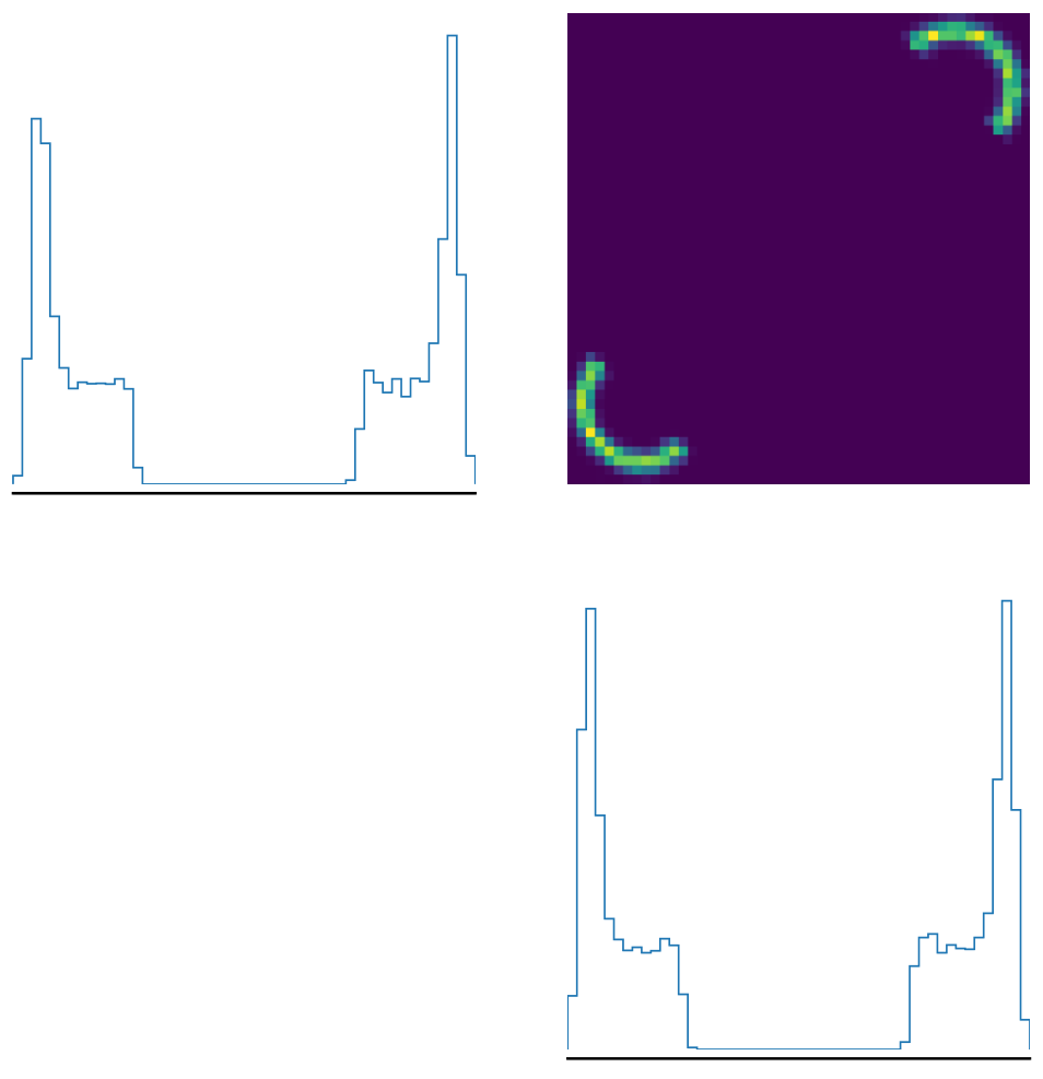
It was shown in (Nijkamp et al. 2019) that EBMs trained by replacing the intractable expectation under the EBM with an expectation under a particle approximation obtained by running parallel runs of Langevin Dynamics initialized from random noise and updated for a fixed (and small) amount of steps can yield an EBM whose density is not proportional to the true density, but rather a generative model that can generate faithful images by running a few steps of Langevin Dynamics from random noise on it. Our design choices for both training and inference purposefully avoid this effect from manifesting in UNLE. During training, we estimate the intractable expectation using persistent MCMC or SMC chains, e.g by initializing the MCMC (or SMC) algorithm of iteration with the result of the MCMC (or SMC) algorithm at iteration , yielding a different training method than short-run EBMs. At inference, the posterior model is sampled from Markov Chains with a significant burn-in period, contrasting with the sampling model of short-run EBMs. Figure 8 compares the density of UNLE’s posterior estimate for the Two Moons model (a 2D posterior which can be easily visualized) with the true posterior. As Figure 8 shows, AUNLE and SUNLE’s posterior density match the ground truth very closely, demonstrating that UNLE’s EBM is not a short-run generative model, but a faithful density estimator.

C.3 Validating the -uniformization of AUNLE’s posterior in practice
Proposition 3.1 ensures that the normalizing constant present AUNLE’s posterior is independent of provided that the problem is well-specified, and that , the optimum of AUNLE’s population objective. In practice, these conditions will not hold exactly, and the uniformization of AUNLE’s posterior thus only holds approximately. To assess the loss of precision associated with using a standard MCMC posterior in the context of approximate uniformization, we compare the quality of AUNLE’s posterior samples obtained using a standard MCMC sampler (which is valid only if uniformization holds), and using a doubly-intractable MCMC sampler, which handles non-uniformized posteriors. We mitigate the approximation error of doubly-intractable samplers by using a large number of steps (1000) when sampling from the likelihood using MCMC. As Figure 9 shows, there is no gain in using a doubly-intractable sampler for inference in AUNLE, suggesting that the uniformization property of AUNLE holds well in practice.
C.4 Computational Cost Analysis
Training unnormalized models using approximate likelihood is computationally intensive, as it requires running a sampler during training at each gradient step, yielding a computational cost of , where is the number of gradient steps, is the number of MCMC steps, and is the number of parallel chains used to estimate the gradient.
To maximize the efficiency of training, we implement all samplers using jax (Frostig et al. 2018), which provides a just-in-time compiler and an auto-vectorization primitive that generates efficient, custom parallel sampling routines. For AUNLE, we introduce a warm-started SMC approximation procedure to estimate gradients, yielding competitive performance with as little as 5 intermediate probabilities per gradient computation. For SUNLE, we warm-start the parameters of the EBM across training rounds, and warm-start the chains of the doubly-intractable sampler across inference rounds, which significantly reduces the need for burn-in steps and long training. Finally, all experiments are run on GPUs. Together, these techniques make AUNLE and SUNLE almost always the fastest methods for amortized and sequential inference, with total per-problem runtimes of 2 minutes for AUNLE and 15 minutes for SUNLE on benchmark models (which is significantly faster than NLE and SNLE on their canonical CPU setup, Lueckmann et al. 2021) and less than 3 hours for SUNLE on the pyloric network model (with half of this time spent simulating samples). The latter is 10 times faster than SNVI (30 hours) on the same model. A breakdown of training, simulation and inference time is provided in Figure 10. We note that (S)NLE was run on a CPU, which is the advertised computational setting (Lueckmann et al. 2021), as (S)NLE uses deep and shallow networks that do not benefit much from GPU acceleration.
We note that the time spent performing inference is negligible for AUNLE, which uses standard MCMC for inference thanks to the tilting trick employed in its model. On the other hand, the runtime of SUNLE, which performs inference using a doubly-intractable sampler is dominated by its inference phase. This point demonstrates the computational benefits of the AUNLE’s tilting trick. Note that SUNLE performs inference in a multi-round procedure, and requires thus training and inference phases (where is the number of rounds), as opposed to 1 for AUNLE. We alleviate this effect by leveraging efficient warm-starting strategies for both training and inference, which to an extent amortizes these steps across rounds.
C.5 Experimental setup for SNLE and SMNLE
SNLE
The results reported for SNLE are the one present in the SBI benchmark suite (Lueckmann et al. 2021), which reports the performance of both NLE and SNLE on all benchmark problems studied in this paper.
SMNLE
The results reported for SMNLE were obtained by running the implementation referenced by (Pacchiardi & Dutta 2022). SMNLE comes in two variants: the first variant uses standard Score Matching (Hyvärinen & Dayan 2005) to estimate its conditional EBM, while the second variant uses Sliced Score Matching (Song et al. 2020), which yields significant computational speedups during training. For both methods, we train the model using 500 epochs, and neural networks with 4 hidden layers and 50 hidden and outputs units. To optimize the inference performance, we carry out inference using our own doubly-intractable sampler, which automatically tunes all parameters of the doubly-intractable samplers except for the number of burn-in steps, and initializes the chain at local posterior modes. We carry out a grid search over the learning rates 0.01 and 0.001, and leave other training parameters to their default. Figures in the main body only report the performance of the Sliced Score Matching variant, which perform better in practice and run faster by an order of magnitude. Figure 11 reports the performance of both variants for completeness. We used GPUs for both training and inference in SMNLE, yielding similar or higher training compared to AUNLE when using the sliced variant, and much longer training times when using the standard variant.
C.6 Neuroscience Model: Details
Pairwise Marginals
We provide the full pairwise marginals obtained after computing a kernel density estimation on the final posterior samples of SUNLE. We retrieve similar patterns as the one displayed in the pairwise marginals of SNVI samples. We refer to (Glöckler et al. 2021) for more details on the specificities of this model.

Use of a Calibration Network
Due to the presence of invalid observations, we proceed as in (Glöckler et al. 2021) and fit a calibration network that allows to remove the bias induced by throwing away pairs of (parameters, observations) when the observations do not have well defined summary statistics. We use a similar architecture as in (Glöckler et al. 2021).