Controlled remote implementation of operations via graph states
Abstract
We propose protocols for controlled remote implementation of operations with convincing control power. Sharing a -partite graph state, participants collaborate to prepare the stator and realize the operation on unknown states for distributed systems , with the permission of a controller. All the implementation requirements of our protocol can be satisfied by means of local operations and classical communications, and the experimental feasibility is presented according to current techniques. We characterize the entanglement requirement of our protocol in terms of geometric measure of entanglement. It turns out to be economic to realize the control function from the perspective of entanglement cost. Further we show that the control power of our protocol is reliable by positive operator valued measurement.
I Introduction
As the unique resource, entanglement allows the emergence and development of quantum information processing, such as teleportation bennett1993teleport, dense coding bennett1992communication and cryptography gisin2002quantum; portmann2022security. Being expected to offer substantial speed-ups over classical counterparts, quantum computation has been paid a lot of attention deutsch1992rapid; shor1997polynomial. Several challenges have surfaced in its actual construction, such as decoherence and dissipation, sufficiently manipulating a large number of qubits, and undesirable interactions alexeew2021quantum. To counter such challenges, distributed quantum computation has been proposed cirac1999distributed; serafini2006distributed; cacciapuoti2020quantum. It requires to transfer states from one place to the other and implement the operations on a remote state faithfully. The first requirement has been met by quantum teleportation bennett1993teleport; pan1997experimental; georgescu202225years; qiu2022quantum. The second one has been tackled by remote implementation of operation (RIO) and controlled RIO (CRIO). RIO means that the quantum operation performed on the sender’s local system is able to act on an unknown state of a remote system that belongs to the receiver huelga2001quantum; huelga2002remote. Then CRIO was proposed by extending RIO to multipartite case with controller wang2007combined. The idea of that is to implement remote operations, but only with the permission of controller. It can definitely enhance the security of RIO. Both of RIO and CRIO play an important role not only in distributed quantum computation, but also other tasks in remote quantum information processing such as programming nielsen2000quantum, operation sharing wang2013determistic and remote state preparation bennett2001remote. They are realized by local operation and classical communication (LOCC) and consume entanglement resource. Some works concerning RIO have been presented and interesting progress has been made both theoretically reznik2002remote; chen2005probabilistic; wang2006remote; an2022joint and experimentally guo2005teleporting; huelga2005remote; bhaskar2020experimental. As for CRIO, it has been realized in terms of partially unknown quantum operations wang2007combined; he2014bidirectional, various classes of bipartite unitary operations yu2016implementation, arbitrary dimensional controlled phase gate gong2021control, and operators on different remote photon states an2022controlled. Entangled states including Bell, Greenberger-Horne-Zeilinger (GHZ), and five-qubit cluster states are employed as channels in these protocols. Theoretically, many of these protocols can hardly be scalable, or technically complicated. What’s more, the highly entangled states they employed are susceptible to noise, so it is a great challenge to realize them under experimental techniques.
In this paper, we propose CRIO protocols for the operations with convincing control power. The diagram of our protocol via a graph state is shown in FIG. 1. We generalize the protocol realizing RIO by stators reznik2002remote into CRIO. The stators in our protocol are constructed from shared graph states by LOCC, only with the permission of the controller. The protocol via a -partite graph state can be obtained by generalization, and that is used to implement remote operations on unknown states. Graph states are employed as the channel in our protocol for three reasons. Firstly, they make it possible to realize control function and enable our protocol to be scalable. Secondly, they are a natural resource for much of quantum information, and known to be most readily available multipartite resource in the laboratory bell2014experimental; yang2022sequential. Thirdly, many of the graph states show advantages for being robust to noise beriegel2001persistent. All the implementation requirements of our protocol can be satisfied by means of LOCC. The experimental feasibility is presented in terms of current techniques. The local operations and measurements can be implemented by a diamond nanophotonic resonator containing SiV quantum memory with an integrated microwave stripline bhaskar2020experimental. The entanglement requirement of our protocol is characterized in terms of geometric measure of entanglement. It is presented in Proposition 2. Compared with the former protocol in reznik2002remote, ours is endowed with control function, while it only requires the same entanglement resource. Hence it is economic to realize the control function from the perspective of entanglement cost. Besides, we analyze the control power in our protocol, and obtain that without the permission of the controller, other participants can hardly realize the remote implementation of operation. It is shown in Proposition 3. Thus the control power of our protocol is convincing. Our protocol shows advantage in stronger security, extensive applications, and advanced efficiency. It can contribute to improving the ability of distributed quantum computing and stimulate more research work on quantum information processing.

Graph states have a strong connection with quantum computation. Naturally, they can be characterized by geometric measure of entanglement (GM), a well-known entanglement measure for multipartite systems. GM not only provides a simple geometric picture, but also has significant operational meanings. It has connections with optimal entanglement witnesses wei2003geometric, and multipartite state discrimination under LOCC hayashi2006bounds. As one of the most widely used entanglement measures for the multipartite states, GM fulfills all the desired properties of an entanglement monotone wei2003geometric. It has been utilized to determine the universality of resource states for one-way quantum computation nest2007fundamentals. It also has been employed to show that most entangled states are too entangled to be useful as computational resources gross2009most.
The rest of this paper is organized as follows. In Sec. II, we introduce some basic concepts of graph states, GM and stator. Then we simply recall the deduction of eigenoperator equation of the stator. In Sec. III, we propose our CRIO protocol. We show the implementation of remote operation on an unknown state for a single system via a tripartite graph state in Sec. III.1. The protocol via a five-partite graph state is presented in Sec. III.2, which is slightly different from the former one and used to implement operations on two remote systems. Then we generalize it into the one via a -partite graph state in Sec. III.3. We show GM of the graph states used in our protocols in Sec. IV. We do the control power analysis in Sec. V, and exhibit the experimental feasibility of our protocol in Sec. VI. Finally, we conclude in Sec. VII.
II Preliminaries
In this section, we recall the definitions and some properties of graph states, GM and stator. In Sec. II.1, we recall the definition of graph states, and demonstrate a graph state with the help of quantum gates. In Sec. II.2, we recall the definition of GM and show a lemma we employ to characterize the GM of graph states. In Sec. II.3, we introduce the concept of stator, and present the eigenoperator equation of the stator used in this paper.
II.1 Graph states
A graph is a pair , where is the set of vertices and is the set of edges. With each graph, a graph state is associated. An axiomatic framework for mapping graphs to quantum states is proposed in ionicioiu2012encoding. A graph state is a certain pure state on a Hilbert space . Each vertex of the graph labels a qubit. Each vertex of the graph is attached to a Hermitian operator
| (1) |
Here and are the Pauli matrices and the upper index specifies the Hilbert space on which the operator acts. is an observable of the qubits related to vertex and all of its neighbors . There are operators in the set . The operators in this set are all commute.
We demonstrate a graph state with the help of Hadamard gate and two-qubit controlled-Z gate , where
| (2) |
and the gate
| (3) |
denotes the gate with control qubit and controlled qubit . By the two gates, we can show the preparation of graph states in the quantum circuit conveniently.
A graph state is created from a graph of vertices by assigning a qubit to each vertex and initializing them by applying the Hadamard gate on each qubit. Let . If two vertices are connected by an edge , then we perform over the initialized -qubit state . By implementing all the controlled-Z gates corresponding the edges , we obtain the graph state
| (4) |
Graph states are useful resources with applications spanning many aspects of quantum information processing, such as computation raussendorf2001a, cryptography qian2012quantum, quantum error correction liao2022topological and networks cuquet2012growth. Experimentally, different techniques have been studied to implement graph states including ion traps barreiro2011An, superconducting qubits song201710qubit, and continuous variable optics walschaers2018tailoring.
II.2 Geometric measure of entanglement
Geometric measure of entanglement (GM) is a well-known entanglement measure for multipartite systems wei2003geometric. It measures the closest distance in terms of overlap between a given state and the set of separable states, or the set of pure product states. Originally introduced for pure bipartite states, GM was subsequently generalized to multipartite and to mixed states. Several inequivalent definitions of GM has surfaced by now. In this paper, we shall follow the definition given in (5) and (6).
| (5) | |||||
| (6) |
Here SEP denotes the separable states and PRO denotes the fully pure product states in the Hilbert space . GM is known only for a few examples, such as bipartite pure states, GHZ-type states, antisymmetric basis states, pure symmetric three-qubit states and some graph states hayashi2008entanglement; markham2007entanglement; chen2010computation.
We show the following fact given in Ref. zhu2011additivity. It is a useful lemma concerning the closest product states of non-negative states. Here the closest product state denotes any pure product state maximizing (5). The non-negative state means that all its entries in the computational basis are non-negative.
Lemma 1
The closest product state to a non-negative state can be chosen to be non-negative.
The proof is presented in Lemma 8 of Ref. zhu2011additivity. This lemma can be used to characterize GM of the states that are non-negative or locally equivalent to non-negative states. In addition, it contributes to prove the strong additivity of GM of the states including Bell diagonal states, maximally correlated generalized Bell diagonal states, isotropic states, generalized Dicke states, mixture of Dicke states, the Smolin state and Dür’s multipartite entangled states.
II.3 Stator and eigenoperator equation
The stator, a hybrid state operator, is an object that expresses quantum correlations between states of one participant and operators of the other participant. It is firstly proposed in Ref. reznik2002remote to implement a class of operations on remote systems. Given a well-prepared stator, the operation on Bob’s system is remotely brought about by Alice’s local operations. The desired operation is determined by Alice and unknown to Bob. Hence it demonstrates advantage in terms of security.
A stator shared by remote observers Alice and Bob is in the space
| (7) |
where and are the Hilbert spaces of Alice and Bob respectively, and denotes the operators acting on an arbitrary state in . A stator has the general form
| (8) |
where , , , acts on states in and are complex numbers. For each stator, an eigenoperator equation can be constructed. We consider the following stator used in this paper,
| (9) |
Here , where is the axis vector and is the Pauli matrix vector. The states are the eigenstates of . One can verify that . Obviously, satisfies the eigenoperator equation
| (10) |
Thus for any analytic function , it also satisfies that
| (11) |
and particularly,
| (12) |
where is any real number determined by Alice. Using the stator, a unitary operation on Alice’s qubit gives rise to a similar unitary operation acting on Bob’s system, which is remote to Alice. The construction of stator and the implementation of remote operations are both realized by LOCC.
III Controlled remote implementation of operations
In this section, we show the implementation of controlled remote operations via a graph state. The participants share the entangled graph state as resource. They cooperate to realize the remote operations on unknown states for remote systems by applying LOCC. Here is the angle of rotation only known by participants and unknown to others including the controller. Besides, the controller takes the responsibility to decide whether or not and when the implementation of remote operations should be done on each system. Thus our protocol shows advantage in terms of strong security and extensive applications. In Sec. III.1, we introduce the implementation of operation on one remote system via a tripartite graph state. In Sec. III.2, we show the protocol via a five-partite graph state, where two operations are implemented on two remote systems respectively. In this protocol, appropriate local Hadamard operations are employed. So it is different from the protocol via tripartite state. Then we generalize this protocol into the one via a -partite graph state (). It is presented in Sec. III.3.
III.1 The protocol via a tripartite graph state
In this protocol, three participants Alice, Bob and Charlie locate in distributed places. Alice is the controller who decides whether and when the remote implementation of operation on system can be realized by Bob and Charlie. The diagram of this process is shown in FIG. 1. The three participants share the tripartite graph state
| (13) |
where qubits belong to Alice, Bob and Charlie, respectively. The entangled state is prepared by the circuit shown in FIG. III.1.
Given an unknown state for system , Bob and Charlie implement the remote unitary operation on system , only with the permission of the controller Alice. This process is completed by applying LOCC via the shared entangled state . Here is any real number determined by Bob, and system belongs to Charlie.
First, they construct the stator , this process is performed on the state . We do not show in each step for simplicity. Charlie performs the local operation on his qubits and , where
| (14) |
Here the operator acting on the system satisfies . So the stator is
| (15) | |||||
Now Alice’s qubit is correlated with qubits and . If Alice does not wish to cooperate with Bob and Charlie, she does nothing or something unknown to them. Then the relation between qubits and is unknown to Bob and Charlie and hence they can hardly construct the stator. Otherwise, if Alice wants the operations to be implemented, she performs a measurement of on qubit , and informs Bob of the measurement result. If the result is , Bob performs the operation on qubit , otherwise Bob need not perform any operation. They obtain the stator
| (16) |
Then Charlie measures qubit in the basis and . If the result is , Bob implements the operation on qubit , otherwise Bob does nothing. Hence they construct the following stator successfully,
| (17) |
The second step is to implement the operation on system , with the help of eigenoperator equation
| (18) |
Note that , so we have .
Now Bob and Charlie implement the remote operation by stator . Bob implements the operation on qubit . Based on Eq. (18), the resulting state is
| (19) | |||||
Bob measures qubit in the Z-basis and , and informs Charlie the result. If it is , Charlie performs the local rotation on system . This completes our CRIO protocol via .
III.2 The protocol via a five-partite graph state
In this protocol, we take the five-partite graph state as entanglement resource. The controller Alice in this protocol decides whether and when the work of the following two groups can be done. The first group consists of Bob and David who aim to realize the remote implementation of operations , and the second group include Charlie and Eve who aim to realize . They share the following graph state . For convenience of the measurement on qubit , we rearrange the state in the basis and ,
| (20) | |||||
where qubits belong to Alice, Bob, Charlie, David, and Eve respectively, and the preparation of this state is shown in FIG. III.2. For the operations and , and are real numbers determined by Bob and Charlie, respectively. System and belong to David and Eve respectively.
The first step is to construct the stator. For convenience, we ignore the global factor in the following statement. David and Eve perform the local operations and respectively, where
| (21) | |||||
| (22) |
This yields the stator
Next, Charlie performs the operation on qubit . Note that and . The stator becomes
From (III.2), one can find that Alice’s qubit is correlated with qubits and . If Alice does not wish to cooperate with the two groups, she does nothing or something unknown to them. Then the relation between qubits and is unknown to Bob and David and hence they can hardly construct the stator. So it does with Charlie and Eve. Otherwise, Alice wants the operations to be implemented then she implements the measurement of on qubit and informs Bob and Charlie of the result by classical communication. If the result is , Bob and Charlie perform the operation on qubit , otherwise they do nothing. Thus they obtain the stator
David and Eve perform the measurement of on qubit and , and send their measurement results to Bob and Charlie, respectively. The diagram of this process is shown in FIG. 4.

So they prepare the stator successfully, where
| (26) |
Next they implement the operations and on two unknown states and for system and , respectively. The relation can be established. Hence the stator also satisfies the following eigenoperator equation, which is similar to Eq. (18),
| (27) |
Bob and Charlie implement the operations and on their qubits and respectively. Based on Eq. (27), we obtain that the state is now
| (28) | |||||
Finally Bob and Charlie perform the measurement of on qubits and . Bob transmits the measurement result to David, and Charlie’s result sends to Eve. If the sender’s measurement result is , the receiver performs the operation (), otherwise the receiver need not perform any operation.
III.3 The protocol via a -partite graph state
We show the protocol via a -partite graph state, which is the generalization of the protocol in Sec. III.2. In this protocol, participants are involved. Participant is the controller who supervises distributed groups. Participants and work as a group to implement the operation on the unknown states for system , for . For each group, the real numbers and is only available to participants and , respectively. During this process, the controller determines whether and when these operations should be implemented, but knows nothing about the parameters of the operations. That is to say, none of the participants is able to obtain the complete information of the target operations. It guarantees the security of our protocol. The participants share the following -qubit graph state,
| (29) | |||||
where qubit belongs to participant respectively, for . The boolean function , for and ,
| (30) |
Here denotes plus modulo two, and
| (31) |
The state is prepared by the quantum circuit shown in FIG. III.3.


Now we show the realization of the remote operations by the cooperation of participants. First, they prepare the stator by LOCC, only with the permission of controller . The stators are constructed on the unknown states for remote systems . Second, the operations are implemented on these systems with the help of the stator. The construction of stator consists of four steps, i.e. STEP 1-4 in the following statement. In each step, the participants perform a kind of local operations or measurements. For convenience, we ignore the global factor in the following statement.
STEP 1: The participants perform the local operations
| (32) |
on the entangled state in (29) for qubit and system respectively, where . The operation satisfies that . The resulting stator is
| (33) | |||||
For convenience of the statement, we rearrange the stator according to qubit in the basis and as follows,
| (34) |
where and are boolean functions of :
| (35) | |||||
| (36) |
From Eqs. (35) and (36), one can obtain that when , and when . Hence, ignoring the global factor, the stator in (III.3) is equal to
| (37) |
where
| (38) | |||||
| (39) | |||||
Here and are boolean functions of :
| (40) | |||||
| (41) |
STEP 2: Participants perform the operation on their qubits , respectively.
To show the effect of the operation on the stator in (III.3) clearly, we rearrange in (38) and in (39) as follows,
| (42) | |||||
| (43) | |||||
For , it holds that
| (44) | |||
| (45) |
Applying (44), (45) to (42), (43) respectively, it yields the following stator . The global factor is ignored here,
| (46) | |||||
STEP 3: From (46), one can find that the controller’s qubit is correlated with qubits and , for . If the controller does not wish to cooperate with other groups including and , he does nothing or something unknown to other groups. Then the relation between qubits and is unknown to participants and and hence they cannot realize the operations at the beginning of this subsection. Otherwise, if the controller permits the realization of these operations, he implements the measurement of on qubit , and informs of the result. If the result is , the receivers perform on their qubits, otherwise they do nothing. This yields the stator
| (47) | |||||
STEP 4: Participants , ,…, measure their qubits in the X-basis, and inform of the results by classical communication, respectively. If the sender’s result is , the receiver performs the operation on his qubit, otherwise the receiver does nothing. So they construct the stator
| (48) | |||||
where .
Then the stator is employed to implement the remote operations on the unknown state for remote systems . Similar to the eigenoperator equation shown in (12), the equation for stator still holds,
| (49) |
where and is any real number determined by the participant . By performing the local operation on qubit , the participant realizes the corresponding operation on remote system . The implementation consists of two steps.
STEP 5: The participant performs the local operation on qubit , for . Using Eq. (49), the state is now
| (50) |
STEP 6: To eliminate the remaining stator on the state and only keep the target operation, the participant implements the measurement of on qubit , and informs of the measurement result, where . If the sender ’s result is , the receiver performs the operation , otherwise the receiver need not perform any operation. So they eliminate the stator . The resulting state is
| (51) |
It indicates that they have implemented the remote operation successfully.
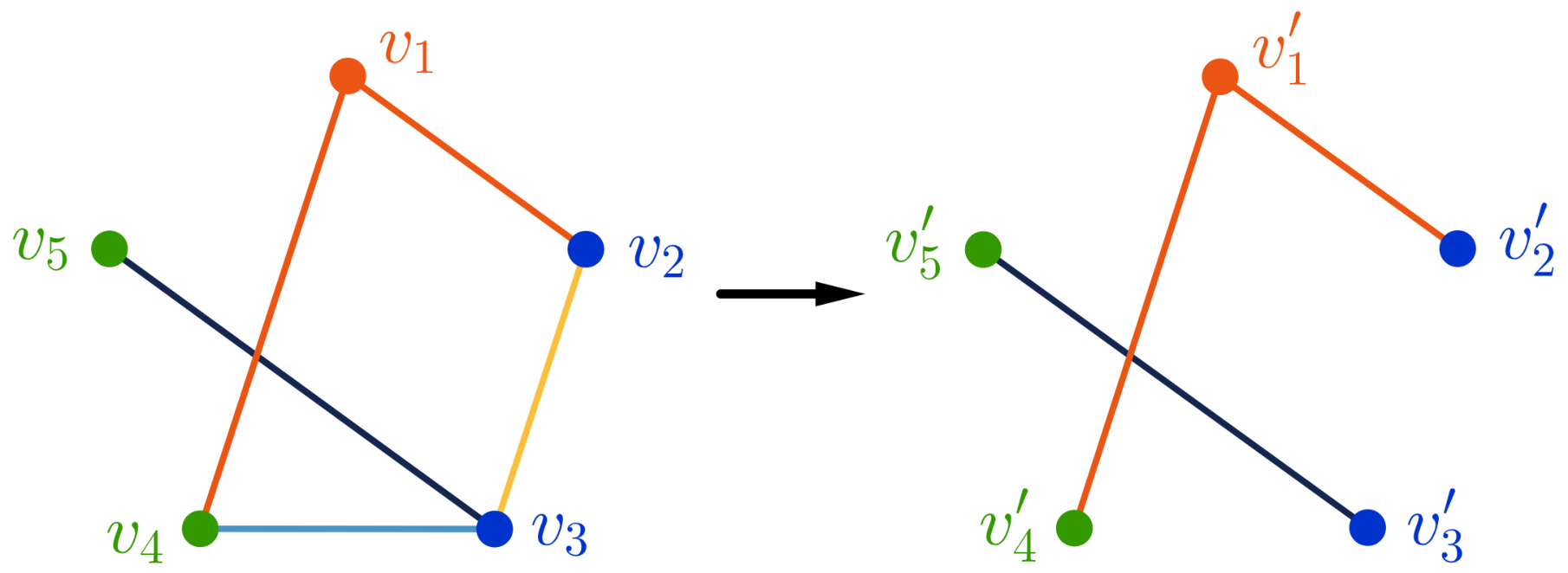
In our controlled protocol via , the controller is able to control each of the groups to implement operations on remote system , for . In fact, according to the demand of realistic background, the controller can control any of these groups, and discard the rest of groups with . It can be realized by employing appropriate graph states. Compared with the construction of in FIG. III.3 and 6, such states can be constructed by removing corresponding gates and in pairs, for . We take the protocol via as an example. In the former protocol presented in Sec. III.2, the controller can control both groups. Now we assume the controller only wants to control the group consisting of participants and . This task can be realized by employing another graph state . The construction of can be done with the help of the graph on the right hand side in FIG. 7. That is to say, can be constructed by removing the gates and compared with the construction of state . From this point of view, our protocol can flexibly follow the actual demands and thus it shows advantage in extensive applications.
IV geometric measure of entanglement for graph states
In this section, we investigate the GM of the graph states used in this paper. Then we compare the entanglement requirement between the protocol in Ref. reznik2002remote and our protocol. We find that the two protocols require the same entanglement resource. Hence it is economic to realize the control function from the perspective of entanglement cost.
First we show an example by considering the tripartite graph state shown in (III.1). Since the local unitary operations do not change the entanglement of the states, we perform the local Hadamard gate on qubit of , and obtain the state
| (52) |
Now we consider the GM of . According to Lemma 1, its closest product state can be chosen to be non-negative. Let be a closest product state, with . After some calculations, we obtain that
| (53) | |||||
| (54) |
The maximum in the above equation is obtained at , i.e. .
Next we consider the GM of ()-partite graph state in (29). We show the following fact:
Proposition 2
The geometric measure of entanglement for the state is equal to , for .
Proof.
We reduce the state by applying the local Hadamard gates on qubits . Then it can be transformed to the following non-negative state,
| (55) | |||||
So the GM of is equal to that of . Let and . We denote as . Obviously, we have
| (56) |
where and . Using (56), we obtain that
| (57) | |||||
By some calculations, we have
| (58) |
Using Lemma 1, we have with . From (58), the value of reaches the maximum when . Hence we have
It holds that
| (59) |
Now we compare the entanglement requirement between the protocol in Ref. reznik2002remote and our controlled protocol in terms of GM. The protocol for remote operations by stator is firstly proposed in Ref. reznik2002remote. In this protocol, participants share the -partite entangled state to realize the remote operations on systems without the controller. The entangled states used in that protocol are given as follows,
| (60) | |||||
| (61) | |||||
| (62) |
We investigate GM of the states in (60)-(62) and list the entangled states required in the two protocols for a given number of systems. The results are presented in TABLE. 1.
| Controlled remote implementation protocol in this paper | Remote implementation protocol in Ref. reznik2002remote | |||
| Number of systems | Entangled state | GM | Entangled state | GM |
| 1 | in (III.1) | 1 | in (60) | 1 |
| 2 | in (III.2) | 2 | in (61) | 2 |
| ⋮ | ⋮ | ⋮ | ⋮ | ⋮ |
| for any integer | in (29) | in (62) | ||
From TABLE. 1, we see that the protocol we proposed in this paper requires the same entanglement resource as the former protocol in Ref. reznik2002remote. That is to say, although one ”controller” who enables control over other groups is added in our protocol, the entanglement cost of our protocol does not increase. Hence it is economic to realize the control function from the perspective of entanglement cost.
V control power analysis
In this section, we show the control power analysis of our controlled protocol. In analogy to the control power of quantum teleportation li2015analysis, the controller’s power here is determined by the situation that the remote operation be accomplished without the controller’s help. If the controller does not wish the remote operation to be executed, he will not perform the measurement and other participants can hardly realize the target operations on remote systems. We show that without the controller’s permission, eight specified operations can be implemented with the success rate of 50%, other operations can be realized with the success rate of 25%. It means that the control power is reliable in our controlled remote implementation protocol. The main result of this section is shown in Proposition 3.
We consider the protocol via in Sec. III.1. Other protocols can be analyzed in the same way, as the result we obtained in this section is valid for each group in the protocol via . To implement the remote operation without the controller Alice’s help, Bob and Charlie collaborate to perform some POVM measurement on qubits and to eliminate the entanglement between qubit and . In particular, Bob carries out the POVM and Charlie carries out , for . The operators satisfy two basic restrictions,
| (63) | |||
| (64) |
We investigate the probability by which POVM operators and occur in the measurement. It is denoted as . We normalize the stator in (III.1) and define the normalized stator as , where
| (65) |
Note that . So we have
| (66) | |||||
That is to say, the probability of performing on qubits and is equal to 25% for any .
Suppose and . Without loss of generality, we assume and . Let with , i.e.
| (67) | |||||
| (68) | |||||
| (69) | |||||
| (70) |
We consider the situation that POVM operators and occur in the measurement, for . After the measurement, the stator in (III.1) becomes
| (71) | |||||
Bob and Charlie aim to implement the operation
| (72) |
on system without Alice’s help. Their goal is to make qubit separate from remaining qubits and by POVM measurement. We analyze the possible angle in the operation that can be realized in this scheme, and obtain the following fact:
Proposition 3
For the protocol via in Sec. III.1, the probabilistic implementation of remote operation can be realized by POVM measurement without controller’s permission. The success rate to realize the operation is equal to 50% for , and that is equal to 25% for .
Now we show some security analysis of the POVM measurement scheme. In our controlled protocol in Sec. III.1, the deterministic implementation of can be realized with the permission of controller Alice. The rotation angle can be chosen as any value and Charlie is unaware of any information of the operation that Bob wants to implement. However, in this POVM measurement scheme in Sec. V, we claim that Charlie can obtain the value of with the probability of or 12.5%. It means that the confidentiality of remote operation may be destroyed. In fact, the rotation angle in can only be one of { with } and { with } when Charlie prepares the POVM operators with and , respectively. So there are four possible rotation angles for a group of POVM operators with given parameters. Charlie may guess what the rotation angle is, and get to the correct answer with the probability of 25%. When Charlie prepares the operator with , the target rotation angle can only be one of , so Charlie may be aware of the value of with the probability of 12.5%.
To sum up, Bob and Charlie can hardly realize the remote implementation of operation perfectly without the permission of controller Alice. The control power in our controlled protocol is convincing.
VI experimental feasibility
As the entanglement resource of our protocol, graph states are the most readily available multipartite resource in the laboratory, and they have already been built and used for information processing experimentally. In a recent work, the deterministic protocol is implemented, by which the GHZ states of up to 14 photons and linear cluster states of up to 12 photons have been grown with a fidelity lower bounded by 76(6)% and 56(4)%, respectively thomas2022efficient. A scheme to prepare an ultrahigh-fidelity four-photon linear cluster state has been proposed, and it has been experimentally demonstrated with the fidelity of 0.9517 0.0027. This scheme can be directly extended to more photons to generate an N-qubit linear cluster state zhang2016experimental. Recently, an efficient scheme is demonstrated to prepare graph states with only a polynomial overhead using long-lived atomic quantum memories zhang2022quantum. Such technique can be used to prepare the graph states (29) in our protocol, so the requirement of entanglement resource can be satisfied.
Remote implementation has been demonstrated theoretically and realized experimentally, such as remote state preparation pogorzalek2019secure, nonlocal CNOT operation implementation zhou2019hyper and remote generation of entanglement morin2014remote. In our controlled remote implementation protocol, the participants prepare the stators and implement the remote operation by applying LOCC on shared entangled state. The local operations and measurements required in our protocol are operations and X-basis, Z- basis measurements, respectively. In the work presented in bhaskar2020experimental, a kind of memory-enhanced quantum communication is demonstrated experimentally. In this work, some local operations and measurements in the X and Z bases are implemented with a time-delay interferometer (TDI). The device consists of a diamond nanophotonic resonator containing SiV quantum memory with an integrated microwave stripline. By reducing the possibility that an additional photon reaches the cavity, high spin-photon gate fidelities are enabled. Measurements are performed with high-fidelity by keeping track of the timing when the TDI piezo voltage reaches a limiting value, which guarantees that the SiV is always resonant with the photonic qubits. The experimental technique in this work can be employed to realize our protocol. Hence our protocol is feasible according to the present experimental technologies. Additionally, the memory-based communication nodes allow asynchronous Bell-state measurement and it may enhance the performance of our protocol experimentally.
VII conclusion
We have proposed the protocol for controlled remote implementation of operations in the form of for each system. A family of graph states is constructed as the entanglement resource in our protocol. Sharing the -partite graph state as channel, participants are able to realize the remote operations on unknown states for distant systems respectively, only with the permission of a controller. The implementation requirements of our protocol can be satisfied only by means of LOCC. Further we have characterized GM of the graph states in our protocol. Compared with the entanglement requirement of the protocol in reznik2002remote, the control function of our protocol is realized economically. Based on the result of control power analysis, the control power is reliable in our protocol, i.e. others can hardly realize the implementation without the permission of controller. Further we have exhibited the experimental feasibility of our protocol in terms of current techniques.
Many problems arising from this paper can be further explored. As we all know, multilevel systems as qudits feature more advantages than their binary counterpart. Our protocol can be considered in high-dimensional Hilbert spaces, and may be used to implement some other operations. The protocol with more controllers for specific systems can be studied by applying appropriate graph states and local implementations. The interaction between quantum states and environment is unavoidable, leading to the loss of accuracy. Considering the situation that graph states in our protocol are affected by noise, the probabilistic implementation of that can be developed.
ACKNOWLEDGMENTS
We thank Li Yu, Jun Li and Zhaohui Wei for careful reading of the whole paper. The authors were supported by the NNSF of China (Grant No. 11871089) and the Fundamental Research Funds for the Central Universities (Grant No. ZG216S2005).
AUTHOR CONTRIBUTIONS
All authors contributed to the discussion of results and writing of the manuscript.
COMPETING INTERESTS
The authors declare no competing interests.
Appendix A control power analysis in terms of POVM measurement
Proof.
The proof includes two parts: first we consider case I for or in TABLE 2 in Sec. A.1, then we consider case II for in TABLE 3 in Sec. A.2, where with are defined in (67)-(70).
For other cases, the entanglement may not be eliminated or the same results are obtained as that in the former two cases. Case III for can be analyzed by the same way as case II and the same results are obtained, as the two cases both require two sets of coefficients and to be proportional, i.e. in case II and in case III. In case IV for and case V for , the entanglement can be eliminated only when with , which is included in case II.
A.1 Case I : or
The first case that or corresponds to or in (67)-(70), respectively. In this case, the operations with can be realized by TABLE 2, and the success rate of realization is equal to 50%.
As an example, the operations with or and or can be realized by different combinations of POVM operators. Bob and Charlie prepare the POVM operators with the parameters , and . Their POVM operators are
| (73) |
When the POVM operators occurs in the measurement, the stator in (V) becomes , where
| (74) | |||||
| (75) | |||||
| (76) | |||||
| (77) |
Note that , and . Hence, the operation with rotation angle or can be realized when and occur in the measurement; the operation with rotation angle or can be realized when and occur in the measurement. From (V), each of the four combinations of POVM operators occurs with the probability of . So Bob can only implement his desired operation with the success rate of 50%. For example, Bob wishes to implement the operation on system , he can only carry it off when the POVM operators and occur, and the probability of that is 50%.
The operations with or and or can also be realized by other POVM operators with different parameters. The process of implementation is the same as that of the former example. Combined with (63) and (67)-(70), we obtain the possible parameters in Bob and Charlie’s POVM operators and its corresponding rotation angle in that can be realized. They are shown in TABLE 2. Each of the four combinations of POVM operators , occurs with the same probability of , for . In this case, Bob can realize his desired operation with the probability of 50%, and his target operation can only be with the rotation angle , for .
| parameters in Bob’s POVM operator | parameters in Charlie’s POVM operator | POVM operators | coefficients in (V) | rotation angle in | |||||||||
| [0,] | 0 | 0 | 0 | 0 or | |||||||||
| 0 | 0 | or | |||||||||||
| 0 | 0 | 0 or | |||||||||||
| 0 | 0 | or | |||||||||||
| [0,] | 0 | 0 | 0 | or | |||||||||
| 0 | 0 | 0 or | |||||||||||
| 0 | 0 | or | |||||||||||
| 0 | 0 | 0 or | |||||||||||
A.2 Case II:
Next we consider the second case that , i.e. in (67)-(70). We set and with here, as they have been discussed in the former case. To eliminate the entanglement between qubit and , the coefficients in (V) should satisfy the following restriction,
| (78) |
where is a constant. So the stator in (V) becomes
| (79) |
The target operation that Bob and Charlie try to implement on system is . So the coefficients in (79) should satisfy
| (80) |
where is a constant with or , . From (67)-(70), (78) and (80), we obtain that
| (81) | |||||
| (82) | |||||
| (83) | |||||
| (84) |
Now we analyze the possible angle that satisfies the conditions above. Note that . From (81)-(84), we have
| (85) |
So we have and thus
| (86) | |||
| (87) |
Then from (83) and (86), we have
| (88) |
or
| (89) |
Obviously, . Note that and thus . Hence , i.e. . From (82), we have
| (90) |
Using (82), (83) and (87), we have
| (91) |
From (63), (64), (86), (87) and (90), we obtain that
| (92) | |||
| (93) |
Considering the restrictions (86), (87), (90)-(93) on Eqs. (82) and (83), we show that the remote operation with the rotation angle
| (94) |
can be realized with the success rate of 25%, and the operations corresponding to
| (95) |
can be realized with the success rate of 50%. The implementation of these operations with can be realized by TABLE 3.
As an example, Bob wants to realize the operation with . For this purpose, Bob and Charlie choose the POVM operators with the parameters , and , , respectively. Their POVM operators are
| (96) | |||
| (97) |
When the POVM operators occurs in the measurement, the stator in (79) becomes , where
| (98) | |||||
| (99) | |||||
| (100) | |||||
| (101) |
Note that and . When the POVM operators , , , occur, the operation with can be realized respectively, where or , or . Bob’s goal is to implement the operation with . It can only be realized when or occur. From (V), each of the four combinations of POVM operators occurs with the same probability of , for . So the success rate of realizing Bob’s target operation is 50%.
Other possible POVM operators with different parameters and its corresponding rotation angle in the operation are listed in TABLE 3. For the first set of POVM operators with parameter , Bob can realize his desired operation with the probability of 50% and the target operation that Bob can choose is with with . By the second set of operators with , the operation with can be realized. If Bob wants to implement that operation, he informs Charlie to prepare the POVM operators with four parameters: , , , where
| (102) |
| parameters in Bob’s POVM operators | parameters in Charlie’s POVM operators | success rate | POVM operators | coefficients in (79) | rotation angle in | ||||||||
| or | |||||||||||||
| 0 | 50% | 1 | or | ||||||||||
| 1 | or | ||||||||||||
| -1 | or | ||||||||||||
| -1 | or | ||||||||||||
| 0 | 25% | 1 | or | ||||||||||
| 1 | or | ||||||||||||
| -1 | or | ||||||||||||
| -1 | or | ||||||||||||
The operation with can be realized only when the operators occur in the measurement, respectively. From (V), each of the combination of POVM operators occurs with the probability of 25%. So the success rate is equal to 25%.
To conclude, we have shown that how Bob and Charlie implement the remote operation in the POVM measurement scheme without the permission of controller Alice. They can realize the operation of with the success rate of 50%, and the operation corresponding to can be realized with the success rate of 25%.
DATA AVAILABILITY
All relevant data supporting the main conclusions and figures of the document are available upon reasonable request. Please refer to Xinyu Qiu at xinyuqiu@buaa.edu.cn.
References
- [1] Bennett, Brassard, Crepeau, Jozsa, Peres, and Wootters. Teleporting an unknown quantum state via dual classical and einstein-podolsky-rosen channels. Physical review letters, 70(13):1895–1899, 1993.
- [2] Bennett and Wiesner. Communication via one- and two-particle operators on einstein-podolsky-rosen states. Physical review letters, 69(20):2881–2884, 1992.
- [3] Nicolas Gisin, Grégoire Ribordy, Wolfgang Tittel, and Hugo Zbinden. Quantum cryptography. Reviews of Modern Physics, 74:145–195, 2002.
- [4] Christopher Portmann and Renato Renner. Security in quantum cryptography. Reviews of Modern Physics, 94:025008, 2022.
- [5] Deutsch D. and Jozsa R. Rapid solution of problems by quantum computation. Proceedings of the Royal Society A: Mathematical, 439(1907):553–558, 1992.
- [6] Peter W. Shor. Polynomial-time algorithms for prime factorization and discrete logarithms on a quantum computer. Siam Journal on Computing, 1997.
- [7] Yuri Alexeev, Dave Bacon, Kenneth R. Brown, Robert Calderbank, Lincoln D. Carr, Frederic T. Chong, Brian DeMarco, Dirk Englund, Edward Farhi, Bill Fefferman, Alexey V. Gorshkov, Andrew Houck, Jungsang Kim, Shelby Kimmel, Michael Lange, Seth Lloyd, Mikhail D. Lukin, Dmitri Maslov, Peter Maunz, Christopher Monroe, John Preskill, Martin Roetteler, Martin J. Savage, and Jeff Thompson. Quantum computer systems for scientific discovery. PRX Quantum, 2:017001, 2021.
- [8] J. I. Cirac, A. K. Ekert, S. F. Huelga, and C. Macchiavello. Distributed quantum computation over noisy channels. Physical Review A, 59:4249–4254, 1999.
- [9] Alessio Serafini, Stefano Mancini, and Sougato Bose. Distributed quantum computation via optical fibers. Physical Review Letters, 96:010503, 2006.
- [10] Angela Sara Cacciapuoti, Marcello Caleffi, Francesco Tafuri, Francesco Saverio Cataliotti, Stefano Gherardini, and Giuseppe Bianchi. Quantum internet: Networking challenges in distributed quantum computing. IEEE Network, 34(1):137–143, 2020.
- [11] Dik Bouwmeester, Jian-Wei Pan, Klaus Mattle, Manfred Eibl, Harald Weinfurter, and Anton Zeilinger. Experimental quantum teleportation. Nature, 390(6660):575–579, 1997.
- [12] Iulia Georgescu. 25 years of experimental quantum teleportation. Nature Reviews Physics, 2022.
- [13] Xinyu Qiu and Lin Chen. Quantum cost of dense coding and teleportation. Physical Review A, 105:062451, 2022.
- [14] S. F. Huelga, J. A. Vaccaro, A. Chefles, and M. B. Plenio. Quantum remote control: Teleportation of unitary operations. Physical Review A, 63(4), 2001.
- [15] S. F. Huelga, M. B. Plenio, and J. A. Vaccaro. Remote control of restricted sets of operations: Teleportation of angles. Physical Review A, 65(4), 2002.
- [16] An Min Wang. Combined and controlled remote implementations of partially unknown quantum operations of multiqubits using greenberger-horne-zeilinger states. Physical Review A, 75(6), 2007.
- [17] M. A. Nielsen and I. L. Chuang. Quantum Computation and Quantum Information. Cambridge University Press, Cambridge, 2000.
- [18] Shengfang Wang, Yimin Liu, Jianlan Chen, Xiansong Liu, and Zhanjun Zhang. Deterministic single-qubit operation sharing with five-qubit cluster state. Quantum Information Processing, 12(7):2497–2507, 2013.
- [19] Charles H. Bennett, David P. DiVincenzo, Peter W. Shor, John A. Smolin, Barbara M. Terhal, and William K. Wootters. Remote state preparation. Physical Review Letters, 87:077902, 2001.
- [20] Benni Reznik, Yakir Aharonov, and Berry Groisman. Remote operations and interactions for systems of arbitrary-dimensional hilbert space: State-operator approach. Physical Review A, 65:032312, 2002.
- [21] Lin Chen and Yi-Xin Chen. Probabilistic implementation of a nonlocal operation using a nonmaximally entangled state. Physical Review A, 71(5), 2005.
- [22] An Min Wang. Remote implementations of partially unknown quantum operations of multiqubits. Physical Review A, 74(3), 2006.
- [23] Nguyen Ba An. Joint remote implementation of operators. Journal of Physics A: Mathematical and Theoretical, 55(39):395304, 2022.
- [24] Guo-Yong Xiang, Jian Li, and Guang-Can Guo. Teleporting a rotation on remote photons. Physical Review A, 71(4):044304.
- [25] Susana F. Huelga, Martin B. Plenio, Guo-Yong Xiang, Jian Li, and Guang-Can Guo. Remote implementation of quantum operations. Journal of Optics B: Quantum and Semiclassical Optics, 7(10):S384–S391, 2005.
- [26] M. K. Bhaskar, R. Riedinger, B. Machielse, D. S. Levonian, C. T. Nguyen, E. N. Knall, H. Park, D. Englund, M. Loncar, D. D. Sukachev, and M. D. Lukin. Experimental demonstration of memory-enhanced quantum communication. Nature, 580(7801):60–64, 2020.
- [27] Yan-He He, Qiu-Chun Lu, Yue-Ming Liao, Xing-Chen Qin, Jian-Sheng Qin, and Ping Zhou. Bidirectional controlled remote implementation of an arbitrary single qubit unitary operation with epr and cluster states. International Journal of Theoretical Physics, 54(5):1726–1736, 2014.
- [28] Li Yu and Kae Nemoto. Implementation of bipartite or remote unitary gates with repeater nodes. Physical Review A, 94:022320, 2016.
- [29] Neng-Fei Gong, Tie-Jun Wang, and Shohini Ghose. Control power of a high-dimensional controlled nonlocal quantum computation. Physical Review A, 103:052601, 2021.
- [30] Nguyen Ba An and Bich Thi Cao. Controlled remote implementation of operators via hyperentanglement. Journal of Physics A: Mathematical and Theoretical, 55(22), 2022.
- [31] B. A. Bell, D. A. Herrera-Marti, M. S. Tame, D. Markham, W. J. Wadsworth, and J. G. Rarity. Experimental demonstration of a graph state quantum error-correction code. Nature Communications, 5:3658, 2014.
- [32] Chao-Wei Yang, Yong Yu, Jun Li, Bo Jing, Xiao-Hui Bao, and Jian-Wei Pan. Sequential generation of multiphoton entanglement with a rydberg superatom. Nature Photonics, 16(9):658–661, 2022.
- [33] Hans J. Briegel and Robert Raussendorf. Persistent entanglement in arrays of interacting particles. Physical Review Letters, 86:910–913, 2001.
- [34] Tzu-Chieh Wei and Paul M. Goldbart. Geometric measure of entanglement and applications to bipartite and multipartite quantum states. Physical Review A, 68:042307, 2003.
- [35] M. Hayashi, D. Markham, M. Murao, M. Owari, and S. Virmani. Bounds on multipartite entangled orthogonal state discrimination using local operations and classical communication. Physical Review Letters, 96:040501, 2006.
- [36] M. Van den Nest, W. Dür, A. Miyake, and H. J. Briegel. Fundamentals of universality in one-way quantum computation. New Journal of Physics, 9(6):204–204, 2007.
- [37] D. Gross, S. T. Flammia, and J. Eisert. Most quantum states are too entangled to be useful as computational resources. Physical Review Letters, 102:190501, 2009.
- [38] Radu Ionicioiu and Tim P. Spiller. Encoding graphs into quantum states: An axiomatic approach. Physical Review A, 85:062313, 2012.
- [39] Robert Raussendorf and Hans J. Briegel. A one-way quantum computer. Physical Review Letters, 86:5188–5191, 2001.
- [40] Yujing Qian, Zhean Shen, Guangqiang He, and Guihua Zeng. Quantum-cryptography network via continuous-variable graph states. Physical Review A, 86:052333, 2012.
- [41] Pengcheng Liao, Barry C. Sanders, and David L. Feder. Topological graph states and quantum error-correction codes. Physical Review A, 105:042418, 2022.
- [42] Marti Cuquet and John Calsamiglia. Growth of graph states in quantum networks. Physical Review A, 86:042304, 2012.
- [43] Julio T. Barreiro, Markus Miiller, Philipp Schindler, Daniel Nigg, Thomas Monz, Michael Chwalla, Markus Hennrich, Christian F. Roos, Peter Zoller, and Rainer Blatt. An open-system quantum simulator with trapped ions. Nature, 470(7335):486–91, 2011.
- [44] Chao Song, Kai Xu, Wuxin Liu, Chui-ping Yang, Shi-Biao Zheng, Hui Deng, Qiwei Xie, Keqiang Huang, Qiujiang Guo, Libo Zhang, Pengfei Zhang, Da Xu, Dongning Zheng, Xiaobo Zhu, H. Wang, Y.-A. Chen, C.-Y. Lu, Siyuan Han, and Jian-Wei Pan. 10-qubit entanglement and parallel logic operations with a superconducting circuit. Physical Review Letters, 119:180511, 2017.
- [45] Mattia Walschaers, Supratik Sarkar, Valentina Parigi, and Nicolas Treps. Tailoring non-gaussian continuous-variable graph states. Physical Review Letters, 121:220501, 2018.
- [46] Masahito Hayashi, Damian Markham, Mio Murao, Masaki Owari, and Shashank Virmani. Entanglement of multiparty-stabilizer, symmetric, and antisymmetric states. Physical Review A, 77:012104, 2008.
- [47] Damian Markham, Akimasa Miyake, and Shashank Virmani. Entanglement and local information access for graph states. New Journal of Physics, 9(6):194–194, 2007.
- [48] Lin Chen, Aimin Xu, and Huangjun Zhu. Computation of the geometric measure of entanglement for pure multiqubit states. Physical Review A, 82:032301, 2010.
- [49] Huangjun Zhu, Lin Chen, and Masahito Hayashi. Additivity and non-additivity of multipartite entanglement measures. New Journal of Physics, 13(1):019501, 2011.
- [50] Xi-Han Li and Shohini Ghose. Analysis of -qubit perfect controlled teleportation schemes from the controller’s point of view. Physical Review A, 91:012320, 2015.
- [51] P. Thomas, L. Ruscio, O. Morin, and G. Rempe. Efficient generation of entangled multiphoton graph states from a single atom. Nature, 608(7924):677–681, 2022.
- [52] Chao Zhang, Yun-Feng Huang, Bi-Heng Liu, Chuan-Feng Li, and Guang-Can Guo. Experimental generation of a high-fidelity four-photon linear cluster state. Physical Review A, 93(6), 2016.
- [53] Sheng Zhang, Yu-Kai Wu, Chang Li, Nan Jiang, Yun-Fei Pu, and Lu-Ming Duan. Quantum-memory-enhanced preparation of nonlocal graph states. Physical Review Letters, 128:080501, 2022.
- [54] S. Pogorzalek, K. G. Fedorov, M. Xu, A. Parra-Rodriguez, M. Sanz, M. Fischer, E. Xie, K. Inomata, Y. Nakamura, E. Solano, A. Marx, F. Deppe, and R. Gross. Secure quantum remote state preparation of squeezed microwave states. Nature Communications, 10(1):2604, 2019.
- [55] P. Zhou and L. Lv. Hyper-parallel nonlocal cnot operation with hyperentanglement assisted by cross-kerr nonlinearity. Scientific Reports, 9(1):15939, 2019.
- [56] Olivier Morin, Kun Huang, Jianli Liu, Hanna Le Jeannic, Claude Fabre, and Julien Laurat. Remote creation of hybrid entanglement between particle-like and wave-like optical qubits. Nature Photonics, 8(7):570–574, 2014.