Environment-Aware AUV Trajectory Design and Resource Management for Multi-Tier Underwater ComputingThanks: This work of Jingjing Wang was supported in part by the National Natural Science Foundation of China under grant No. 62071268 and grant No. 6222101, in part by the Young Elite Scientist Sponsorship Program by the China Association for Science and Technology under Grant No. 2020QNRC001, and in part by the Fundamental Research Funds for the Central Universities. T. Bai was supported in part by the National Natural Science Foundation of China under Grant 62101015. Y. Deng was partially supported by Engineering and Physical Sciences Research Council (EPSRC), U.K., under Grant EP/W004348/1. Y. Ren was supported in part by the National Natural Science Foundation of China under grant No. 62127801, in part by the National Key R &D Program of China under Grant 2020YFD0901000, and in part by the project ‘The Verification Platform of Multi-tier Coverage Communication Network for Oceans (LZC0020)’ of Peng Cheng Laboratory. Moreover, L. Hanzo would like to acknowledge the financial support of the Engineering and Physical Sciences Research Council projects EP/W016605/1 and EP/P003990/1 (COALESCE) as well as of the European Research Council’s Advanced Fellow Grant QuantCom (Grant No. 789028). (Corresponding author: Jingjing Wang.)Thanks: X. Hou is with the Department of Electronic Engineering, Tsinghua University, Beijing, 100084, China. (E-mail: xiangwanghou@163.com.)Thanks: J. Wang and T. Bai are with the School of Cyber Science and Technology, Beihang University, Beijing 100191, China. (E-mail: drwangjj@buaa.edu.cn, tongbai@buaa.edu.cn.)Thanks: Y. Deng is with the Department of Engineering, King’s College London, London WC2R 2LS, U.K. (E-mail: yansha.deng@kcl.ac.uk.)Thanks: Y. Ren is with the Department of Electronic Engineering, Tsinghua University, Beijing, 100084, China, and also with the Network and Communication Research Center, Peng Cheng Laboratory, Shenzhen, 518055, China (E-mail: reny@tsinghua.edu.cn.)Thanks: L. Hanzo is with the School of Electronics and Computer Science, University of Southampton, Southampton, SO17 1BJ, UK. (E-mail: lh@ecs.soton.ac.uk.)

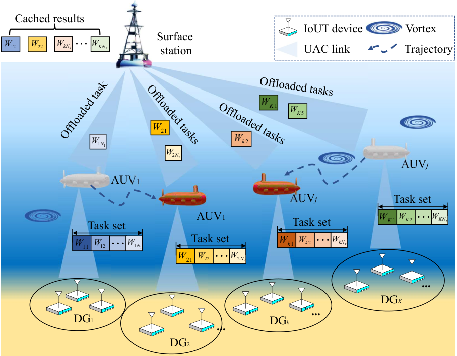
Fig. 1 shows our MTUC architecture, where multiple AUVs communicating with surface-stations perpetually cruising to provide computing service for a set of IoUT devices distributed in several device groups (DGs). Each AUV starts from the point of origin sight below the surface-station, and supports the assigned DGs in turn. We assume that there is a single surface-station, $M$ AUVs, and $K$ DGs. The $M$ AUVs are denoted by the set $\bm{AUV}=\{AUV_{1},{AUV}_{2},\ldots,{AUV}_{M}\}$, while the $K$ DGs are represented by the set $\bm{DG}=\{{{DG}}_{1},{{DG}}_{2},\ldots,{{DG}}_{K}\}$. Let us assume that there are a total of ${{N}_{k}}$ IoUT devices located in ${{DG}}_{k}$, which are represented by a set $\bm{{ND}_{k}}=\{{{n}_{{{k}_{1}}}},{{n}_{{{k}_{2}}}},\ldots,{{n}_{{{k}_{{N}_{k}}}}}\}$. For brevity, let $\bm{M}=\{1,2,\ldots,M\}$ represent the subscript of the AUVs, while $\bm{K}=\{1,2,\ldots,K\}$ the subscript of the DGs, and $\bm{{N}_{k}}=\{1,2,\ldots,{N}_{k}\}$ as the subscript of the IoUT devices located in DG_k. Let furthermore $\bm{P}_{\textrm{SS}}=(0,0,H)$, $\bm{P}_{j}^{\textrm{A}}=\left(x_{j}^{\textrm{A}},y_{j}^{\textrm{A}},d_{0}\right)$, $\bm{P}_{k}^{\textrm{DG}}=\left(x_{k}^{\textrm{DG}},y_{k}^{\textrm{DG}},z_{k}^{\textrm{DG}}\right)$ and $\bm{P}_{ki}^{\textrm{S}}=\left(x_{ki}^{\textrm{S}},y_{ki}^{\textrm{S}},h_{0}\right)$ represent the three-dimensional (3D) Euclidean coordinates of the surface-station, ${AUV}_{k}$, ${{DG}}_{k}$, and IoUT device ${{n}_{{{k}_{i}}}}$ located in ${{DG}}_{k}$, respectively.

We assume that each IoUT device has a task that has to be solved. The task generated by IoUT device ${{n}_{{{k}_{i}}}}$ can be represented by the twin tuple ${{W}_{{{k}_{i}}}\triangleq\{{Z}_{{{k}_{i}}},{\alpha}_{{{k}_{i}}}}\}$, where ${{Z}_{{{k}_{i}}}}$ represents the size of the input data (in bit), while ${{\alpha}_{{{k}_{i}}}}$ is the computational complexity (in cycles/bit) indicating how many CPU cycles are required to process 1 bit of the data [11]. Let $\bm{O}=\{{{o}_{{{k}_{i}}}},k\in\bm{K},i\in\bm{N}_{k}\}$ denote the offloading strategy vector. If task ${W}_{{{k}_{i}}}$ is offloaded to the surface-station via an AUV, we have ${{o}_{{{k}_{i}}}}=1$, and ${{o}_{{{k}_{i}}}}=0$ otherwise. Let $\bm{r}=\{0\leq{r}_{{{k}_{i}}}\leq 1,k\in\bm{K},i\in\bm{N}_{k}\}$ denote the bandwidth allocation vector to represent the specific proportion of the bandwidth resources allocated to the device ${{n}_{{{k}_{i}}}}$. The caching strategy vector is denoted by $\bm{H}=\{{{h}_{{{k}_{i}}}},k\in\bm{K},i\in\bm{N}_{k}\}$. We have ${{h}_{{{k}_{i}}}}=1$, if the surface-station has cached the data of the task ${{W}_{{{k}_{i}}}}$ and ${{h}_{{{k}_{i}}}}=0$ otherwise. For convenience, the notations are summarized in Table I.

UAC has complex propagation characteristics, where both the multi-path effects, Doppler effects and environmental noise influence the quality of the link. For simplicity, we consider a shallow-water acoustic propagation environment assumed to be both spatially and temporally homogenous.

Because there are often repeated requests for tackling the same task, caching some data of the previous requested task is capable of reducing the backhaul latency and alleviate the pressure on the backhaul bandwidth [31, 32]. If task ${{W}_{{{k}_{i}}}}$ is cached by the surface-station, ${{h}_{{{k}_{i}}}}=1$ and ${{o}_{{{k}_{i}}}}$ should be 1, to avoid it being processed locally on the device for saving device’s energy and reducing the processing latency. Hence the binary variable ${{h}_{{{k}_{i}}}}$ of caching decision should satisfy

Moreover, since the storage capacity of surface-station is typically limited, the caching strategy should satisfy [33]

where $C_{e}$ is the maximal storage capacity of the surface-station.

Next we discuss the processing time of local vs. offloaded surface-station based computation.

We assume that $AUV_{j}$ servers $S_{j}$ DGs, and we define $\bm{P}_{j}^{\textrm{A}}[\xi],\forall\xi\in\bm{S_{j}}=\{0,1,2,\ldots,S_{j},S_{j}+1\}$ as the trajectory of $AUV_{j}$, which starts from the surface-station, i.e., $\bm{P}_{j}^{\textrm{A}}[0]$, passes through all the assigned DGs and finally returns to the surface-station, i.e., $\bm{P}_{j}^{\textrm{A}}[S_{j}+1]$ for recharging. Therefore, we have

We define $d_{j}[\xi]$ as the distance between the two points, which can be calculated as

Let ${{Y}_{{{j}_{k}}}}[\xi]=1$ represent that $AUV_{j}$ selects the $DG_{k}$ as its $\xi$-th hovering DG, otherwise ${{Y}_{{{j}_{k}}}}[\xi]=0$. The AUV trajectory design strategy can be represented by $\bm{Y}=\{{{Y}_{{{j}_{k}}}}[\xi],j\in\bm{M},\xi\in\bm{S_{j}},k\in\bm{K}$}. In order to guarantee that each DG can be covered and served only once, we have

and

Therefore, the total hovering time of $AUV_{j}$ can be expressed as

where trajectory of $AUV_{j}$ is composed of $S_{j}+1$ sub-trajectories. We assume that each AUV moves along the segment at a constant velocity $V_{k}$. Therefore, the time of $AUV_{j}$ in each sub-trajectory is given by

Furthermore, the total travelling distance and the travelling time of $AUV_{j}$ are

and

respectively. Consequently, the total cruising time of $AUV_{j}$ in a cycle is given by

To strike a balance, we define $\varepsilon$ as a constraint for limiting the difference of travelling time among different AUVs as

where ${{T}^{\textrm{AT}}_{\max}}=\max\left\{{{T}_{j}^{\textrm{AT}}},j\in\bm{M}\right\}$ and ${{T}^{\textrm{AT}}_{\min}}=\min\left\{{{T}_{j}^{\textrm{AT}}},j\in\bm{M}\right\}$.

The underwater oceanic environment is complex and hostile with dynamically fluctuating water velocity, vortex, etc., which may impose a significant impact on the AUV’s movement. To quantify it, we construct a model for evaluating the effects of the turbulent oceanic environments on AUV’s motion based on the Navier-Stokes equation ¹¹ 1 In practice, most commercial AUVs are equipped with the horizontal acoustic Doppler current profiler (H-ADCP) and Doppler velocity logger (DVL), which can measure ocean current velocity profiles up to hundreds of meters in front of the AUV with an accuracy of 1% of the measured magnitude $\pm$ 5 mm/s [35]. . Specifically, the oceanic current field can be represented as [36]

where ${\vec{V_{\rm C}}}=\left(V_{x},V_{y},V_{z}\right)$ represents the velocity field, while $\bm{\omega}=(\frac{\partial V_{z}}{\partial y}-\frac{\partial V_{y}}{\partial z})\vec{i}+(\frac{\partial V_{x}}{\partial z}-\frac{\partial V_{z}}{\partial x})\vec{j}+(\frac{\partial V_{y}}{\partial x}-\frac{\partial V_{x}}{\partial y})\vec{k}$ denotes the vorticity of the current. Furthermore, $\mathcal{V}$ is the viscosity of the fluid, while $\nabla$ and $\Delta$ represent the gradient and Laplacian operator, respectively. To facilitate the analysis, we approximate the Navier-Stokes equation as

and

where $\bm{P}_{j}^{\textrm{A}}$ and $\bm{P}_{0}=\left(x_{0},y_{0},z_{0}\right)$ denote the coordinates of $AUV_{j}$ and the center of the Lamb vortex [37], respectively. Furthermore $\Omega_{0}$ and $r_{0}$ represent the strength and radius of the vortex, respectively. In fact, most of the energy consumption of the AUV is dissipated by overcoming the resistance of the water for maintaining the velocity $V_{k}$. To determine the propulsion force of $AUV_{j}$ required for maintaining a given velocity $V_{k}$, the relative velocity between the AUV and the current should be derived, which can be expressed as

where $\vec{V}_{{\rm C}}(\bm{P}_{j}^{\textrm{A}})$ denotes the water flow velocity, while $\vec{e}_{k}$ is the unit vector of the direction of the $AUV_{j}$. According to classic computational fluid dynamics (CFD) methods [38], the drag force required for floating and for moving can be expressed as

and

respectively, where $C_{d}$ denotes the dragging coefficient, while $\rho_{\rm L}$ and $C_{a}$ represent the density of seawater and the cross-sectional area of the AUV moving along the current direction.

In the following, we analyze the energy consumption of the MTUC from the perspective of the user (i.e., IoUT devices) and the service provider (i.e., surface-station and AUVs), respectively.

Our proposed MTUC framework aims for maximizing the profit of the whole system. Specifically, the latency and energy consumption improvement of the users, i.e., IoUT devices, are deemed to be the revenue, while the cost is the energy consumption imposed on the service provider, namely the AUV and the surface-station. The profit is calculated by the revenue minus cost.

To elaborate, with the assistance of our MTUC framework, the computation latency and energy consumption of the task ${W}_{{{k}_{i}}}$ can be reduced to

and

respectively. Accordingly, the revenue that the MTUC framework can obtain is given by [25, 41]

where the ${\omega}_{{{k}_{i}}}$ and ${\lambda}_{{{k}_{i}}}$ are the unit revenue attained by reducing the time and by saving energy for the IoUT device ${n}_{{{k}_{i}}}$, respectively.

The cost that the MTUC framework has to bear is composed of the cost of solving the computing task and supporting the AUVs’ movements. Specifically, the cost of the surface-station and of the AUV for solving task ${{W}_{{{k}_{i}}}}$ is given by

and

respectively, where ${\varrho}$ denotes the unit cost to the surface-station, while ${\chi}$ is the unit cost to the AUV. It is noted that the values of ${\varrho}$ and ${\chi}$ are different because of the difference in the difficulty of replenishing the energy of the surface-station and of the AUV. Therefore, the cost of solving all the tasks for the MTUC framework is calculated as

In fact, most of the energy consumption is dissipated by the AUV’s movement²² 2 A DG typically has a dozen to dozens of IoUT devices [13, 9, 29]. Assume that each device has an image processing task that has to be solved with the data size of 300 Kb and computational complexity of 2000 cycles/bit. If all the IoUT devices select to offload their task to surface-station, the transmit energy consumption of the AUV is about 5000 J, while the computing energy consumption of the surface-station is about 1000 J. Furthermore, the energy consumption of the AUV for floating above a DG and for moving from the DG to the next DG is about 6000 J. Hence it is feasible to consider the energy consumption of computation and transmission together with the energy consumption of motion of the AUV.. Hence the cost caused by AUV’s movement is given by

Therefore, the profit of the MTUC can be obtained by

For maximizing the profit defined by Eq. (68), we jointly optimize the computation offloading strategy $\bm{O}$, caching strategy $\bm{H}$, bandwidth allocation $\bm{R}$, computing resource allocation $\bm{F}$ and trajectory design strategy $\bm{Y}$. This optimization problem is formulated as

As for $\mathcal{P}1$, we have following proposition:

Specifically, we need to transform $\mathcal{P}1$ to an MDP firstly, which consists of state space, action space, policy, state transition matrix function, and reward function.

State Space: At each episode $\vartheta$, the state $s(\vartheta)\in\mathcal{S}$ includes the following parts:

• •

  The coordinates of AUVs at episode $\vartheta$:
  $\left\{\bm{P}_{j}^{\textrm{A}}(\xi,\vartheta),j\in\bm{M},\xi\in\bm{S_{j}}\right\}$;

• •

  The offloading strategy at episode $\vartheta-1$:
  $\left\{o_{k_{i}}(\vartheta-1),k\in\bm{K},i\in\bm{N}_{k}\right\}$;

• •

  The caching strategy at episode $\vartheta-1$:
  $\left\{h_{k_{i}}(\vartheta-1),k\in\bm{K},i\in\bm{N}_{k}\right\}$ ;

• •

  The bandwidth allocation at episode $\vartheta-1$:
  $\left\{r_{k_{i}}(\vartheta-1),k\in\bm{K},i\in\bm{N}_{k}\right\}$;

• •

  The computing resource allocation at episode $\vartheta-1$:
  $\left\{f_{k_{i}}^{m}(\vartheta-1),k\in\bm{K},i\in\bm{N}_{k}\right\}$;

• •

  The trajectory design strategy at episode $\vartheta-1$:
  $\left\{Y_{j_{k}}(\xi,\vartheta-1),j\in\bm{M},\xi\in\bm{S_{j}},k\in\bm{K}\right\};$

Hence, the state at episode $\vartheta$ can be summarized as

References

- [1] M. Jahanbakht, W. Xiang, L. Hanzo, and M. Rahimi Azghadi, “Internet of underwater things and big marine data analytics—A comprehensive survey,” IEEE Commun. Surveys Tuts., vol. 23, no. 2, pp. 904–956, 2021.
- [2] T. Qiu, Z. Zhao, T. Zhang, C. Chen, and C. L. P. Chen, “Underwater Internet of things in smart ocean: System architecture and open issues,” IEEE Trans. Industr. Inform., vol. 16, no. 7, pp. 4297–4307, 2020.
- [3] R. Zhang, X. Ma, D. Wang, F. Yuan, and E. Cheng, “Adaptive coding and bit-power loading algorithms for underwater acoustic transmissions,” IEEE Trans. Wireless Commun., vol. 20, no. 9, pp. 5798–5811, 2021.
- [4] H. Ramezani and G. Leus, “Localization packet scheduling for underwater acoustic sensor networks,” IEEE J. Sel. Areas Commun., vol. 33, no. 7, pp. 1345–1356, 2015.
- [5] Y. Yang, Y. Xiao, and T. Li, “A survey of autonomous underwater vehicle formation: Performance, formation control, and communication capability,” IEEE Commun. Surveys Tuts., vol. 23, no. 2, pp. 815–841, 2021.
- [6] X. Wei, H. Guo, X. Wang, X. Wang, and M. Qiu, “Reliable data collection techniques in underwater wireless sensor networks: A survey,” IEEE Commun. Surveys Tuts., vol. 24, no. 1, pp. 404–431, 2022.
- [7] S. Yoon, A. K. Azad, H. Oh, and S. Kim, “AURP: An AUV-aided underwater routing protocol for underwater acoustic sensor networks,” Sensors, vol. 12, no. 2, pp. 1827–1845, 2012.
- [8] G. Han, X. Long, C. Zhu, M. Guizani, Y. Bi, and W. Zhang, “An AUV location prediction-based data collection scheme for underwater wireless sensor networks,” IEEE Trans. Veh. Technol., vol. 68, no. 6, pp. 6037–6049, 2019.
- [9] R. Duan, J. Du, C. Jiang, and Y. Ren, “Value-based hierarchical information collection for AUV-enabled Internet of underwater things,” IEEE Internet Things J., vol. 7, no. 10, pp. 9870–9883, 2020.
- [10] P. Gjanci, C. Petrioli, S. Basagni, C. A. Phillips, L. Bölöni, and D. Turgut, “Path finding for maximum value of information in multi-modal underwater wireless sensor networks,” IEEE Trans. Mob. Comput., vol. 17, no. 2, pp. 404–418, 2017.
- [11] K. Wang, W. Chen, J. Li, Y. Yang, and L. Hanzo, “Joint task offloading and caching for massive MIMO-aided multi-tier computing networks,” IEEE Trans. Commun., vol. 70, no. 3, pp. 1820–1833, 2022.
- [12] G. Han, S. Shen, H. Song, T. Yang, and W. Zhang, “A stratification-based data collection scheme in underwater acoustic sensor networks,” IEEE Trans. Veh. Technol., vol. 67, no. 11, pp. 10 671–10 682, 2018.
- [13] Z. Fang, J. Wang, J. Du, X. Hou, Y. Ren, and Z. Han, “Stochastic optimization-aided energy-efficient information collection in Internet of underwater things networks,” IEEE Internet Things J., vol. 9, no. 3, pp. 1775–1789, 2022.
- [14] M. Huang, K. Zhang, Z. Zeng, T. Wang, and Y. Liu, “An AUV-assisted data gathering scheme based on clustering and matrix completion for smart ocean,” IEEE Internet Things J., vol. 7, no. 10, pp. 9904–9918, 2020.
- [15] J. Yan, X. Yang, X. Luo, and C. Chen, “Energy-efficient data collection over AUV-assisted underwater acoustic sensor network,” IEEE Syst. J., vol. 12, no. 4, pp. 3519–3530, 2018.
- [16] Z. Fang, J. Wang, C. Jiang, Q. Zhang, and Y. Ren, “AoI-inspired collaborative information collection for AUV-assisted Internet of underwater things,” IEEE Internet Things J., vol. 8, no. 19, pp. 14 559–14 571, 2021.
- [17] Z. Liu, X. Meng, Y. Liu, Y. Yang, and Y. Wang, “AUV-aided hybrid data collection scheme based on value of information for Internet of underwater things,” IEEE Internet Things J., pp. 1–1, 2021.
- [18] A. B. Labao, M. A. M. Martija, and P. C. Naval, “A3C-GS: Adaptive moment gradient sharing with locks for asynchronous actor–critic agents,” IEEE Trans. Neural Netw. Learn. Syst., vol. 32, no. 3, pp. 1162–1176, 2021.
- [19] Y.-S. Chen and Y.-W. Lin, “Mobicast routing protocol for underwater sensor networks,” IEEE Sens. J., vol. 13, no. 2, pp. 737–749, 2012.
- [20] M. T. R. Khan, S. H. Ahmed, and D. Kim, “AUV-aided energy-efficient clustering in the Internet of underwater things,” IEEE Trans. Green Commun. Netw., vol. 3, no. 4, pp. 1132–1141, 2019.
- [21] G. A. Hollinger, S. Choudhary, P. Qarabaqi, C. Murphy, U. Mitra, G. S. Sukhatme, M. Stojanovic, H. Singh, and F. Hover, “Underwater data collection using robotic sensor networks,” IEEE J. Sel. Areas Commun., vol. 30, no. 5, pp. 899–911, 2012.
- [22] M. Ma, Y. Yang, and M. Zhao, “Tour planning for mobile data-gathering mechanisms in wireless sensor networks,” IEEE Trans. Veh. Technol., vol. 62, no. 4, pp. 1472–1483, 2012.
- [23] J. Faigl and G. A. Hollinger, “Autonomous data collection using a self-organizing map,” IEEE Trans. Neural Netw. Learn. Syst., vol. 29, no. 5, pp. 1703–1715, 2018.
- [24] X. Hou, J. Wang, Z. Fang, X. Zhang, S. Song, X. Zhang, and Y. Ren, “Machine-learning-aided mission-critical Internet of underwater things,” IEEE Netw., vol. 35, no. 4, pp. 160–166, 2021.
- [25] C. Wang, C. Liang, F. R. Yu, Q. Chen, and L. Tang, “Computation Offloading and Resource Allocation in Wireless Cellular Networks With Mobile Edge Computing,” IEEE Trans. Wireless. Commun., vol. 16, no. 8, pp. 4924–4938, Aug 2017.
- [26] W. Fan, S. Li, J. Liu, Y. Su, F. Wu, and Y. Liu, “Joint task offloading and resource allocation for accuracy-aware machine-learning-based IIoT applications,” IEEE Internet Things J., vol. Early access, pp. 1–1, 2022.
- [27] P. Abichandani, S. Torabi, S. Basu, and H. Benson, “Mixed integer nonlinear programming framework for fixed path coordination of multiple underwater vehicles under acoustic communication constraints,” IEEE J. Ocean. Eng., vol. 40, no. 4, pp. 864–873, 2015.
- [28] F. B. Jensen, W. A. Kuperman, M. B. Porter, H. Schmidt, and A. Tolstoy, Computational ocean acoustics. Springer, 2011, vol. 2011.
- [29] X. Zhuo, M. Liu, Y. Wei, G. Yu, F. Qu, and R. Sun, “AUV-aided energy-efficient data collection in underwater acoustic sensor networks,” IEEE Internet Things J., vol. 7, no. 10, pp. 10 010–10 022, 2020.
- [30] P. Abichandani, S. Torabi, S. Basu, and H. Benson, “Mixed integer nonlinear programming framework for fixed path coordination of multiple underwater vehicles under acoustic communication constraints,” IEEE J. Ocean. Eng., vol. 40, no. 4, pp. 864–873, 2015.
- [31] Y. Hao, M. Chen, L. Hu, M. S. Hossain, and A. Ghoneim, “Energy efficient task caching and offloading for mobile edge computing,” IEEE Access, vol. 6, pp. 11 365–11 373, 2018.
- [32] X. Yang, Z. Fei, J. Zheng, N. Zhang, and A. Anpalagan, “Joint multi-user computation offloading and data caching for hybrid mobile cloud/edge computing,” IEEE Trans. Veh. Technol., vol. 68, no. 11, pp. 11 018–11 030, 2019.
- [33] W. Wen, Y. Cui, T. Q. S. Quek, F.-C. Zheng, and S. Jin, “Joint optimal software caching, computation offloading and communications resource allocation for mobile edge computing,” IEEE Trans. Veh. Technol., vol. 69, no. 7, pp. 7879–7894, 2020.
- [34] X. Chen, “Decentralized computation offloading game for mobile cloud computing,” IEEE Trans. Parallel. Distrib. Syst., vol. 26, no. 4, pp. 974–983, 2015.
- [35] Z. Zeng, K. Sammut, A. Lammas, F. He, and Y. Tang, “Efficient path re-planning for AUVs operating in spatiotemporal currents,” J. Intell. Robot. Syst., vol. 79, no. 1, pp. 135–153, 2015.
- [36] L. Shi, R. Zheng, S. Zhang, and M. Liu, “Cooperative estimation to reconstruct the parametric flow field using multiple AUVs,” IEEE Trans. Instrum. Meas., vol. 70, pp. 1–10, 2021.
- [37] S. Shuai and M. H. Kasbaoui, “Accelerated decay of a Lamb–Oseen vortex tube laden with inertial particles in Eulerian–Lagrangian simulations,” J. Fluid Mech., vol. 936, 2022.
- [38] M. M. Bhatti, M. Marin, A. Zeeshan, and S. I. Abdelsalam, “Recent trends in computational fluid dynamics,” Front. Phys., vol. 8, p. 593111, 2020.
- [39] K. Wang, Y. Zhou, J. Li, L. Shi, W. Chen, and L. Hanzo, “Energy-efficient task offloading in massive MIMO-aided multi-pair fog-computing networks,” IEEE Trans. Commun., vol. 69, no. 4, pp. 2123–2137, 2021.
- [40] T. Q. Dinh, J. Tang, Q. D. La, and T. Q. Quek, “Offloading in Mobile Edge Computing: Task Allocation and Computational Frequency Scaling,” IEEE Trans. Commun., vol. 65, no. 18, pp. 3571–3584, 2017.
- [41] S. Zheng, Z. Ren, X. Hou, and H. Zhang, “Optimal communication-computing-caching for maximizing revenue in UAV-aided mobile edge computing,” in Proc. IEEE Glob. Commun. Conf. (GLOBECOM), Taipei, Taiwan, Decemeber, 2020.
- [42] J. Du, W. Cheng, G. Lu, H. Cao, X. Chu, Z. Zhang, and J. Wang, “Resource pricing and allocation in MEC enabled blockchain systems: An A3C deep reinforcement learning approach,” IEEE Trans. Netw. Sci. Eng., vol. 9, no. 1, pp. 33–44, 2022.
- [43] J. Wang, L. Kaiyang, and J. Pan, “Online UAV-mounted edge server dispatching for mobile-to-mobile edge computing,” IEEE Internet Things J., vol. 7, no. 2, pp. 1375–1386, Feb 2020.
- [44] Y. Sun, B. Xue, M. Zhang, G. G. Yen, and J. Lv, “Automatically designing CNN architectures using the genetic algorithm for image classification,” IEEE Trans. Cybern., vol. 50, no. 9, pp. 3840–3854, 2020.
- [45] X. Ji, Y. Zhang, D. Gong, and X. Sun, “Dual-surrogate-assisted cooperative particle swarm optimization for expensive multimodal problems,” IEEE Trans. Evol. Comput., vol. 25, no. 4, pp. 794–808, 2021.
- [46] X. Wang, Q. Wang, and C. Sun, “Prescribed performance fault-tolerant control for uncertain nonlinear MIMO system using actor-critic learning structure,” IEEE Trans. Neural Netw. Learn. Syst., pp. 1–12, 2021.
- [47] Z. Gu, C. She, W. Hardjawana, S. Lumb, D. McKechnie, T. Essery, and B. Vucetic, “Knowledge-assisted deep reinforcement learning in 5G scheduler design: From theoretical framework to implementation,” IEEE J. Sel. Areas Commun., vol. 39, no. 7, pp. 2014–2028, 2021.
- [48] O. Cheikhrouhou and I. Khoufi, “A comprehensive survey on the multiple traveling salesman problem: Applications, approaches and taxonomy,” Comput. Sci. Rev., vol. 40, p. 100369, 2021.
![[Uncaptioned image]](2210.14619v1/XWHou7.png) |
Xiangwang Hou (Student Member, IEEE) is currently pursuing his Ph.D. degree in Electronics and Communication Engineering at Tsinghua University, Beijing, China. And he received the B.E. degree in Electronic Information Engineering from Shandong University of Technology, Shandong, China in 2017 and the M.E. degree in Information and Communication Engineering from Xidian University, Xi’an, China in 2020. His research interests include UAV/AUV networks, federated learning and wireless AI. |
![[Uncaptioned image]](2210.14619v1/JJWang.png) |
Jingjing Wang (Senior Member, IEEE) received his B.S. degree in Electronic Information Engineering from Dalian University of Technology, Liaoning, China in 2014 and the Ph.D. degree in Information and Communication Engineering from Tsinghua University, Beijing, China in 2019, both with the highest honors. From 2017 to 2018, he visited the Next Generation Wireless Group chaired by Prof. Lajos Hanzo, University of Southampton, UK. Dr. Wang is currently an associate professor at School of Cyber Science and Technology, Beihang University. His research interests include AI enhanced next-generation wireless networks, UAV swarm intelligence and confrontation. He has published over 100 IEEE Journal/Conference papers. Dr. Wang was a recipient of the Best Journal Paper Award of IEEE ComSoc Technical Committee on Green Communications & Computing in 2018, the Best Paper Award of IEEE ICC and IWCMC in 2019. |
![[Uncaptioned image]](2210.14619v1/TBai.jpg) |
Tong Bai (Member, IEEE) received the B.Sc. degree in telecommunications from Northwestern Polytechnical University, Xi’an, China, in 2013, and the M.Sc. and Ph.D. degrees in communications and signal processing from the University of Southampton, Southampton, U.K., in 2014 and 2019, respectively. From 2019 to 2020, he was a Postdoctoral Researcher with Queen Mary University of London, London, U.K. Since 2020, he has been with Beihang University (BUAA) as an Assistant Professor. His research interests include edge intelligence and wireless communications. |
![[Uncaptioned image]](2210.14619v1/YSDeng.jpg) |
Yansha Deng (Senior Member, IEEE) received the Ph.D. degree in electrical engineering from the Queen Mary University of London, U.K., in 2015. From 2015 to 2017, she was a Post-Doctoral Research Fellow with King’s College London, U.K, where she is currently a Senior Lecturer (an Associate Professor) with the Department of Engineering. Her research interests include molecular communication and machine learning for 5G/6G wireless networks. She was a recipient of the Best Paper Awards from ICC 2016 and GLOBECOM 2017 as the first author and IEEE Communications Society Best Young Researcher Award for the Europe, Middle East, and Africa Region 2021. She also received the Exemplary Reviewers of the IEEE Transactions on communications in 2016 and 2017 and IEEE Transactions on wireless communications in 2018. She has served as a TPC Member for many IEEE conferences, such as IEEE GLOBECOM and ICC. She is currently an Associate Editor of the IEEE Transactions on communications and IEEE Transactions on molecular, biological and multi-scale communications, a Senior Editor of the IEEE communication letters, and the Vertical Area Editor of IEEE Internet of things magazine. |
![[Uncaptioned image]](2210.14619v1/YRen.jpg) |
Yong Ren (Senior Member, IEEE) received his B.S, M.S and Ph.D. degrees in electronic engineering from Harbin Institute of Technology, China, in 1984, 1987, and 1994, respectively. He worked as a post doctor at Department of Electrical Engineering, Tsinghua University, China from 1995 to 1997. Now he is a full professor of Department of Electronic Engineering and serves as the director of the Complexity Engineered Systems Lab in Tsinghua University. Moreover, he is also a guest professor of the Network and Communication Research Center in Peng Cheng Laboratory. He has authored or co-authored more than 400 technical papers in the area of computer network and mobile telecommunication networks. He has served as a reviewer of more than 40 international journals or conferences. His current research interests include marine information network, swarm intelligence and wireless AI. |
![[Uncaptioned image]](2210.14619v1/lajos-qatar1.jpg) |
Lajos Hanzo (Life Fellow, IEEE) (http://www-mobile.ecs.soton.ac.uk, https://en.wikipedia.org/wiki/Lajos_Hanzo) received his Master degree and Doctorate in 1976 and 1983, respectively from the Technical University (TU) of Budapest. He was also awarded the Doctor of Sciences (DSc) degree by the University of Southampton (2004) and Honorary Doctorates by the TU of Budapest (2009) and by the University of Edinburgh (2015). He is a Foreign Member of the Hungarian Academy of Sciences and a former Editor-in-Chief of the IEEE Press. He has served several terms as Governor of both IEEE ComSoc and of VTS. He has published 2000+ contributions at IEEE Xplore, 19 Wiley-IEEE Press books and has helped the fast-track career of 123 PhD students. Over 40 of them are Professors at various stages of their careers in academia and many of them are leading scientists in the wireless industry. He is also a Fellow of the Royal Academy of Engineering (FREng), of the IET and of EURASIP. He is the recipient of the 2022 Eric Sumner Field Award. |