Towards Practical Few-Shot Query Sets:
Transductive Minimum Description Length Inference

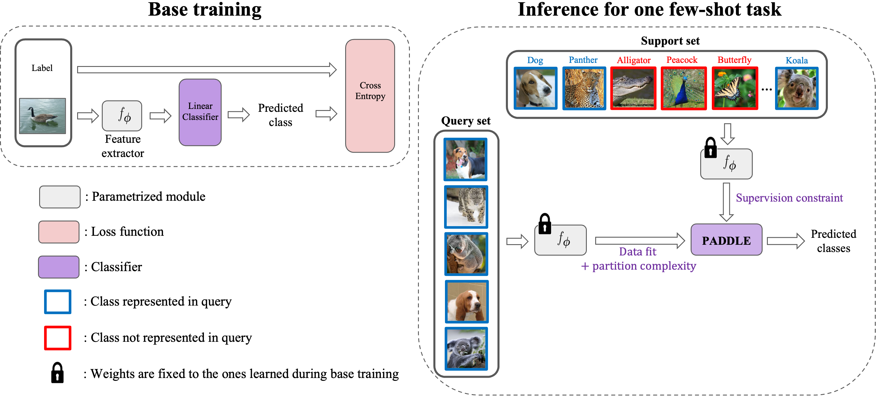
Let $\mathcal{D}_{\text{base}}=\{\bm{x}_{n},\bm{y}_{n}\}_{n=1}^{|\mathcal{D}_{\text{base}}|}$ denotes the base dataset, where each $\bm{x}_{n}\in\mathcal{X}_{\text{base}}$ is a sample from some input space $\mathcal{X}$, $\bm{y}_{n}\in\{0,1\}^{|\mathcal{Y}_{\text{base}}|}$ the associated ground-truth label, and $\mathcal{Y}_{\text{base}}$ the set of base classes. Base training learns a feature extractor $f_{\bm{\phi}}:\mathcal{X}\rightarrow\mathcal{Z}$, with parameters $\bm{\phi}$ and $\mathcal{Z}$ a lower-dimensional space. For this stage, an abundant few-shot literature adopts episodic training, which views $\mathcal{D}_{\text{base}}$ as a series of tasks (or episodes) so as to simulate testing time. Then, a meta-learner is devised to produce the predictions. However, it has been widely established over recent years that a basic training, followed by transfer-learning strategies, outperforms most meta-learning methods [24, 25, 26, 4, 11]. Hence, we adopt a standard cross-entropy training in this work.

Evaluation is carried out over few-shot tasks, each containing samples from $\mathcal{D}_{\text{test}}=\{\bm{x}_{n},\bm{y}_{n}\}_{n=1}^{|\mathcal{D}_{\text{test}}|}$, where $\bm{y}_{n}\in\{0,1\}^{|\mathcal{Y}_{\text{test}}|}$, with constraint ${\mathcal{Y}_{\text{base}}\cap\mathcal{Y}_{\text{test}}=\varnothing}$, i.e., the test and base classes are distinct. Each task includes a labelled support set $\mathbb{S}=\{\bm{x}_{n},\bm{y}_{n}\}_{n\in\mathbbm{I}_{\mathbb{S}}}$ and an unlabelled query set $\mathbb{Q}=\{\bm{x}_{n}\}_{n\in\mathbbm{I}_{\mathbb{Q}}}$, both containing examples from classes in $\mathcal{Y}_{\text{test}}$. Using the feature extractor $f_{\bm{\phi}}$ trained on base data, the goal is to predict the classes of the unlabeled samples in $\mathbb{Q}$ for each few-shot task, independently of the other tasks.

For a given task, let $K~$denote the total number of possible classes that are represented in the labeled support set $\mathbb{S}$, and $K_{\text{eff}}$ the number of classes that appear effectively in unlabeled query set $\mathbb{Q}$ (i.e. classes represented by at least one sample). The standard task generation protocol assumes that the set of effective classes in $\mathbb{Q}$ matches exactly the set of classes in $\mathbb{S}$, i.e. $K~$$=K_{\text{eff}}\ll|\mathcal{Y}_{\text{test}}|$, which amounts to knowing exactly the few classes that appear in the test samples. Then, a fixed number of instances per class are sampled for each query set, forcing class balance. We relax these assumptions, and propose a setting where the set of effective classes in $\mathbb{Q}$ is not known exactly and belongs to a much larger set of possible classes. First, we allow the total number of possible classes $K~$to be higher than typical values, with $K=|\mathcal{Y}_{\text{test}}|$, while keeping the number of effective classes in the query set to be typically much smaller: $K_{\text{eff}}\ll|\mathcal{Y}_{\text{test}}|=K$. For instance, in our experiments, $K~$can go up to $227$. This, as expected, results in $K$-way problems that are more challenging than the standard 5-way tasks used in the few-shot literature. Secondly, once the effective classes are fixed, and given a budget of images, we sample the query set under the data joint distribution (i.e. uniform draws among all available examples), so that the statistics of the sampled query sets more faithfully reflect the natural distribution of classes. Figure 1 illustrates our framework (base training, inference and task generation).

The purpose of objective (2) is to classify the data of a few-shot task with as few unique labels as necessary. The data-fitting term has the same form as the standard $K$-means objective for clustering, but is constrained with supervision from the support-set labels. This term evaluates, within each class $k$, the deviation of features from class prototype $\bm{w}_{k}$, thereby encouraging consistency of samples of the same class. The partition-complexity term implicitly penalizes the number of effective (non-empty) classes that appear in the solution ($K_{\text{eff}}~$$\leq$ $K~$), encouraging low cardinality partitions of query set $\mathbb{Q}$. This term is the Shannon entropy of class proportions within $\mathbb{Q}$: it reaches its minimum when all the samples of $\mathbb{Q}$ belong to a single class, i.e., $\exists j\in\{1,\dots,K\}$ such that $\hat{u}_{j}=1$ and all other proportions vanish. It achieves its maximum for perfectly balanced partitions of $\mathbb{Q}$, satisfying $\hat{u}_{k}=1/K$ for all $k$. In practice, this terms promotes solutions that contain only a handful of effective classes among a larger set of $K$ possible classes.

The objective in (2) could be viewed as a partially-supervised instantiation of the general MDL principle. Originated in information theory, MDL is widely used in statistical model selection [27]. Assume that we want to describe some input data $\bm{Z}=(\bm{z}_{n})_{1\leq n\leq|\mathbb{Q}|}$ with a statistical model $\bm{M}$, among a family of possible models. MDL prescribes that the best model corresponds to the shortest description of the data, according to some coding scheme underlying the model. It balances data-fitting accuracy and model complexity by minimizing ${\cal L}(\bm{Z}|\bm{M})+\lambda{\cal L}(\bm{M})$ w.r.t $\bm{M}$. ${\cal L}(\bm{Z}|\bm{M})$ measures the code length of the prediction of $\bm{Z}$ made by $\bm{M}$, while ${\cal L}(\bm{M})$ encourages simpler models (Occam’s razor [27]), e.g., models with less parameters. For instance, in unsupervised clustering, it is common to minimize a discrete label cost as a measure of model complexity [28, 29, 30]. Such a label cost is the number of effective (non-empty) clusters in the solution, and is used in conjunction with a log-likelihood term for data-fitting:

In this expression, $\bm{M}=\{(\bm{w}_{k})_{1\leq k\leq K},\bm{U}\}$ with $\bm{w}_{k}$ being the parameters of some probability distribution $\mbox{Pr}(\bm{z}_{n}|k;\bm{w}_{k})$ describing the samples in cluster $k$, while $\bm{U}$ contains assignments as denoted above.

The discrete model complexity in (3) is commonly used in MDL-based clustering [28, 29, 30], despite the ensuing optimization difficulty. As this measure is a discrete count of non-empty clusters, it does not accommodate fast optimization techniques. Typically, it is either handled via cluster merging heuristics (starting from an initial set of clusters) [30] or via combinatorial move-making algorithms [28], both of which are computationally intensive, more so when dealing with large sets of classes.

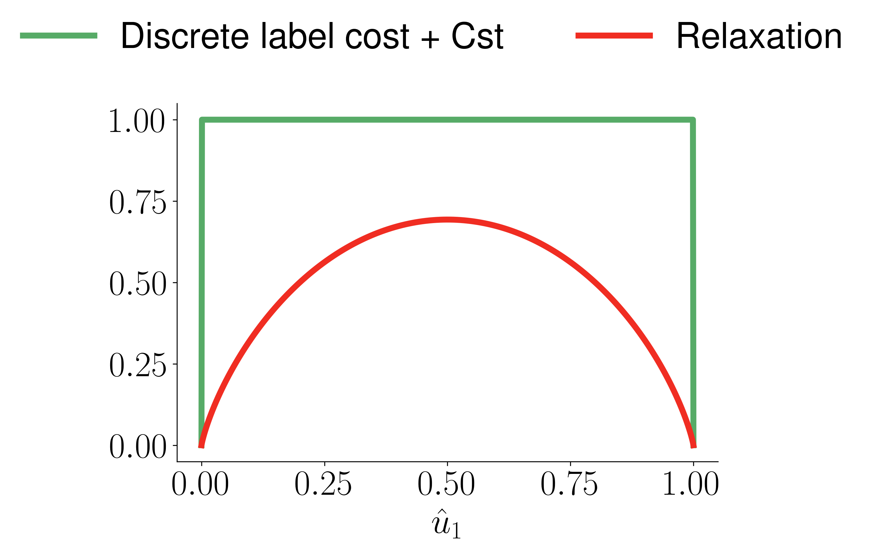
Our partition-complexity term in (2) can be viewed as a continuous relaxation of the discrete label count in (3) (in the supplemental material, we provide a graphical illustration in the case when $K=2$). While penalizing similarly the number of effective classes, it has several advantages over the label count in (3), despite the surprising fact that it is not common in the MDL-based clustering literature, to our best knowledge. First, it is a continuous function of assignment variables $\bm{U}$. This enables us to derive a fast primal-dual block coordinate descent algorithm (Section 4), with convergence guarantee, and a linear computational complexity at each iteration thanks to closed-form updates of the variables. Second, it has a clear MDL interpretation: it measures the number of bits required to encode the set of classes, given class probabilities $\mbox{Pr}(k)=\hat{u}_{k}$, $\forall k\in\{1,\dots,K\}$.

Following the Kraft-McMillan theorem [27], any probability distribution $\mbox{Pr}(\bm{z}_{n}|k;\bm{w}_{k})$ corresponds to some coding scheme for storing the features of cluster $k$, and $-\ln\mbox{Pr}(\bm{z}_{n}|k;\bm{w}_{k})$ is the number of bits required to represent any feature using coding scheme $\mbox{Pr}(\bm{z}_{n}|k;\bm{w}_{k})$. Clearly, our data-fitting term in (2) also fits into this MDL interpretation by assuming that each probability $\mbox{Pr}(\bm{z}_{n}|k;\bm{w}_{k})$ is a Gaussian distribution with mean $\bm{w}_{k}$ and covariance fixed to the identity matrix:

Unlike most of the existing transductive few-shot methods, our MDL formulation does not encode strong assumptions on the label statistics of the query set (e.g. class balance or/and a perfect match between the query and support classes). Information maximization methods, such as [10, 11], maximise the confidence of the sample-wise predictions while encouraging class balance. Optimal transport methods [6, 7] estimate an optimal mapping matrix, which could be viewed as a joint probability distribution over the features and the labels, while imposing a hard class-balance constraint via the Sinkhorn-Knopp algorithm. Both information-maximization and optimal-transport methods have inherent class-balance bias and, as shown in the experiments, undergo a drastic drop in accuracy when the number of possible classes increases (as this corresponds to highly imbalanced problems). Prototype rectification [8] transforms the query features so as to minimize the difference between the overall statistics of the query and support sets. This relies on the assumption that the support and query classes match perfectly. Therefore, it is not adapted to our setting. Inspired from graphical models, the Laplacian regularization in [4] is a pairwise label correction (rather than a learning) method, which encourages assigning the same label to query samples that are close in the input space; it does not learn a class representation from the query set (the prototypes being fixed as those of the support set).

Another interesting view of our few-shot inference objective in (2) can be drawn from the probabilistic $K$-means objective²² 2 In the general context of clustering, the name probabilistic $K$-means was first coined by [31]., well-known in the clustering literature [31, 32, 33]. In fact, probabilistic $K$-means corresponds to minimizing ${\cal L}(\bm{Z}|\bm{M})$ in (4) as a generalization of $K$-means, which corresponds to the particular Gaussian choice in (5). It is a well-known that probabilistic $K$-means has a strong bias towards balanced partitions [31, 33]. The objective can be decomposed to reveal a hidden term promoting class balance. Using Bayes rule $\mbox{Pr}(k|\bm{z}_{n};\bm{w}_{k})\propto\mbox{Pr}(\bm{z}_{n}|k;\bm{w}_{k})\mbox{Pr}(k)$, empirical estimates of marginal class probabilities $\mbox{Pr}(k)=\hat{u}_{k}$, and the choice of $\mbox{Pr}(\bm{z}_{n}|k;\bm{w}_{k})$ in (5), we have:

where $\stackrel{{\scriptstyle\mathclap{\mbox{c}}}}{{=}}$ stands for equality, up to an additive constant independent of optimization variables. Minimizing the last term in the second line of (6) has an effect opposite to the model-complexity term in our objective in (2): it reaches its minimum for perfectly balanced partitions. Therefore, our objective in (2) is a way to mitigate such a bias in $K$-means, allowing imbalanced partitions. This suggests setting $\lambda=|\mathbb{Q}|$ to compensate for the hidden class-balance term in $K$-means. This would make our inference hyper-parameter free. Thus, for our study, we fixed $\lambda=|\mathbb{Q}|$ in all benchmarks, without optimizing the parameter $\lambda$ via validation.

We transform problem (2) into an equivalent optimization problem by introducing a dual variable. Let us first define the linear operator $\bm{A}\colon(\mathbb{R}^{K})^{N}\longrightarrow\mathbb{R}^{K}$, which maps the probabilities to the proportions of the classes, i.e. $\bm{A}:\bm{U}\mapsto(\hat{u}_{k})_{1\leq k\leq K}$. Then, problem (2) can be re-written as follows:

where $H$ is the negative entropy function on the positive orthant of $\mathbb{R}^{K}$: $H(\bm{x})=\sum_{k=1}^{K}\varphi(x_{k})$ for $\bm{x}=(x_{k})_{1\leq k\leq K}\in\mathbb{R}^{K}$, with

We can now appeal to the concept of Fenchel-Legendre conjugate function. For a given convex function $f$, its conjugate function, denoted by $f^{*}$, is defined as $f^{*}(\bm{V})=\displaystyle\sup_{\bm{U}}(\langle\bm{V},\bm{U}\rangle-f(\bm{U}))$, where $\bm{V}$ is a dual variable [34, Def. 13.1] and $\langle\cdot,\cdot\rangle$ denotes the Euclidean scalar product on $\mathbb{R}^{K\times N}$. Since function $H$ is a proper, lower semicontinuous, convex function, according to the Fenchel-Moreau theorem [34, Thm. 13.37], the equality $H=(H^{*})^{*}$ holds. Hence, it follows that

Plugging (8) into (4), and using the expression of $H^{*}$ [35, Ex. 3.21], one obtains the following minimization problem with respect to the primal variable $\bm{U}$, the weights $\bm{W}$ and the dual variable $\bm{V}$:

To deal efficiently with the simplex constraint in (9), we add an entropic barrier on soft assignment variables $\bm{u}_{n}$, leading to the following modified problem:

The last term in (10) acts as a barrier for imposing constraints $\bm{u}_{n}\geq 0$ and, at each iteration, yields closed-form updates of both the dual variables for constraints $\sum_{k=1}^{K}u_{n,k}=1$ and assignments $\bm{U}$. This simplifies the iterative constrained-minimization steps over $\bm{U}$ in our algorithm below through simple closed-form softmax operations (derivation details provided in supplemental material).

To minimize the cost function in (10), we pursue a block coordinate descent approach [36, 37], which is guaranteed to converge; see Proposition 1 below. At each iteration, we successively minimize the objective with respect to the variables $\bm{U}$, $\bm{V}$, and $\bm{W}$ respectively. To do so, we use the adjoint operator of $\bm{A}$, which we denote $\bm{A}^{*}$. Our algorithm is detailed in Algorithm 1.

In addition to its practical advantages in terms of implementation, our algorithm benefits from the convergence guarantee described in Proposition 1.

A detailed proof of Proposition 1 is provided in the supplementary material.

References

- [1] J. Snell, K. Swersky, and R. Zemel, “Prototypical networks for few-shot learning,” in Neural Information Processing Systems (NeurIPS), 2017.
- [2] C. Finn, P. Abbeel, and S. Levine, “Model-agnostic meta-learning for fast adaptation of deep networks,” in International Conference on Machine Learning (ICML), 2017.
- [3] O. Vinyals, C. Blundell, T. P. Lillicrap, K. Kavukcuoglu, and D. Wierstra, “Matching networks for one shot learning,” in Neural Information Processing Systems (NeurIPS), 2016.
- [4] I. M. Ziko, J. Dolz, E. Granger, and I. Ben Ayed, “Laplacian regularized few-shot learning,” in International Conference on Machine Learning (ICML), 2020.
- [5] L. Yanbin, J. Lee, M. Park, S. Kim, E. Yang, S. Hwang, and Y. Yang, “Learning to propagate labels: Transductive propagation network for few-shot learning,” in International Conference on Learning Representations (ICLR), 2019.
- [6] M. Lazarou, T. Stathaki, and Y. Avrithis, “Iterative label cleaning for transductive and semi-supervised few-shot learning,” in IEEE/CVF Conference on Computer Vision (ICCV), 2021.
- [7] Y. Hu, V. Gripon, and S. Pateux, “Leveraging the feature distribution in transfer-based few-shot learning,” in International Conference on Artificial Neural Networks (ICANN), 2021.
- [8] J. Liu, L. Song, and Y. Qin, “Prototype rectification for few-shot learning,” in European Conference on Computer Vision (ECCV), 2020.
- [9] W. Cui and Y. Guo, “Parameterless transductive feature re-representation for few-shot learning,” in International Conference on Machine Learning (ICML), 2021.
- [10] O. Veilleux, M. Boudiaf, P. Piantanida, and I. Ben Ayed, “Realistic evaluation of transductive few-shot learning,” Neural Information Processing Systems (NeurIPS), 2021.
- [11] M. Boudiaf, I. M. Ziko, J. Rony, J. Dolz, P. Piantanida, and I. Ben Ayed, “Transductive information maximization for few-shot learning,” in Neural Information Processing Systems (NeurIPS), 2020.
- [12] M. Boudiaf, H. Kervadec, I. M. Ziko, P. Piantanida, I. B. Ayed, and J. Dolz, “Few-shot segmentation without meta-learning: A good transductive inference is all you need?” in IEEE/CVF Conference on Computer Vision and Pattern Recognition (CVPR), 2021.
- [13] J. Bronskill, J. Gordon, J. Requeima, S. Nowozin, and R. E. Turner, “Tasknorm: Rethinking batch normalization for meta-learning,” in International Conference on Machine Learning (ICML), 2020.
- [14] G. S. Dhillon, P. Chaudhari, A. Ravichandran, and S. Soatto, “A baseline for few-shot image classification,” in International Conference on Learning Representations (ICLR), 2020.
- [15] Y. Wang, C. Xu, C. Liu, L. Zhang, and Y. Fu, “Instance credibility inference for few-shot learning,” in IEEE/CVF Conference on Computer Vision and Pattern Recognition (CVPR), 2020.
- [16] G. Qi, H. Yu, Z. Lu, and S. Li, “Transductive few-shot classification on the oblique manifold,” in Proceedings of the IEEE/CVF International Conference on Computer Vision, 2021, pp. 8412–8422.
- [17] X. Shen, Y. Xiao, S. X. Hu, O. Sbai, and M. Aubry, “Re-ranking for image retrieval and transductive few-shot classification,” in Neural Information Processing Systems (NeurIPS), 2021.
- [18] M. Ren, E. Triantafillou, S. Ravi, J. Snell, K. Swersky, J. B. Tenenbaum, H. Larochelle, and R. S. Zemel, “Meta-learning for semi-supervised few-shot classification,” in International Conference on Learning Representations (ICLR), 2018.
- [19] V. N. Vapnik, “An overview of statistical learning theory,” IEEE Transactions on Neural Networks (TNN), vol. 10, no. 5, pp. 988–999, 1999.
- [20] T. Joachims, “Transductive inference for text classification using support vector machines,” in International Conference on Machine Learning (ICML), 1999.
- [21] Z. Dengyong, O. Bousquet, T. N. Lal, J. Weston, and B. Schölkopf, “Learning with local and global consistency,” in Neural Information Processing Systems (NeurIPS), 2004.
- [22] M. Lichtenstein, P. Sattigeri, R. Feris, R. Giryes, and L. Karlinsky, “TAFSSL: Task-adaptive feature sub-space learning for few-shot classification,” in European Conference on Computer Vision. Springer, 2020, pp. 522–539.
- [23] D. Wertheimer and B. Hariharan, “Few-shot learning with localization in realistic settings,” in Proceedings of the IEEE Conference on Computer Vision and Pattern Recognition, 2019, pp. 6558–6567.
- [24] W.-Y. Chen, Y.-C. Liu, Z. Kira, Y.-C. F. Wang, and J.-B. Huang, “A closer look at few-shot classification,” in International Conference on Learning Representations (ICLR), 2019.
- [25] Y. Wang, W.-L. Chao, K. Q. Weinberger, and L. van der Maaten, “Simpleshot: Revisiting nearest-neighbor classification for few-shot learning,” arXiv preprint:1911.04623, 2019.
- [26] Y. Tian, Y. Wang, D. Krishnan, J. B. Tenenbaum, and P. Isola, “Rethinking few-shot image classification: a good embedding is all you need?” in European Conference on Computer Vision (ECCV), 2020.
- [27] D. J. C. MacKay, Information Theory, Inference, and Learning Algorithms. Cambridge University Press, 2003.
- [28] A. Delong, A. Osokin, H. N. Isack, and Y. Boykov, “Fast approximate energy minimization with label costs,” International Journal of Computer Vision, vol. 96, no. 1, pp. 1–27, 2012.
- [29] J. Yuan and Y. Boykov, “Tv-based multi-label image segmentation with label cost prior,” in British Machine Vision Conference (BMVC), 2010.
- [30] S. C. Zhu and A. L. Yuille, “Region competition: unifying snakes, region growing, and bayes/mdl for multiband image segmentation,” IEEE Trans. on Pattern Analysis and Machine Intelligence (TPAMI), vol. 18, no. 9, pp. 884–900, 1996.
- [31] M. Kearns, Y. Mansour, and A. Ng, “An information-theoretic analysis of hard and soft assignment methods for clustering,” in Conference on Uncertainty in Artificial Intelligence (UAI), 1997.
- [32] M. Tang, D. Marin, I. Ben Ayed, and Y. Boykov, “Kernel cuts: Kernel and spectral clustering meet regularization,” International Journal of Computer Vision, vol. 127, no. 5, pp. 477–511, 2019.
- [33] Y. Boykov, H. N. Isack, C. Olsson, and I. Ben Ayed, “Volumetric bias in segmentation and reconstruction: Secrets and solutions,” in IEEE/CVF International Conference on Computer Vision (ICCV), 2005.
- [34] H. H. Bauschke, P. L. Combettes et al., Convex Analysis and Monotone Operator Theory in Hilbert Spaces. Springer, 2011, vol. 408.
- [35] S. Boyd, N. Parikh, and E. Chu, Distributed Optimization and Statistical Learning via the Alternating Direction Method of Multipliers. Now Publishers Inc, 2011.
- [36] D. Bertsekas, Nonlinear Programming, ser. Athena Scientific optimization and computation series. Athena Scientific, 1995.
- [37] Y. Xu and W. Yin, “A block coordinate descent method for regularized multiconvex optimization with applications to nonnegative tensor factorization and completion,” SIAM Journal on Imaging Sciences, vol. 6, no. 3, pp. 1758–1789, 2013.
- [38] O. Russakovsky, J. Deng, H. Su, J. Krause, S. Satheesh, S. Ma, Z. Huang, A. Karpathy, A. Khosla, M. Bernstein, A. C. Berg, and L. Fei-Fei, “ImageNet Large Scale Visual Recognition Challenge,” International Journal of Computer Vision (IJCV), vol. 115, no. 3, pp. 211–252, 2015.
- [39] S. Ravi and H. Larochelle, “Optimization as a model for few-shot learning,” in International Conference on Learning Representations (ICLR), 2017.
- [40] C. Bauckhage, “NumPy/SciPy recipes for data science: Projections onto the standard simplex,” University of Bonn, Tech. Rep., 2020.
- [41] D. P. Kingma and J. Ba, “Adam: A method for stochastic optimization,” arXiv preprint arXiv:1412.6980, 2014.
- [42] Y. Guo, N. Codella, L. Karlinsky, J. V. Codella, J. R. Smith, K. Saenko, T. Rosing, and R. Feris, “A broader study of cross-domain few-shot learning,” in European Conference Computer Vision (ECCV), 2020.
- [43] E. Bennequin, V. Bouvier, M. Tami, A. Toubhans, and C. Hudelot, “Bridging few-shot learning and adaptation: New challenges of support-query shift,” in Joint European Conference on Machine Learning and Knowledge Discovery in Databases, 2021.
- [44] P. L. Combettes and J.-C. Pesquet, “Deep neural network structures solving variational inequalities,” Set-Valued and Variational Analysis, vol. 28, no. 3, pp. 491–518, 2020.
- [45] P. Tseng, “Convergence of a block coordinate descent method for nondifferentiable minimization,” Journal of optimization theory and applications, vol. 109, no. 3, pp. 475–494, 2001.