Parameter-free Regret in High Probability with Heavy Tails

In this paper, we consider the problem of online learning with convex losses, also called online convex optimization, with heavy-tailed stochastic subgradients. In the classical online convex optimization setting, given a convex set $\mathcal{W}$, a learning algorithm must repeatedly output a vector $\mathbf{w}_{t}\in\mathcal{W}$, and then observe a convex loss function $\ell_{t}:\mathcal{W}\to\mathbb{R}$ and incur a loss of $\ell_{t}(\mathbf{w}_{t})$. After $T$ such rounds, the algorithm’s quality is measured by the regret with respect to a fixed competitor $\mathbf{u}\in\mathcal{W}$:

Online convex optimization is widely applicable, and has been used to design popular stochastic optimization algorithms ((Duchi et al. 2010a; Kingma and Ba 2014; Reddi et al. 2018)), for control of linear dynamical systems (Agarwal et al. 2019), or even building concentration inequalities (Vovk 2007; Waudby-Smith and Ramdas 2020; Orabona and Jun 2021).

A popular approach to this problem reduces it to online linear optimization (OLO): if $\mathbf{g}_{t}$ is a subgradient of $\ell_{t}$ at $\mathbf{w}_{t}$, then $R_{T}(\mathbf{u})\leq\sum_{t=1}^{T}\langle\mathbf{g}_{t},\mathbf{w}_{t}-\mathbf{u}\rangle$ so that it suffices to design an algorithm that considers only linear losses $\mathbf{w}\mapsto\langle\mathbf{g}_{t},\mathbf{w}\rangle$. Then, by assuming that the domain $\mathcal{W}$ has some finite diameter $D$, standard arguments show that online gradient descent (Zinkevich 2003) and its variants achieve $R_{T}(\mathbf{u})\leq O(D\sqrt{T})$ for all $\mathbf{u}\in\mathcal{W}$. See the excellent books Cesa-Bianchi and Lugosi 2006; Shalev-Shwartz 2011; Hazan 2019; Orabona 2019 for more detail.

Deviating from the classical setting, we study the more difficult case in which, (1) the domain $\mathcal{W}$ may have infinite diameter (such as $\mathcal{W}=\mathbb{R}^{d}$), and (2) instead of observing the loss $\ell_{t}$, the algorithm is presented only with a potentially heavy-tailed stochastic subgradient estimate $\mathbf{g}_{t}$ with $\mathop{\mathbb{E}}[\mathbf{g}_{t}|\mathbf{w}_{t}]\in\partial\ell_{t}(\mathbf{w}_{t})$. Our goal is to develop algorithms that, with high probability, obtain essentially the same regret bound that would be achievable even if the full information was available.

Considering only the setting of infinite diameter $\mathcal{W}$ with exact subgradients $\mathbf{g}_{t}\in\partial\ell_{t}(\mathbf{w}_{t})$, past work has achieved bounds of the form $R_{T}(\mathbf{u})\leq\tilde{O}(\epsilon+\|\mathbf{u}\|\sqrt{T})$ for all $\mathbf{u}\in\mathcal{W}$ simultaneously for any user-specified $\epsilon$, directly generalizing the $O(D\sqrt{T})$ rate available when $D<\infty$ (Orabona and Pál 2016; Cutkosky and Orabona 2018; Foster et al. 2017; Mhammedi and Koolen 2020; Chen et al. 2021). As such algorithms do not require knowledge of the norm $\|\mathbf{u}\|$ that is usually used to specify a learning rate for gradient descent, we will call them parameter-free. Note that such algorithms typically guarantee constant $R_{T}(0)$, which is not achieved by any known form of gradient descent.

While parameter-free algorithms appear to fully generalize the finite-diameter case, they fall short when $\mathbf{g}_{t}$ is a stochastic subgradient estimate. In particular, lower-bounds suggest that parameter-free algorithms must require Lipschitz $\ell_{t}$ (Cutkosky and Boahen 2017), which means that care must be taken when using $\mathbf{g}_{t}$ with unbounded noise as this may make $\ell_{t}$ “appear” to be non-Lipschitz. In the case of sub-exponential $\mathbf{g}_{t}$, Jun and Orabona 2019; van der Hoeven 2019 provide parameter-free algorithms that achieve $\mathop{\mathbb{E}}[R_{T}(\mathbf{u})]\leq\tilde{O}(\epsilon+\|\mathbf{u}\|\sqrt{T})$, but these techniques do not easily extend to heavy-tailed $\mathbf{g}_{t}$ or to high-probability bounds. The high-probability statement is particularly elusive (even with sub-exponential $\mathbf{g}_{t}$) because standard martingale concentration approaches appear to fail spectacularly. This failure may be counterintuitive: for finite diameter $\mathcal{W}$, one can observe that $\langle\mathbf{g}_{t}-\mathop{\mathbb{E}}[\mathbf{g}_{t}],\mathbf{w}_{t}-\mathbf{u}\rangle$ forms a martingale difference sequence with variance determined by $\|\mathbf{w}_{t}-\mathbf{u}\|\leq D$, which allows for relatively straightforward high-probability bounds. However, parameter-free algorithms typically exhibit exponentially growing $\|\mathbf{w}_{t}\|$ in order to compete with all possible scales of $\|\mathbf{u}\|$, which appears to stymie such arguments.

Our work overcomes these issues. Requiring only that $\mathbf{g}_{t}$ have a bounded $\mathfrak{p}^{th}$ moment for some $\mathfrak{p}\in(1,2]$, we devise a new algorithm whose regret with probability at least $1-\delta$ is $R_{T}(\mathbf{u})\leq\tilde{O}(\epsilon+\|\mathbf{u}\|T^{1/\mathfrak{p}}\log(1/\delta))$ for all $\mathbf{u}$ simultaneously. The $T^{1/\mathfrak{p}}$ dependency is unimprovable Bubeck et al. 2013; Vural et al. 2022. Moreover, we achieve these results simply by adding novel and carefully designed regularizers to the losses $\ell_{t}$ in a way that converts any parameter-free algorithm with sufficiently small regret into one with the desired high probability guarantee.

Motivation: High-probability analysis is appealing since it provides a confidence guarantee for an algorithm over a single run. This is crucially important in the online setting in which we must make irrevocable decisions. It is also important in the standard stochastic optimization setting encountered throughout machine learning as it ensures that even a single potentially very expensive training run will produce a good result. See Harvey et al. 2019; Li and Orabona 2020; Madden et al. 2020; Kavis et al. 2022 for more discussion on the importance of high-probability bounds in this setting. This goal naturally synergizes with the overall objective of parameter-free algorithms, which attempt to provide the best-tuned performance after a single pass over the data. In addition, we consider the presence of heavy-tailed stochastic gradients, which are empirically observed in large neural network architectures Zhang et al. 2020; Zhou et al. 2020. The online optimization problem we consider is actually fundamentally more difficult than the stochastic optimization problem: indeed Carmon and Hinder 2022 show that lower bounds for parameter-free online optimization to not apply to stochastic optimization, and provide a high-probability analysis for the latter setting. In contrast, the more flexible online setting allows us build more robust algorithms that can perform well in non-stationary or even adversarial environments.

Contribution and Organization: After formally introducing and discussing our setup in Sections 2, we then proceed to conduct an initial analysis for the 1-D case $\mathcal{W}=\mathbb{R}$ in 3. First (Section 4), we introduce a parameter-free algorithm for sub-exponential $g_{t}$ that achieves regret $\tilde{O}(\epsilon+|u|\sqrt{T})$ in high probability. This already improves significantly on prior work, and is accomplished by introducing a novel regularizer that “cancels” some unbounded martingale concentration terms, a technique that may have wider application. Secondly (Section 5), we extend to heavy-tailed $g_{t}$ by employing clipping, which has been used in prior work on optimization (Bubeck et al. 2013; Gorbunov et al. 2020; Zhang et al. 2020; Cutkosky and Mehta 2021) to convert heavy-tailed estimates into sub-exponential ones. This clipping introduces some bias that must be carefully offset by yet another novel regularization (which may again be of independent interest) in order to yield our final $\tilde{O}(\epsilon+|u|T^{1/\mathfrak{p}})$ parameter-free regret guarantee. Finally (Section 6), we extend to arbitrary dimensions via the reduction from Cutkosky and Orabona 2018.

Our algorithms interact with an adversary in which for $t=1\dots T$ the algorithm first outputs a vector $\mathbf{w}_{t}\in\mathcal{W}$ for $\mathcal{W}$ a convex subset of some real Hilbert space, and then the adversary chooses a convex and $G$-Lipschitz loss function $\ell_{t}:\mathcal{W}\to\mathbb{R}$ and a distribution $P_{t}$ such that for $\mathbf{g}_{t}\sim P_{t}$, $\mathop{\mathbb{E}}[\mathbf{g}_{t}]\in\partial\ell_{t}(\mathbf{w}_{t})$ and $\mathop{\mathbb{E}}[\|\mathbf{g}_{t}-\mathop{\mathbb{E}}[\mathbf{g}_{t}]\|^{\mathfrak{p}}]\leq\sigma^{\mathfrak{p}}$ for some $\mathfrak{p}\in(1,2]$. The algorithm then observes a random sample $\mathbf{g}_{t}\sim P_{t}$. After $t$ rounds, we compute the regret, which is a function $R_{t}(\mathbf{u})=\sum_{i=1}^{t}\ell_{i}(\mathbf{w}_{i})-\ell_{i}(\mathbf{u})$. Our goal is to guarantee $R_{T}(\mathbf{u})\leq\epsilon+\tilde{O}(\|\mathbf{u}\|T^{1/\mathfrak{p}})$ for all $\mathbf{u}$ simultaneously with high probability.

Throughout this paper we will employ the notion of a sub-exponential random sequence:

We drop the subscript $t$ when we have uniform (not time-varying) sub-exponential parameters $(\sigma,b)$. We use bold font ($\mathbf{g}_{t}$) to refer to vectors and normal font $(g_{t})$ to refer to scalars. Occasionally, we abuse notation to write $\nabla\ell_{t}(\mathbf{w}_{t})$ for an arbitrary element of $\partial\ell_{t}(\mathbf{w}_{t})$.

We present our results using $O(\cdot)$ to hide constant factors, and $\tilde{O}(\cdot)$ to hide $\log$ factors (such as some power of $\log T$ dependence) in the main text, the exact results are left at the last line of the proof for interested readers.

Finally, observe that by the unconstrained-to-constrained conversion of Cutkosky and Orabona 2018, we need only consider the case that $\mathcal{W}$ is an entire vector space. By solving the problem for this case, the reduction implies a high-probability regret algorithm for any convex $\mathcal{W}$.

A reader experienced with high probability bounds in online optimization may suspect that one could apply fairly standard approaches such as gradient clipping and martingale concentration to easily achieve high probability bounds with heavy tails. While such techniques do appear in our development, the story is far from straightforward. In this section, we will outline these non-intuitive difficulties. For a further discussion, see Section 3 of Jun and Orabona 2019.

For simplicity, consider $w_{t}\in\mathbb{R}$. Before attempting a high probability bound, one may try to derive a regret bound in expectation with heavy-tailed (or even light-tailed) gradient $g_{t}$ via the following calculation:

The second sum from above vanishes, so one is tempted to send $g_{t}$ directly to some existing parameter-free algorithm to obtain low regret. Unfortunately, most parameter-free algorithms require a uniform bound on $|g_{t}|$ - even a single bound-violating $g_{t}$ could be catastrophic (Cutkosky and Boahen 2017). With heavy-tailed $g_{t}$, we are quite likely to encounter such a bound-violating $g_{t}$ for any reasonable uniform bound. In fact, the issue is difficult even for light-tailed $g_{t}$, as described in detail by Jun and Orabona 2019.

A natural approach to overcome this uniform bound issue is to incorporate some form of clipping, a commonly used technique controlling for heavy-tailed subgradients. The clipped subgradient $\hat{g}_{t}$ is defined below with a positive clipping parameter $\tau$ as:

If we run algorithms on uniformly bounded $\hat{g}_{t}$ instead, the expected regret can now be written as:

Since $|\hat{g}_{t}|\leq\tau$, the first term can in fact be controlled for appropriate $\tau$ at a rate of $\tilde{O}(\epsilon+|u|\sqrt{T})$ using sufficiently advanced parameter-free algorithms (e.g. Cutkosky and Orabona 2018). However, now bias accumulates in the last term, which is difficult to bound due to the dependency on $w_{t}$. On the surface, understanding this dependency appears to require detailed (and difficult) analysis of the dynamics of the parameter-free algorithm. In fact, from naive inspection of the updates for standard parameter-free algorithms, one expects that $|w_{t}|$ could actually grow exponentially fast in $t$, leading to a very large bias term.

Finally, disregarding these challenges faced even in expectation, to derive a high-probability bound the natural approach is to bound the middle sum in (1) via some martingale concentration argument. Unfortunately, the variance process for this martingale depends on $w_{t}$ just like the bias term. In fact, this issue appears even if the original $g_{t}$ already have bounded norm, which is the most extreme version of light tails! Thus, we again appear to encounter a need for small $w_{t}$, which may instead grow exponentially. In summary, the unbounded nature of $w_{t}$ makes dealing with any kind of stochasticity in the $g_{t}$ very difficult. In this work we will develop techniques based on regularization that intuitively force the $w_{t}$ to behave well, eventually enabling our high-probability regret bounds.

In this section, we describe how to obtain regret bound in high probability for stochastic subgradients $g_{t}$ for which $\mathop{\mathbb{E}}[g_{t}^{2}]\leq\sigma^{2}$ and $|g_{t}|\leq b$ for some $\sigma$ and $b$ (in particular, $g_{t}$ exhibits $(\sigma,4b)$ sub-exponential noise). We focus on the 1-dimensional case with $\mathcal{W}=\mathbb{R}$. The extension to more general $\mathcal{W}$ is covered in Section 6. Our method involves two coordinated techniques. First, we introduce a carefully designed regularizer $\psi_{t}$ such that any algorithm that achieves low regret with respect to the losses $w\mapsto g_{t}w+\psi_{t}(w)$ will automatically ensure low regret with high probability on the original losses $\ell_{t}$. Unfortunately, $\psi_{t}$ is not Lipschitz and so it is still not obvious how to obtain low regret. We overcome this final issue by an “implicit” modification of the optimistic parameter-free algorithm of Cutkosky 2019. Our overall goal is a regret bound of $R_{T}(u)\leq\tilde{O}(\epsilon+|u|(\sigma+G)\sqrt{T}+b|u|)$ for all $u$ with high probability. Note that with this bound, $b$ can be $O(\sqrt{T})$ before it becomes a significant factor in the regret.

Let us proceed to sketch the first (and most critical) part of this procedure: Define $\epsilon_{t}=\nabla\ell_{t}(w_{t})-g_{t}$, so that $\epsilon_{t}$ captures the “noise” in the gradient estimate $g_{t}$. In this section, we assume that $\epsilon_{t}$ is $(\sigma,4b)$ sub-exponential for all $t$ for some given $\sigma,b$ and $|g_{t}|\leq b$. Then we can write:

Now, the natural strategy is to run an OLO algorithm $\mathcal{A}$ on the observed $g_{t}$, which will obtain some regret $R^{\mathcal{A}}_{T}(u)=\sum_{t=1}^{T}\langle g_{t},w_{t}-u\rangle$, and then show that the remaining Noise terms are small. To this end, from sub-exponential martingale concentration, we might hope to show that with probability $1-\delta$, we have an identity similar to:

The dependency of $|u|$ above appears to be relatively innocuous as it only contributes $\tilde{O}(|u|\sigma\sqrt{T}+|u|b)$ to the regret. The $w_{t}$-dependent term is more difficult as it involves a dependency on the algorithm $\mathcal{A}$. This captures the complexity of our unbounded setting: in a bounded domain, the situation is far simpler as we can uniformly bound $|w_{t}|\leq D$, ideally leaving us with an $\tilde{O}(D\sqrt{T})$ bound overall.

Unfortunately, in the unconstrained case, $|w_{t}|$ could grow exponentially ($|w_{t}|\sim 2^{t})$ even when $u$ is very small, so we cannot rely on a uniform bound. In fact, even in the finite-diameter case, if we wish to guarantee $R_{T}(0)\leq\epsilon$, the bound $|w_{t}|\leq D$ is still too coarse. The resolution is to instead feed the algorithm $\mathcal{A}$ a regularized loss $\hat{\ell}_{t}(w)=\langle g_{t},w\rangle+\psi_{t}(w)$, where $\psi_{t}$ will “cancel” the $w_{t}$ dependency in the martingale concentration. That is, we now define $R^{\mathcal{A}}_{T}(u)=\sum_{t=1}^{T}\hat{\ell}_{t}(w_{t})-\hat{\ell}_{t}(u)$ and rearrange:

And now combine equations (2) and (3):

From this, we can read off the desired properties of $\psi_{t}$: (1) $\psi_{t}$ should be large enough that $\sum_{t=1}^{T}\psi_{t}(w_{t})\geq\sigma\sqrt{\sum_{t=1}^{T}w_{t}^{2}\log(1/\delta)}+b\max_{t}|w_{t}|\log(1/\delta)$, (2) $\psi_{t}$ should be small enough that $\sum_{t=1}^{T}\psi_{t}(u)\leq\tilde{O}(|u|\sqrt{T})$, and (3) $\psi_{t}$ should be such that $R_{T}^{\mathcal{A}}(u)=\tilde{O}(\epsilon+|u|\sqrt{T})$ for an appropriate algorithm $\mathcal{A}$. If we can exhibit a $\psi_{t}$ satisfying all three properties, we will have developed a regret bound of $\tilde{O}(\epsilon+|u|\sqrt{T})$ in high probability.

It turns out that the modified Huber loss $r_{t}(w)$ defined in equation (5) and (6) with appropriately chosen constants $c_{1},c_{2},p_{1},p_{2},\alpha_{1},\alpha_{2}$ satisfies criterion (1) and (2).

Let us take a moment to gain some intuition for these functions $r_{t}$ and $\psi_{t}$. First, observe that $r_{t}$ is always continuously differentiable, and that $r_{t}$’s definition requires knowledge of $w_{t}$. This is acceptable because online learning algorithms must be able to handle even adaptively chosen losses. In particular, consider the $p=2$ case, $r_{t}(w;c,2,\alpha)$ for some positive constants $c$ and $\alpha$. We plot this function in Figure 1, where one can see that $r_{t}$ grows quadratically for $|w|\leq|w_{t}|$, but grows only linearly afterwards so that $r_{t}$ is Lipschitz.

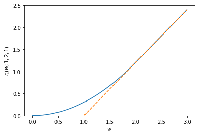
Eventually, in Lemma 13 we will show that this functions satisfies

so that for appropriate choice of $c$ and $\alpha$, $r_{t}(w;c,2,\alpha)$ will cancel the $O(\sqrt{\sum_{t=1}^{T}w_{t}^{2}})$ martingale concentration term while not adding too much to the regret - it satisfies criteria (1) and (2). The lower-bound follows from the standard inequality $\sqrt{a+b}\leq\sqrt{a}+\frac{b}{\sqrt{a+b}}$ since $r_{t}(w_{t})=c\frac{w_{t}^{2}}{\sqrt{\alpha^{2}+\sum_{i=1}^{t}w_{i}^{2}}}$. The upper-bound is more subtle, and involves the piece-wise definition. For simplicity, suppose it were true that either $|w_{t}|<|u|$ for all $t$ or $|w_{t}|\geq|u|$ for all $t$. In the former case, $\sum_{t=1}^{T}r_{t}(u)=O\left(|u|\sum_{t=1}^{T}\frac{|w_{t}|}{\sqrt{\alpha+\sum_{i=1}^{t}w_{i}^{2}}}\right)$, which via algebraic manipulation can be bounded as $\tilde{O}(|u|\sqrt{T})$. In the latter case, we have $\sum_{t=1}^{T}\frac{|u|^{2}}{\sqrt{\alpha^{2}+\sum_{i=1}^{t}w_{t}^{2}}}\leq\sum_{t=1}^{T}\frac{|u|^{2}}{\sqrt{\alpha^{2}+tu^{2}}}=\tilde{O}(|u|\sqrt{T})$ so that both cases result in the desired bound on $\sum_{t=1}^{T}r_{t}(u)$. The general setting is handled by partitioning the sum into two sets depending on whether $|w_{t}|\leq|u|$. In order to cancel the $\max_{t}|w_{t}|$ term in the martingale concentration, we employ $p=\log T$. This choice is motivated by the observation that $\|\mathbf{v}\|_{\log T}\in[\|\mathbf{v}\|_{\infty},\exp(1)\|\mathbf{v}\|_{\infty}]$ for all $\mathbf{v}\in\mathbb{R}^{\log T}$. With this identity in hand, the argument is very similar to the $p=2$ case.

The correct values for the constants are provided in Theorem 3. Again, at a high level, the important constants are $p_{1}$ and $p_{2}$. With $p_{1}=2$, we allow $\sum_{t}r_{t}(w_{t};p=2)$ to cancel out the $\sqrt{\sum_{t}w_{t}^{2}}$ martingale concentration term, while with $p_{2}=\log T$, $\sum_{t}r_{t}(w_{t};p=\log T)$ cancels that $\max_{t}|w_{t}|$ term.

It remains to show that $\psi_{t}$ also allows for small $R_{T}^{\mathcal{A}}(u)$ and so satisfies criterion (3). Unfortunately, our setting for $c_{2}$ in the definition of $\psi_{t}$ is $\tilde{O}(b)$, which means that $\psi_{t}$ is $\tilde{O}(b)$-Lipschitz. Since we wish to allow for $b=\Theta(\sqrt{T})$, this means that we cannot simply let $\mathcal{A}$ linearize $\psi_{t}$ and apply an arbitrary OLO algorithm. Instead, we must exploit the fact that $\psi_{t}$ is known before $g_{t}$ is revealed. That is, algorithm $\mathcal{A}$ is chosen to exploit the structure composite loss $\hat{\ell}_{t}(w)$. Intuitively, the regret of a composite loss should depend only on the non-composite $g_{t}$ terms (as in e.g. Duchi et al. 2010b). Our situation is slightly more complicated as $\psi_{t}$ depends on $w_{t}$ as well, but we nevertheless achieve the desired result via a modification of the parameter-free optimistic reduction in Cutkosky 2019. For technical reasons, this algorithm still requires $|g_{t}|\leq b$ with probability 1, but obtains regret only $R^{\mathcal{A}}_{T}(u)\leq\tilde{O}(\epsilon+|u|\sigma\sqrt{T}+|u|b)$. This technical limitation is lifted in the following section.

We display the method as Algorithm 1, which provides a regularization that cancels the $|w_{t}|$ dependent part of the Noise term in (7). It also allows us to control $R_{T}^{\mathcal{A}}(u)$ to order $\tilde{O}(\epsilon+|u|\sigma\sqrt{T}+b|u|)$ by taking account into the predictable structure of regularizer $\psi_{t}(w)$. The algorithm requires black-box access to two base online learning algorithms, which we denote $\mathcal{A}_{1}$ and $\mathcal{A}_{2}$ with domains $(-\infty,\infty)$ and $[0,\infty)$ respectively. These can be any algorithms that obtain so-called “second-order” parameter-free regret bounds, such as available in Cutkosky and Orabona 2018; van der Hoeven 2019; Kempka et al. 2019; Mhammedi and Koolen 2020. Roughly speaking, the role of $\mathcal{A}_{1}$ is to provide an initial candidate ouput $x_{t}$ that is then “corrected” by $\mathcal{A}_{2}$ using the regularization to obtain the final $w_{t}$.

Following the intuition previously outlined in this section, We first provide a deterministic regret guarantee on the quantity $R_{T}^{\mathcal{A}}(u)=\sum_{t=1}^{T}\hat{\ell}_{t}(w_{t})-\hat{\ell}_{t}(u)$ as an intermediate result (Theorem 2). Then, we provide the analysis of the full procedure of Algorithm 1 for the final high probability result (Theorem 3). Missing proofs are provided in the Appendix A and B.

Although this Theorem 2 is rather technical, the overall message is not too complicated. If we ignore the negative $|\nabla\psi_{t}(w_{t})|^{2}$ terms, the bound simply says that the regret on the “composite” loss $\langle g_{t},w\rangle+\psi_{t}(w)$ only increases with the apriori-unknown $g_{t}$, and not with $\nabla\psi_{t}(w_{t})$. With this result, we can formalize the intuition in this section to provide the following high probability regret bound:

Note that this result is already of interest: prior work on parameter-free algorithms with sub-exponential noise only achieve in-expectation rather than high probability results. Of course, there is a caveat: our bound requires that $|g_{t}|$ be uniformly bounded by $b$. Even though $b$ could be as large as $\sqrt{T}$, this is still a mild restriction. In the next section, we remove both this restriction as well as the light tail assumption all together.

In this section, we aim to give a high probability bound for heavy-tailed stochastic gradients $\mathbf{g}_{t}$. Our approach builds on Section 4 by incorporating gradient clipping with a clipping parameter $\tau\in\mathbb{R}^{+}$.

We continue to consider a 1-dimensional problem in this section, replacing the norm $\|\cdot\|$ with absolute value $|\cdot|$ and $\mathbf{g}_{t}$ with $g_{t}$. The key insight is that the clipped $\hat{g}_{t}$ satisfies $\mathop{\mathbb{E}}[\hat{g}_{t}^{2}]\leq 2^{\mathfrak{p}-1}\tau^{2-\mathfrak{p}}(\sigma^{\mathfrak{p}}+G^{\mathfrak{p}})$ and of course $|\hat{g}_{t}|\leq\tau$. Hence, a high probability bound could be obtained by feeding $\hat{g}_{t}$ into Algorithm 1 from Section 4. Let us formally quantify the effect of this clipping:

Without clipping, we would have $\mathop{\mathbb{E}}[\hat{g}_{t}]=\nabla\ell_{t}(w_{t})$, and so if we were satisfied with an in-expectation result, the first sum above would vanish. However, with clipping, the first sum actually represents some “bias” that must be controlled even to obtain an in-expectation result, let alone high probability. We control this bias using a cancellation-by-regularization strategy analogous at a high level to the one developed in Section 4, although technically quite distinct. After dealing with the bias, we must handle the second sum. Fortunately, since $\hat{g}_{t}$ is sub-exponential, bounding the second sum in high probability is precisely the problem solved in Section 4. We introduce the analysis in two elementary steps. For the purpose of bias cancellation, we define a linearized loss $\tilde{\ell}_{t}(w)$ with regularization function $\phi(w)$

the regret in equation (7) can be re-written as

We will be able to show that the $w_{t}$-dependent terms of the first summation sum to a negative number and so can be dropped. This leaves only the $u$-dependent terms, which for appropriate choice of $\tau$ will be $\tilde{O}(|u|T^{1/\mathfrak{p}})$.

Note that at this point, if we were satisfied with an in expectation bound for heavy-tailed subgradient estimates (which would already be an interesting new result), we would not require the techniques of Section 4: we could instead define $\hat{\ell}_{t}(w)=\langle\hat{g}_{t},w\rangle+\psi(w)$, so that the last sum is equal to $\sum_{t=1}^{T}\hat{\ell}_{t}(w_{t})-\hat{\ell}_{t}(u)$ in expectation. Then, since $|\hat{\ell}_{t}(w_{t})|\leq O(\tau)$ with probability 1, we can control $\sum_{t=1}^{T}\hat{\ell}_{t}(w_{t})-\hat{\ell}_{t}(u)$ using a parameter-free algorithm obtaining regret $\tilde{O}(|u|\sqrt{\sum_{t=1}^{T}|\nabla\hat{\ell}_{t}(w_{t})|^{2}}+\tau|u|)$ to bound the total expected regret, yielding a simple way to recover prior work on expected regret with sub-exponential subgradients (up to logs), while extending the results to heavy-tailed subgradients.

However, since we do aim for a high probability bound, we need to be more careful with the second summation. Fortunately, given that $\hat{g}_{t}$ is sub-exponential and bounded, and $\nabla\phi(w_{t})$ is deterministic, we can supply $\hat{g}_{t}+\nabla\phi(w_{t})$ to Algorithm 1 and then bound the sum in high probability by Theorem 3. We formalize the procedure as Algorithm 2, and its guarantee is stated in Theorem 4. The exact regret guarantee (including constants) can be found in Appendix C.

Theorem 4 suggests regret with heavy-tailed gradients $g_{t}$ has a $\mathfrak{p}$ dependence of $\tilde{O}(T^{1/\mathfrak{p}})$, which is optimal (Bubeck et al. 2013; Vural et al. 2022).

So far, we have only considered 1-dimensional problems. In this section, we demonstrate the extension to dimension-free, which is achieved by using a reduction from Cutkosky and Orabona 2018. The original reduction extends a 1-dimensional algorithm to a dimension-free one by dissecting the problem into a “magnitude” and a “direction” learner. The direction learner is a constrained OLO algorithm $\mathcal{A}^{nd}$ which outputs a vector $\mathbf{v}_{t}$ with $\|\mathbf{v}_{t}\|\leq 1$ in response to $\mathbf{g}_{1},\dots,\mathbf{g}_{t-1}$, while the magnitude learner is an unconstrained OLO algorithm $\mathcal{A}^{1d}$ which outputs $x_{t}\in\mathbb{R}$ in response to $\langle\mathbf{g}_{1},\mathbf{v}_{1}\rangle,\dots\langle\mathbf{g}_{t-1},\mathbf{v}_{t-1}\rangle$. The output of the entire algorithm is $\mathbf{w}_{t}=x_{t}\mathbf{v}_{t}$. Suppose $\mathcal{A}_{1d}$ and $\mathcal{A}_{nd}$ have regret guarantee of $R_{T}^{1d}(u)$ and $R_{T}^{nd}(\mathbf{u})$, respectively. Then regret of the dimension-free reduction is bounded by $R_{T}(\mathbf{u})\leq\|\mathbf{u}\|R^{{nd}}_{T}(\mathbf{u}/\|\mathbf{u}\|)+R^{{1d}}_{T}(\|\mathbf{u}\|)$. Thus, in order to apply this reduction we need to exhibit a $\mathcal{A}^{1d}$ and $\mathcal{A}^{nd}$ that achieves low regret on heavy-tailed losses. For the magnitude learner $\mathcal{A}^{1d}$, we use can use the 1d Algorithm 2 that we just developed. The remaining question is how to develop a direction learner that can handle heavy-tailed subgradients. Fortunately, this is much easier since the direction learner is constrained to the unit ball.

To build this direction learner, we again apply subgradient clipping, and feed the clipped subgradients to the standard FTRL algorithm with quadratic regularizer (i.e. “lazy” online gradient descent). This procedure is described in Algorithm 3. Note there is no regularization implemented in Algorithm 3 although $\hat{\mathbf{g}}_{t}$ induces bias. Since $\mathcal{A}^{nd}$ runs on the unit ball, careful tuning of $\tau$ is sufficient to control the bias - a concrete demonstration of how much more intricate the unconstrained case is! Finally, the full dimension-free reduction is displayed in Algorithm 4 with its high probability guarantee stated in Theorem 5. The details are presented in Appendix D.

References

- Agarwal et al. [2019] N. Agarwal, B. Bullins, E. Hazan, S. Kakade, and K. Singh. Online control with adversarial disturbances. In International Conference on Machine Learning, pages 111–119. PMLR, 2019.
- Balsubramani [2014] A. Balsubramani. Sharp finite-time iterated-logarithm martingale concentration. arXiv preprint arXiv:1405.2639, 2014.
- Bubeck et al. [2013] S. Bubeck, N. Cesa-Bianchi, and G. Lugosi. Bandits with heavy tail. IEEE Transactions on Information Theory, 59(11):7711–7717, 2013.
- Carmon and Hinder [2022] Y. Carmon and O. Hinder. Making sgd parameter-free. Conference on Learning Theory, 2022.
- Cesa-Bianchi and Lugosi [2006] N. Cesa-Bianchi and G. Lugosi. Prediction, learning, and games. Cambridge University Press, 2006.
- Chen et al. [2021] L. Chen, H. Luo, and C.-Y. Wei. Impossible tuning made possible: A new expert algorithm and its applications. In Conference on Learning Theory, pages 1216–1259. PMLR, 2021.
- Cutkosky [2018] A. Cutkosky. Algorithms and Lower Bounds for Parameter-free Online Learning. PhD thesis, Stanford University, 2018.
- Cutkosky [2019] A. Cutkosky. Combining online learning guarantees. In Proceedings of the Thirty-Second Conference on Learning Theory, pages 895–913, 2019.
- Cutkosky and Boahen [2017] A. Cutkosky and K. Boahen. Online learning without prior information. In Conference on Learning Theory, pages 643–677, 2017.
- Cutkosky and Mehta [2021] A. Cutkosky and H. Mehta. High-probability bounds for non-convex stochastic optimization with heavy tails. In Proceedings of the 35st International Conference on Neural Information Processing Systems, pages 4883–4895, 2021.
- Cutkosky and Orabona [2018] A. Cutkosky and F. Orabona. Black-box reductions for parameter-free online learning in banach spaces. In Conference On Learning Theory, pages 1493–1529, 2018.
- Duchi et al. [2010a] J. Duchi, E. Hazan, and Y. Singer. Adaptive subgradient methods for online learning and stochastic optimization. In Conference on Learning Theory (COLT), pages 257–269, 2010a.
- Duchi et al. [2010b] J. C. Duchi, S. Shalev-Shwartz, Y. Singer, and A. Tewari. Composite objective mirror descent. In COLT, volume 10, pages 14–26. Citeseer, 2010b.
- Foster et al. [2017] D. J. Foster, S. Kale, M. Mohri, and K. Sridharan. Parameter-free online learning via model selection. In Advances in Neural Information Processing Systems, pages 6020–6030, 2017.
- Gorbunov et al. [2020] E. Gorbunov, M. Danilova, and A. Gasnikov. Stochastic optimization with heavy-tailed noise via accelerated gradient clipping. Advances in Neural Information Processing Systems, 33:15042–15053, 2020.
- Harvey et al. [2019] N. J. Harvey, C. Liaw, and S. Randhawa. Simple and optimal high-probability bounds for strongly-convex stochastic gradient descent. arXiv preprint arXiv:1909.00843, 2019.
- Hazan [2019] E. Hazan. Introduction to online convex optimization. arXiv preprint arXiv:1909.05207, 2019.
- Howard et al. [2021] S. R. Howard, A. Ramdas, J. McAuliffe, and J. Sekhon. Time-uniform, nonparametric, nonasymptotic confidence sequences. The Annals of Statistics, 49(2):1055–1080, 2021.
- Jun and Orabona [2019] K.-S. Jun and F. Orabona. Parameter-free online convex optimization with sub-exponential noise. In Conference on Learning Theory, pages 1802–1823. PMLR, 2019.
- Kavis et al. [2022] A. Kavis, K. Y. Levy, and V. Cevher. High probability bounds for a class of nonconvex algorithms with adagrad stepsize. arXiv preprint arXiv:2204.02833, 2022.
- Kempka et al. [2019] M. Kempka, W. Kotlowski, and M. K. Warmuth. Adaptive scale-invariant online algorithms for learning linear models. In International Conference on Machine Learning, pages 3321–3330, 2019.
- Kingma and Ba [2014] D. Kingma and J. Ba. Adam: A method for stochastic optimization. arXiv preprint arXiv:1412.6980, 2014.
- Li and Orabona [2020] X. Li and F. Orabona. A high probability analysis of adaptive sgd with momentum. In Workshop on Beyond First Order Methods in ML Systems at ICML’20, 2020.
- Madden et al. [2020] L. Madden, E. Dall’Anese, and S. Becker. High probability convergence bounds for stochastic gradient descent assuming the polyak-lojasiewicz inequality. arXiv preprint arXiv:2006.05610, 2020.
- Mhammedi and Koolen [2020] Z. Mhammedi and W. M. Koolen. Lipschitz and comparator-norm adaptivity in online learning. Conference on Learning Theory, pages 2858–2887, 2020.
- Orabona [2019] F. Orabona. A modern introduction to online learning. arXiv preprint arXiv:1912.13213, 2019.
- Orabona and Jun [2021] F. Orabona and K.-S. Jun. Tight concentrations and confidence sequences from the regret of universal portfolio. arXiv preprint arXiv:2110.14099, 2021.
- Orabona and Pál [2016] F. Orabona and D. Pál. Coin betting and parameter-free online learning. In D. D. Lee, M. Sugiyama, U. V. Luxburg, I. Guyon, and R. Garnett, editors, Advances in Neural Information Processing Systems 29, pages 577–585. Curran Associates, Inc., 2016.
- Reddi et al. [2018] S. J. Reddi, S. Kale, and S. Kumar. On the convergence of adam and beyond. In International Conference on Learning Representations, 2018.
- Shalev-Shwartz [2011] S. Shalev-Shwartz. Online learning and online convex optimization. Foundations and Trends in Machine Learning, 4(2):107–194, 2011.
- Tropp [2011] J. Tropp. Freedman’s inequality for matrix martingales. Electronic Communications in Probability, 16:262–270, 2011.
- van der Hoeven [2019] D. van der Hoeven. User-specified local differential privacy in unconstrained adaptive online learning. In Advances in Neural Information Processing Systems, pages 14103–14112, 2019.
- Ville [1939] J. Ville. Etude critique de la notion de collectif, gauthier-villars, paris, 1939. Monographies des Probabilités. Calcul des Probabilités et ses Applications, 1939.
- Vovk [2007] V. Vovk. Hoeffding’s inequality in game-theoretic probability. arXiv preprint arXiv:0708.2502, 2007.
- Vural et al. [2022] N. M. Vural, L. Yu, K. Balasubramanian, S. Volgushev, and M. A. Erdogdu. Mirror descent strikes again: Optimal stochastic convex optimization under infinite noise variance. arXiv preprint arXiv:2202.11632, 2022.
- Waudby-Smith and Ramdas [2020] I. Waudby-Smith and A. Ramdas. Estimating means of bounded random variables by betting. arXiv preprint arXiv:2010.09686, 2020.
- Zhang et al. [2020] J. Zhang, S. P. Karimireddy, A. Veit, S. Kim, S. Reddi, S. Kumar, and S. Sra. Why are adaptive methods good for attention models? Advances in Neural Information Processing Systems, 33:15383–15393, 2020.
- Zhou et al. [2020] P. Zhou, J. Feng, C. Ma, C. Xiong, S. C. H. Hoi, et al. Towards theoretically understanding why sgd generalizes better than adam in deep learning. Advances in Neural Information Processing Systems, 33:21285–21296, 2020.
- Zinkevich [2003] M. Zinkevich. Online convex programming and generalized infinitesimal gradient ascent. In Proceedings of the 20th International Conference on Machine Learning (ICML-03), pages 928–936, 2003.
Appendix A Optimistic Online Learning for Predictable Regularizer
Algorithm 1 provides output by solving , where are output from sub-algorithms and , is defined in equation (6). Under the constants for defined in Theorem 3, the following Lemma shows the existence of solution.
Lemma 6 (Existence of Solution).
for ,
where
for some and . Then lies in the interval of when , and in the interval of Further,
is monotonic in .
Proof.
We suppose that . The case is entirely identical.
case (a): consider ,