A Depolarizing Noise-aware Transpiler for Optimal Amplitude Amplification

Grover’s quantum search algorithm uses a procedure called amplitude amplification, which is how a quantum computer significantly enhances the probability of a solution state. This procedure amplifies or stretches out the amplitude of the marked item(s), which shrinks the amplitude of the other items, such that measuring the final state will return the right item(s) with near-certainty. This section explains the basic steps invoked by Grover’s quantum search algorithm as part of amplitude amplification, highlighting the geometrical interpretation in terms of two reflections, which generate a rotation in a two-dimensional plane.

Grover’s algorithm is an example of an unstructured quantum search where we wish to locate one item with a unique property in a large list of $N$ items. At the beginning, we have no idea where the marked item is. Therefore, any guess of its location is as good as any other, which can be expressed in terms of a uniform superposition: $\lvert s\rangle=\frac{1}{\sqrt{N}}\sum_{x=0}^{N-1}\lvert x\rangle$, where the dimension of the problem is $N$. If at this point we were to measure in the standard basis $\{\lvert x\rangle\}$, this superposition would collapse, according to the fifth quantum law, to any one of the basis states with the same probability of $\frac{1}{N}=\frac{1}{2^{n}}$, where $n$ is the number of qubits to compose the problem. Our chances of guessing the right value is therefore $1$ in $2^{n}$, as could be expected. Hence, on average we would need to try about $\frac{N}{2}=2^{n-1}$ times to guess the correct item by a classical algorithm.

Step 1: Initial superposition state. The amplitude amplification procedure starts out in the uniform superposition $\lvert s\rangle$, which is constructed from $\lvert s\rangle=H^{\otimes n}{\lvert 0\rangle}^{n}$. The left graphic in Figure 1(a) corresponds to the two-dimensional plane spanned by perpendicular vectors $\lvert w\rangle$ and $\lvert s^{\prime}\rangle$. This allows to express the initial state as $\lvert s\rangle=\sin(\theta)\lvert w\rangle+\cos(\theta)\lvert s^{\prime}\rangle$, where $\theta=\arcsin(\langle s\lvert w\rangle)$, and $\lvert w\rangle$ and $\lvert s^{\prime}\rangle$ are respectively the winner and an additional state perpendicular to $\lvert w\rangle$ obtained from $\lvert s\rangle$ by removing $\lvert w\rangle$ and rescaling.The right graphic in Figure 1(a) denotes a bar graph of the amplitudes of the state $\lvert s\rangle$.

Step 2: Conditional phase shift by oracle. Next, the oracle reflection $U_{f}$ is applied to the state $\lvert s\rangle$. This oracle, described as $U_{f}\lvert x\rangle=(-1)^{f(x)}\lvert x\rangle$, is a diagonal matrix, where the entry that corresponds to the marked item, that we are searching for, will have a negative phase. Geometrically this corresponds to a reflection of the state $\lvert s\rangle$ about $\lvert s^{\prime}\rangle$ shown in the left graphic of Figure 1(b). This transformation means that the amplitude in front of the state corresponding to the marked item becomes negative, which in turn means that the average amplitude, indicated by a dashed line in right graphic of Figure 1(b) has been lowered.

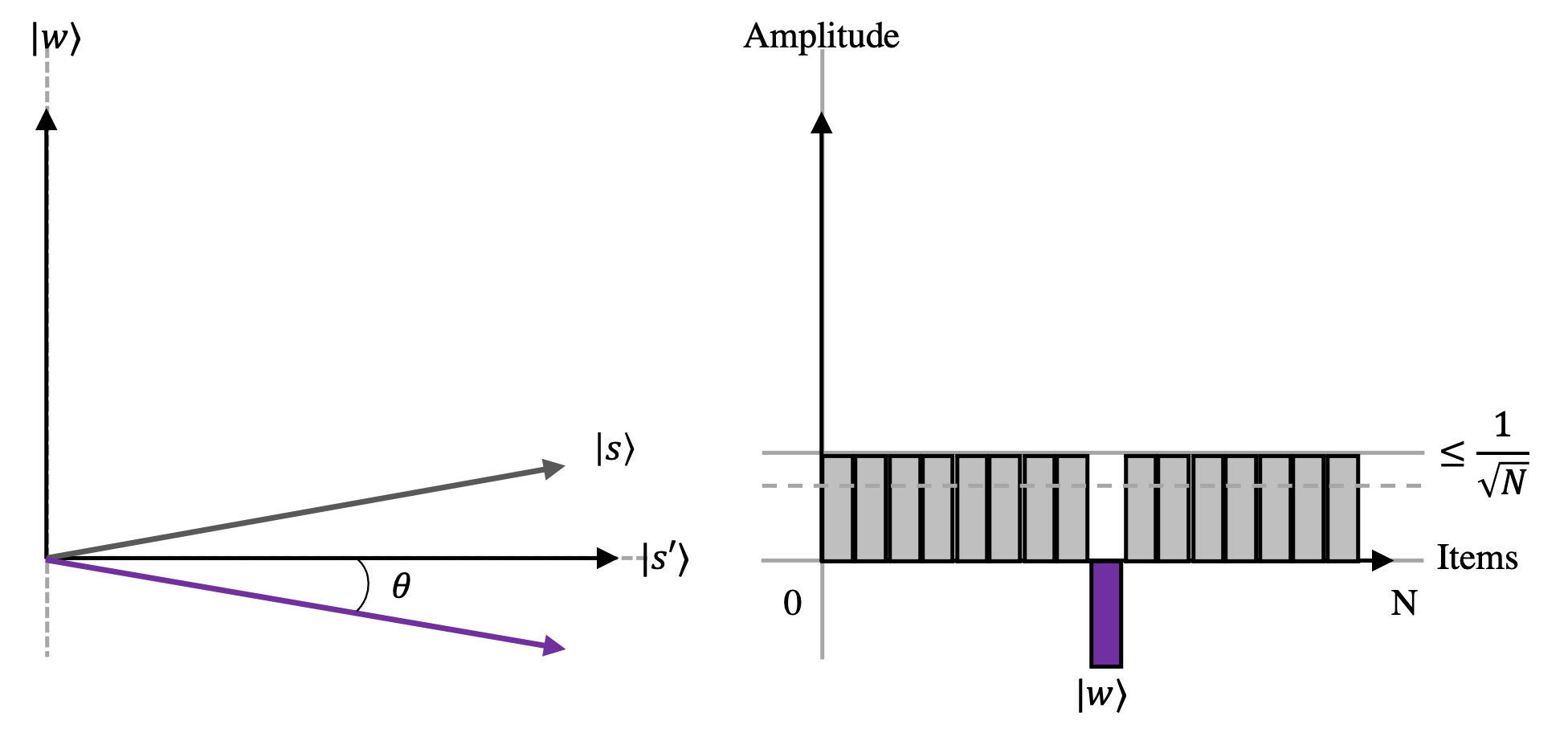
Step 3: Inversion about the mean by diffuser. Next, the diffuser circuit maps the winning state, corresponding to the marked item, to $U_{s}U_{f}\lvert s\rangle$. $U_{s}=2\lvert s\rangle\langle s\rvert-1$ corresponds to an additional rotation about the state $\lvert s\rangle$. The two reflections by $U_{f}$ and $U_{s}$ geometrically corresponds to a rotation, shown in left graphic of Figure 1(c), that brings the initial state $\lvert s\rangle$ closer towards the winner $\lvert w\rangle$. Since the average amplitude has been lowered by the first reflection, $U_{f}$, this transformation boosts the negative amplitude of $\lvert w\rangle$ to roughly three times its original value, while it decreases the other amplitudes, as shown in the right graphic of Figure 1(c).

The procedure of amplitude amplification corresponds to the combination of Step 2 and Step 3, which will be repeated several times (as shown in Figure 2) to zero in on the winner, i.e, when $\lvert s\rangle$ overlaps on $\lvert w\rangle$. It turns out the number of iterations required for this is $O(\sqrt{N})$ and thus providing a quadratic speed up over a classical counterpart.

Grover’s algorithm uses Hadamard gates, $H^{\otimes n}{\lvert 0\rangle}^{n}$ to create the uniform superposition of all the states at the beginning of the Grover operator. If some information on the good states is available, it might be useful to not start in a uniform superposition but only initialize specific states. Also, the diffusion operator does not reflect about the equal superposition state, but another state specified via an operator $\mathcal{A}$, where $\mathcal{Q}=\mathcal{A}\mathcal{S}_{0}\mathcal{A}^{\dagger}\mathcal{S}_{f}$. This generalized version of Grover’s operator ($\mathcal{Q}$) is known as Quantum Amplitude Amplification [4].

In quantum information theory, a quantum channel is a communication channel which can transmit quantum information, as well as classical information. A quantum depolarizing channel is a model for quantum noise in quantum systems. The depolarizing channel can be viewed as a completely positive trace-preserving map, $E_{\lambda}(\rho)$, which maps a mixed state $\rho$ onto a linear combination of itself and the maximally mixed state and can be defined as

When $\lambda=0$, $E_{\lambda}(\rho)=\rho$, which is the identity channel and when $\lambda=1$, $E_{\lambda}(\rho)=\frac{I}{2^{n}}$, which is a completely depolarizing channel returning maximally mixed state.

Depolarizing channel is symmetrical across all three $x$, $y$, and $z$-axes. Hence, $E_{\lambda}(\rho)$ can be interpreted as a uniform contraction of the Bloch sphere, parameterized by $\lambda$. For example, $\lambda=0$ represents the complete contraction of the Bloch-sphere down to the single-point $\frac{I}{2}$ given by the origin.

The additivity of Holevo information for all channels was a famous open conjecture in quantum information theory, but it is now known that this conjecture doesn’t hold in general. This was proved by showing that the additivity of minimum output entropy for all channels doesn’t hold [10], which is an equivalent conjecture. Nonetheless, the additivity of the Holevo information is shown to hold for the quantum depolarizing channel. Christopher King [12] showed that the maximum output p-norm of the depolarizing channel is multiplicative, which implied the additivity of the minimum output entropy, which is equivalent to the additivity of the Holevo information.

In order for the back-end transpiler to make an informed decision on whether to proceed with an iteration in the face of noise, first, it must know the amount of amplification achieved per iteration, and second, where the iteration boundaries lie in code. To this end, we propose four novel intrinsics for the OpenQASM (Open Quantum Assembly Language): $amplification\_begin(\theta)$, $amplification\_end()$, $iteration\_begin()$, and $iteration\_end()$. These intrinsics are only meant for the consumption of the transpiler and do not translate to quantum gates themselves. At below is how we would use these intrinsics in actual amplitude amplification code:

The $\theta$ is the rotational angle used in each amplification step. Iteration number $t_{opt}$ is the iteration when $\lvert w\rangle$, the winning state, is reached in the absence of noise. The $iteration\_begin()$ and $iteration\_end()$ and delineate iteration boundaries. Our amplify_optimal generates the above code after computing $\theta$ and $t_{opt}$ as shown in Method 1.

As described in Section 2.1, the amplitude amplification process starts with an initial superposition state $\lvert s\rangle=\sin(\theta)\lvert w\rangle+\cos(\theta)\lvert s^{\prime}\rangle$, where $\theta=\arcsin(\langle s\lvert w\rangle)$. For a single solution or one marked item in $N=2^{n}$ dimensional solution space, $\theta=\arcsin(\langle s\lvert w\rangle)=\arcsin(\frac{1}{\sqrt{N}})$. It can be further generalized to show that for a problem with $M$ solutions, the initial amplitude can be expressed as $\theta=\arcsin{(\sqrt{\frac{M}{N}})}$.

As described in Section 2.1, amplitude amplification is implemented as an oracle circuit followed by a diffuser circuit, which can be expressed as the transformation $U_{s}U_{f}$. To achieve a higher probability, this process is repeated several times as shown in Figure 2. The resulting state of the marked item after $t$ iterations can be expressed as $\psi_{t}=(U_{s}U_{f})^{t}\lvert s\rangle=\sin(\theta_{t})\lvert w\rangle+\cos(\theta_{t})\lvert s^{\prime}\rangle$, where $\theta_{t}=(2t+1)\theta$. The process of iterating over oracle and diffuser circuit stops when $\psi_{t}$ overlaps with the winning state, $\lvert w\rangle$. Geometrically, this means $\theta_{t}=(2t+1)\theta=\frac{\pi}{2}$. By using trigonometric identity, $\frac{\pi}{2}=\arcsin{(\theta)}+\arccos{(\theta)}$, the optimal number of iterations to attain highest outcome probability can be expressed as $t_{opt}=\frac{\arccos{(\sqrt{\frac{M}{N}})}}{2*\arcsin{(\sqrt{\frac{M}{N}})}}$. This mathematical formula is captured in Method 1.

Given amplification information through the intrinsics, now the transpiler calculates a prediction for the degradation in the winning outcome due to noise. In order to do that, we need to return to Equation 1 for the depolarizing noise channel. The mixed state $\rho$ in the equation is expressed as a density matrix, which is an ensemble of multiple pure states, each with an associated probability of occurrence. Since the probabilities of occurrence for the basis states always add up to 1, the trace of the density matrix, $Tr[\rho]=1$. Hence, the equation can be rewritten as:

To wrap our heads around this equation, let us discuss an example where $n=1$ and a depolarizing noise channel is applied to a single qubit sx gate, where the circuit looks like Figure 4(a). Since $I=\lvert 0\rangle\langle 0\lvert+\lvert 1\rangle\langle 1\lvert$, $\rho$ can be expressed as an ensemble of three states: the original state (Figure 4(a)), the basis state $\lvert 0\rangle$ (Figure 4(b)), and the basis state $\lvert 1\rangle$ (Figure 4(c)), with probabilities $1-\lambda$, $\lambda/2$, and $\lambda/2$ respectively.

When $\lambda=0$, that is when there is no error, the sx gate is unaffected and always functions like the original circuit  4(a). When $\lambda=1$, $\rho$ becomes a maximally mixed state $\frac{1}{2}(\lvert 0\rangle\langle 0\lvert+\lvert 1\rangle\langle 1\lvert)$, where there is equal probability of the circuit functioning like  4(b) or  4(c).

When $n=2$ and a depolarizing noise channel is applied to a two qubit gate such as cx gate, the ensemble of states in $\rho$ looks like Figure 5. In this case, $I=\lvert 00\rangle\langle 00\lvert+\lvert 01\rangle\langle 01\lvert+\lvert 10\rangle\langle 10\lvert+\lvert 11\rangle\langle 11\lvert$. So, we will obtain an ensemble of five states: the original state (Figure 5(a)), the basis state $\lvert 00\rangle$ (Figure 5(b)), the basis state $\lvert 01\rangle$ (Figure 5(c)), the basis state $\lvert 10\rangle$ (Figure 5(d)), and the basis state $\lvert 11\rangle$ (Figure 5(e)).

We verified our understanding of the depolarizing error channel by experimenting with many microcircuits on IBM Qiskit. We verified that the outcome of a circuit when applied depolarizing noise is actually equivalent to the sum of the outcomes of the ensemble circuits weighted by probability, as described in Figure 4 and Figure 5.

Given our understanding of the depolarizing error channel now, we would like to calculate error probability $P$ from depolarizing error parameter $\lambda$. It is easy to mistakenly think that $P=\lambda$ from the construction of Equation 2. However, things are not that simple.

Let’s again start by reasoning about depolarizing error for $n=1$. $P$ denotes the probability that a random rotation is performed on the qubit due to depolarizing noise. The rotation can happen with equal probability on the X, Y, and Z axes in the Bloch sphere, giving us the equation:

Now, how is Equation 3 related to Equation 2 which is parameterized by $\lambda$ instead of $P$? We know that by Pauli twirling we can achieve the maximally mixed state $\frac{I}{2}$:

If we apply Equation 4 to Equation 3:

Comparing that to $E_{\lambda}(\rho)=(1-\lambda)\rho+{\lambda}{\frac{I}{2^{n}}}$ in Equation 2, it is easy to derive the equality:

Now Equation 3 can be generalized to an arbitrary $n$:

Also, the Pauli twirl can be generalized to $n$ qubits as well:

Applying Equation 8 to Equation 7, the following is derived:

Finally, comparing Equation 9 against Equation 2, we derive generally for $n$ the value of $P$:

A quantum machine back-end advertises the noise parameters ($\lambda$s) for each physical gate in the machine in a long table. From these $\lambda$s, we can apply Equation 10 to convert them to individual noise rates.

Our transpiler extension uses these noise rates to calculate the noise for the given iteration circuit as shown in Method 2. It returns the amount of degradation in probability suffered by the winning outcome due to noise for the given iteration. The function $calculate\_noise$ takes a circuit $C$ as an argument which is the circuit between the $iteration\_begin$ and $iteration\_end$ intrinsics. The circuit would contain the oracle and diffuser transformations for that iteration.

The function loops over all gates $g$ in the circuit and retrieves the corresponding $\lambda$ from the aforementioned long table and uses Equation 10 to convert it to a noise rate $p$, substituting $n$ for 1 or 2 depending on whether $g$ is a one-qubit-gate or a two-qubit-gate. Next, we use Bayes’ theorem to add $p$ to the total $noise\_rate$ for the given incremental circuit $C$.

Now, we are finally able to predict the inflection point where further iterations do not increase accuracy. In other words, we are trying to find the optimal number of iterations where the probability of the marked item is the highest. Function $optimize\_circuit$ in Method 3 takes as arguments: circuit $C$, the entire amplification circuit between the $amplification\_begin(\theta)$ and $amplification\_end()$ intrinsics, and $\theta$ which is the rotational angle passed to $amplification\_begin(\theta)$. $optimize\_circuit$ loops over all iterations of circuit $C$ until it finds the inflection point. We use variable $t$ to keep track of our current iteration.

At each iteration, first we calculate $amplification$, which is the probability of the winning outcome after $t$ iterations, in a noiseless environment. Recall from Section 2.1 that the probability of the state corresponding to the marked item being collapsed on the winning state, $\lvert w\rangle$, during the measurement is the projection of the state vector on the $\lvert w\rangle$ axis at any given time. Thus, $amplification=\sin^{2}{\theta_{t}}=\sin^{2}{(2t+1)\theta}=\sin^{2}{((2t+1)*\arcsin{(\sqrt{\frac{M}{2^{n}}})})}$.

Next the circuit for iteration $t$ is extracted from $C$ and assigned to $C_{t}$. We use $C_{t}$ to calculate $noise_{t}$ incurred from that iteration using Method 2, which we accumulate into $noise$, again using Bayes’ theorem.

When $noise$ trumps $amplification$, we have found our inflection point. At that point, we remove all remaining iterations from circuit $C$ and then return the optimized circuit.

Note that there is a potential for inaccuracy in Method 3 however. We conservatively assumed that none of the noisy results included in $noise$ would end up in the winning state. Some noisy results may in fact end up in the winning state. But we will show in our results that this inaccuracy is minimal.

The methods presented in Section 4 are implemented as part of AmplitudeAmplifier and Grover class of IBM Qiskit v0.20.2 library [1]. To evaluate the efficacy of the method predicting the optimal iteration, we used Grover’s amplitude amplification algorithm to solve a Boolean satisfiability (SAT) problem. We will publish the concrete implementation of the methods described in Section 4 along with the SAT solver quantum workloads upon acceptance. The test setup allows the flexibility to vary the number of qubits, $n$ and the number of solutions, $M$ to compose the SAT solver. Users can also pass as input argument the marked item(s) for the SAT solver. We specifically experimented with 1-SAT and 3-SAT problem by setting $M$ to 1 and 3 respectively. We will focus on 1-SAT mostly and report three variations of 1-SAT with different numbers of qubits, for $n=5$, $n=7$, and $n=9$. This is done to test our framework on different circuit sizes as shown in Table 1. We will show results for 3-SAT along with an Un-Ordered Search (UOS) benchmark later in this section.

IBM Qiskit provides a PhaseOracle class simplifying the creation of an oracle circuit from a Boolean expression and an AmplificationProblem class to compose a SAT-solver problem from the created oracle. The Grover class, which extends the general AmplitudeAmplifier, can be instantiated and then its amplify method used to amplify the amplitude of the item marked by the oracle. The Grover object can be instantiated to specify the number of iterations that the Grover operator should be applied. Users can also specify a QuantumInstance, while instantiating the Grover object, which is used to execute the transpiled circuit for a specified iteration number. We report results of execution on a noise-free aer_simulator backend and a qasm_simulator backend to model a noisy quantum resource. Both of these backends are built while limiting the basis gates to an identical set composed of sx, rz, and cx gates, such that both will produce identical transpiled circuits given the same quantum program.

To model a noisy quantum resource, we used a quantum depolarizing channel. When creating the noise model for the qasm_simulator backend, the noise parameters are set for sx, rz, and cx basis gates as the transpiled circuit is composed of these gates alone. To reduce variability in the results, we specified a sufficiently large value for the number of shots while creating the backend. We repeatedly ran each experiment several times to verify that the variability is indeed negligible and we have a statistically meaningful result.

We performed two sensitivity studies to understand the effect of noise on the probability of top outcome: (i) varying the type of noisy quantum gates, and (ii) varying the dimensionality of the problem or number of qubits. The results are shown in Figure 6 and 7 respectively. In each sub-figure, probability of the winning outcome is plotted against the number of iterations of amplitude amplification for three types of scenarios - (i) a completely noise-free simulation (shown by black solid line), (ii) the probability observed in noisy simulation by executing the transpiled circuit (shown by colored solid line), and (iii) the estimate probability of the winning outcome being noise free (shown by colored dashed line). Each subplot contains multiple lines corresponding to the simulated and estimated probabilities for varied noise parameter to understand - (i) the correlation between the number of qubits and the value of noise parameters, (ii) the correlation between the number of iterations and the value of noise parameters, and (iii) the correlation between the value of noise parameters and the outcome probability and in turn the optimal number of iteration where the peak probability is attained.

Inflection point. It is rather apparent in both Figure 6 and 7 that there exists an inflection point iterating beyond which degrades the performance irrespective of - (i) the number of qubits to solve the problem, (ii) what type of quantum gates, noise is applied to, and (iii) the value of noise parameters. This reinforces our primary hypothesis motivating this work. However, the inflection point or the optimal number of iteration shifts further away from the theoretical optimal number of iterations in a noise-free environment with more number of qubits and higher value for noise paramater.

Strong correlation between simulation and estimation. We can also see that dashed, coloured lines closely resemble the solid, coloured lines. Note that the former corresponds to the collection of winning probabilities of being noise-free estimated by our proposed methods and the latter corresponds to the probability of correct outcome being observed from simulating a transpiled circuit. This strong correlation solidifies the usability of the estimated metric to predict the optimal number of iterations. However, there is always a gap between the solid and dashed coloured lines as they are measuring two different metrics. Note that in actual simulation the noise can result in some shots to be aligned with the winning output and this dynamic behavior is next to impossible to capture without an actual execution of the transpiled circuit. Hence, the probability of winning outcome obtained from a simulation is always slightly higher than the estimated probability of top-outcome being “noise-free".

Accuracy of prediction. Table 3 summarizes the experimental results by listing the optimal number of iterations observed in a noisy simulation and predicted by Method 3 along with the probability of the winning outcome at both iterations reported by simulation for varied number of qubits and depolarizing noise parameters. We can see that the predicted value of optimal number of iterations is most of the times either same as the observed value or off by one. However, in some case with higher error rate, the predicted optimal number of iteration can be lower by up to three iterations from the optimal number of iterations reported by simulation, e.g., for problem composed of $9$ qubits and the sx and cz noise parameters respectively being $0.01$ and $0.0001$, the optimal number of iterations reported by simulation and predicted by Method 3 are $7$ and $4$ respectively where the theoretical optimal number of iterations is $17$ in a noise-free environment. However, an interesting observation is that the outcome probability reported by simulation for iterations $7$ and $4$ are extremely close ($0.08\%$ and $0.06\%$ respectively). This observation is uniform throughout several data-points. It means that even when the user choose to simulated for the predicted number of iterations for amplitude amplification, there is not a significant loss from the peak attainable probability of the winning outcome.

Correlation between the noise parameters, the number of qubits, and the number of gates. It is interesting to note that the depolarizing noise parameter single-qubit gate is varied from $0.002$ to $0.01$ in the increment of $0.002$ for experiments irrespective of the dimensionality of the problem. This is however not true for two-qubit quantum gates. The noise parameter for cx gates ranges from $0.002$ to $0.01$ for $5$ qubit circuits, whereas they are two-order of magnitude smaller ranging from $2\times 10^{-5}$ to $1\times 10^{-4}$ with increment of $2\times 10^{-5}$ for $9$-qubit circuits. This is because of two reasons. Firstly, as reported in Table 1, the number of sx gates is way smaller than the number of cx gates in a transpiled circuit and the difference grows larger with higher number of qubits, e.g., for a circuit with $9$ qubit, the number of sx gates is two-order of magnitude smaller than the number of cx gates. As a result, loss of accuracy due to noise on sx is relatively smaller than that from cx gates. Second, the number of cx gates grows by an order of magnitude from circuit with $5$ ($320$) to $7$ ($3008$) to $9$ ($25976$) qubits. So, to keep up with the growth in number of two-qubit gates with the increase in dimensionality of the problem, the noise parameter should also be scaled down by order of magnitude to yield any meaningful result and demonstrate the convex progression with an inflection point. If the value of noise-parameter is too high (e.g. noise parameters are $0.01$ and $0.0001$ for sx and cx gates in 9-qubit circuit) for the total number of quantum gates in the circuit, it results in an almost flat curve parallel to horizontal axis. This corresponds to all qubits being in a maximally mixed state where the result is uniformly random irrespective of iterating over amplitude amplification.

Evaluation on real quantum machines. We tried running our amplitude amplification programs on existing quantum machines on the IBM Quantum cloud. We found that, even with our programs using just 5 qubits, all machines had error rates that were too high to provide any meaningful results. Even after just one amplification iteration, the computation was overwhelmed by noise. The noise was exacerbated by limited machine topologies where not all pairs of qubits allow entanglement, requiring many extra swap operations to be inserted to move qubits adjacent to each other. So we decided to simulate a machine similar to ibm_oslo with identical noise model including thermal relaxation as well as depolarizing noise, except with the modification that qubits are fully connected and allow arbitrary entanglement. The results of this experiment is in Table 4. First, note that the “Predicted optimal # of iterations” occurs earlier compared to the “Theoretical optimal # of iterations”, in line with previous results. Importantly, note that the prediction is not only accurate for the “simulated environment", but also for ibm_oslo with the full noise model, the only exception being UOS (Un-Ordered Search) with a difference of 1 iteration. And even for UOS, the difference between the success probability when using our prediction (0.252) and on the actual observed optimal point (0.257) is negligible. This shows the efficacy of predicting the optimal number of iterations by our analytical model even when noise channels other than depolarizing quantum noise is present. We plan to eventually add thermal relaxation to our prediction model in future work, but we feel these are promising results.

Evaluation on other benchmarks. In Figure 8, we show the results of applying our optimization to 3-SAT and UOS (Un-Ordered Search) along with 1-SAT, using a program size of 8 qubits on a machine with single qubit and two-qubit noise rates as $0.004$ and $0.00004$ respectively. Note that, just like previous results, the observed simulation curve closely tracks our estimated prediction curve. The theoretical optimal iterations of 1-SAT, 3-SAT and UOS are 12, 7, and 12 respectively. The predicted optimal iterations (the peak of the dotted lines) are 10, 6, and 10 respectively which match exactly with the observed optimal iterations (the peak of the solid lines). This shows that our optimization is applicable to a variety of quantum algorithms that inherently repeats part of circuit with more iterations.

References

- [1] M. S. ANIS, Abby-Mitchell, H. Abraham, AduOffei, R. Agarwal, G. Agliardi, M. Aharoni, V. Ajith, I. Y. Akhalwaya, G. Aleksandrowicz, T. Alexander, M. Amy, S. Anagolum, Anthony-Gandon, E. Arbel, A. Asfaw, A. Athalye, A. Avkhadiev, C. Azaustre, P. BHOLE, A. Banerjee, S. Banerjee, W. Bang, A. Bansal, P. Barkoutsos, A. Barnawal, G. Barron, G. S. Barron, L. Bello, Y. Ben-Haim, M. C. Bennett, D. Bevenius, D. Bhatnagar, P. Bhatnagar, A. Bhobe, P. Bianchini, L. S. Bishop, C. Blank, S. Bolos, S. Bopardikar, S. Bosch, S. Brandhofer, Brandon, S. Bravyi, N. Bronn, Bryce-Fuller, D. Bucher, A. Burov, F. Cabrera, P. Calpin, L. Capelluto, J. Carballo, G. Carrascal, A. Carriker, I. Carvalho, A. Chen, C.-F. Chen, E. Chen, J. C. Chen, R. Chen, F. Chevallier, K. Chinda, R. Cholarajan, J. M. Chow, S. Churchill, CisterMoke, C. Claus, C. Clauss, C. Clothier, R. Cocking, R. Cocuzzo, J. Connor, F. Correa, Z. Crockett, A. J. Cross, A. W. Cross, S. Cross, J. Cruz-Benito, C. Culver, A. D. Córcoles-Gonzales, N. D, S. Dague, T. E. Dandachi, A. N. Dangwal, J. Daniel, M. Daniels, M. Dartiailh, A. R. Davila, F. Debouni, A. Dekusar, A. Deshmukh, M. Deshpande, D. Ding, J. Doi, E. M. Dow, P. Downing, E. Drechsler, E. Dumitrescu, K. Dumon, I. Duran, K. EL-Safty, E. Eastman, G. Eberle, A. Ebrahimi, P. Eendebak, D. Egger, ElePT, Emilio, A. Espiricueta, M. Everitt, D. Facoetti, Farida, P. M. Fernández, S. Ferracin, D. Ferrari, A. H. Ferrera, R. Fouilland, A. Frisch, A. Fuhrer, B. Fuller, M. GEORGE, J. Gacon, B. G. Gago, C. Gambella, J. M. Gambetta, A. Gammanpila, L. Garcia, T. Garg, S. Garion, J. R. Garrison, J. Garrison, T. Gates, H. Georgiev, L. Gil, A. Gilliam, A. Giridharan, Glen, J. Gomez-Mosquera, Gonzalo, S. de la Puente González, J. Gorzinski, I. Gould, D. Greenberg, D. Grinko, W. Guan, D. Guijo, Guillermo-Mijares-Vilarino, J. A. Gunnels, H. Gupta, N. Gupta, J. M. Günther, M. Haglund, I. Haide, I. Hamamura, O. C. Hamido, F. Harkins, K. Hartman, A. Hasan, V. Havlicek, J. Hellmers, Ł. Herok, S. Hillmich, C. Hong, H. Horii, C. Howington, S. Hu, W. Hu, C.-H. Huang, J. Huang, R. Huisman, H. Imai, T. Imamichi, K. Ishizaki, Ishwor, R. Iten, T. Itoko, A. Ivrii, A. Javadi, A. Javadi-Abhari, W. Javed, Q. Jianhua, M. Jivrajani, K. Johns, S. Johnstun, Jonathan-Shoemaker, JosDenmark, JoshDumo, J. Judge, T. Kachmann, A. Kale, N. Kanazawa, J. Kane, Kang-Bae, A. Kapila, A. Karazeev, P. Kassebaum, T. Kehrer, J. Kelso, S. Kelso, H. van Kemenade, V. Khanderao, S. King, Y. Kobayashi, Kovi11Day, A. Kovyrshin, R. Krishnakumar, P. Krishnamurthy, V. Krishnan, K. Krsulich, P. Kumkar, G. Kus, R. LaRose, E. Lacal, R. Lambert, H. Landa, J. Lapeyre, J. Latone, S. Lawrence, C. Lee, G. Li, T. J. Liang, J. Lishman, D. Liu, P. Liu, Lolcroc, A. K. M, L. Madden, Y. Maeng, S. Maheshkar, K. Majmudar, A. Malyshev, M. E. Mandouh, J. Manela, Manjula, J. Marecek, M. Marques, K. Marwaha, D. Maslov, P. Maszota, D. Mathews, A. Matsuo, F. Mazhandu, D. McClure, M. McElaney, C. McGarry, D. McKay, D. McPherson, S. Meesala, D. Meirom, C. Mendell, T. Metcalfe, M. Mevissen, A. Meyer, A. Mezzacapo, R. Midha, D. Miller, H. Miller, Z. Minev, A. Mitchell, N. Moll, A. Montanez, G. Monteiro, M. D. Mooring, R. Morales, N. Moran, D. Morcuende, S. Mostafa, M. Motta, R. Moyard, P. Murali, D. Murata, J. Müggenburg, T. NEMOZ, D. Nadlinger, K. Nakanishi, G. Nannicini, P. Nation, E. Navarro, Y. Naveh, S. W. Neagle, P. Neuweiler, A. Ngoueya, T. Nguyen, J. Nicander, Nick-Singstock, P. Niroula, H. Norlen, NuoWenLei, L. J. O’Riordan, O. Ogunbayo, P. Ollitrault, T. Onodera, R. Otaolea, S. Oud, D. Padilha, H. Paik, S. Pal, Y. Pang, A. Panigrahi, V. R. Pascuzzi, S. Perriello, E. Peterson, A. Phan, K. Pilch, F. Piro, M. Pistoia, C. Piveteau, J. Plewa, P. Pocreau, A. Pozas-Kerstjens, R. Pracht, M. Prokop, V. Prutyanov, S. Puri, D. Puzzuoli, Pythonix, J. Pérez, Quant02, Quintiii, R. I. Rahman, A. Raja, R. Rajeev, I. Rajput, N. Ramagiri, A. Rao, R. Raymond, O. Reardon-Smith, R. M.-C. Redondo, M. Reuter, J. Rice, M. Riedemann, Rietesh, D. Risinger, P. Rivero, M. L. Rocca, D. M. Rodríguez, RohithKarur, B. Rosand, M. Rossmannek, M. Ryu, T. SAPV, N. R. C. Sa, A. Saha, A. Ash-Saki, S. Sanand, M. Sandberg, H. Sandesara, R. Sapra, H. Sargsyan, A. Sarkar, N. Sathaye, N. Savola, B. Schmitt, C. Schnabel, Z. Schoenfeld, T. L. Scholten, E. Schoute, M. Schulterbrandt, J. Schwarm, J. Seaward, Sergi, I. F. Sertage, K. Setia, F. Shah, N. Shammah, W. Shanks, R. Sharma, P. Shaw, Y. Shi, J. Shoemaker, A. Silva, A. Simonetto, D. Singh, D. Singh, P. Singh, P. Singkanipa, Y. Siraichi, Siri, J. Sistos, I. Sitdikov, S. Sivarajah, Slavikmew, M. B. Sletfjerding, J. A. Smolin, M. Soeken, I. O. Sokolov, I. Sokolov, V. P. Soloviev, SooluThomas, Starfish, D. Steenken, M. Stypulkoski, A. Suau, S. Sun, K. J. Sung, M. Suwama, O. Słowik, H. Takahashi, T. Takawale, I. Tavernelli, C. Taylor, P. Taylour, S. Thomas, K. Tian, M. Tillet, M. Tod, M. Tomasik, C. Tornow, E. de la Torre, J. L. S. Toural, K. Trabing, M. Treinish, D. Trenev, TrishaPe, F. Truger, G. Tsilimigkounakis, D. Tulsi, D. Tuna, W. Turner, Y. Vaknin, C. R. Valcarce, F. Varchon, A. Vartak, A. C. Vazquez, P. Vijaywargiya, V. Villar, B. Vishnu, D. Vogt-Lee, C. Vuillot, J. Weaver, J. Weidenfeller, R. Wieczorek, J. A. Wildstrom, J. Wilson, E. Winston, WinterSoldier, J. J. Woehr, S. Woerner, R. Woo, C. J. Wood, R. Wood, S. Wood, J. Wootton, M. Wright, L. Xing, J. YU, Yaiza, B. Yang, U. Yang, J. Yao, D. Yeralin, R. Yonekura, D. Yonge-Mallo, R. Yoshida, R. Young, J. Yu, L. Yu, Yuma-Nakamura, C. Zachow, L. Zdanski, H. Zhang, I. Zidaru, B. Zimmermann, C. Zoufal, aeddins ibm, alexzhang13, b63, bartek bartlomiej, bcamorrison, brandhsn, chetmurthy, deeplokhande, dekel.meirom, dime10, dlasecki, ehchen, ewinston, fanizzamarco, fs1132429, gadial, galeinston, georgezhou20, georgios ts, gruu, hhorii, hhyap, hykavitha, itoko, jeppevinkel, jessica angel7, jezerjojo14, jliu45, johannesgreiner, jscott2, kUmezawa, klinvill, krutik2966, ma5x, michelle4654, msuwama, nico lgrs, nrhawkins, ntgiwsvp, ordmoj, sagar pahwa, pritamsinha2304, rithikaadiga, ryancocuzzo, saktar unr, saswati qiskit, septembrr, sethmerkel, sg495, shaashwat, smturro2, sternparky, strickroman, tigerjack, tsura crisaldo, upsideon, vadebayo49, welien, willhbang, wmurphy collabstar, yang.luh, and M. Čepulkovskis, “Qiskit: An open-source framework for quantum computing,” 2021.
- [2] D. Bera, “Amplitude amplification for operator identification and randomized classes,” in International Computing and Combinatorics Conference. Springer, 2018, pp. 579–591.
- [3] G. Brassard and P. Hoyer, “An exact quantum polynomial-time algorithm for simon’s problem,” in Proceedings of the Fifth Israeli Symposium on Theory of Computing and Systems. IEEE, 1997, pp. 12–23.
- [4] G. Brassard, P. Hoyer, M. Mosca, and A. Tapp, “Quantum amplitude amplification and estimation,” Contemporary Mathematics, vol. 305, pp. 53–74, 2002.
- [5] I. Cohn, A. Fonseca de Oliveira, E. Buksman, and J. Lacalle, “Grover’s search with local and total depolarizing channel errors: Complexity analysis,” International Journal of Quantum Information, vol. 14, no. 2, p. 1650009, 2016.
- [6] D. Daoyi, C. Chunlin, and L. Hanxiong, “Reinforcement strategy using quantum amplitude amplification for robot learning,” in 2007 Chinese Control Conference. IEEE, 2007, pp. 571–575.
- [7] B. Elias and A. Younes, “Enhanced quantum signature scheme using quantum amplitude amplification operators,” PloS one, vol. 16, no. 10, p. e0258091, 2021.
- [8] R. Franco, “Quantum amplitude amplification algorithm: an explanation of availability bias,” in International Symposium on Quantum Interaction. Springer, 2009, pp. 84–96.
- [9] L. K. Grover, “A fast quantum mechanical algorithm for database search,” in Proceedings of the twenty-eighth annual ACM symposium on Theory of computing, 1996, pp. 212–219.
- [10] M. B. Hastings, “Superadditivity of communication capacity using entangled inputs,” Nature Physics, vol. 5, no. 4, pp. 255–257, 2009.
- [11] IBM Q team, “IBM Q backend specification,” https://quantum-computing.ibm.com.
- [12] C. King, “The capacity of the quantum depolarizing channel,” IEEE Transactions on Information Theory, vol. 49, no. 1, pp. 221–229, 2003.
- [13] D. Koch, M. Cutugno, S. Karlson, S. Patel, L. Wessing, and P. M. Alsing, “Gaussian amplitude amplification for quantum pathfinding,” Entropy, vol. 24, no. 7, p. 963, 2022.
- [14] D. Kravchenko, N. Nahimovs, and A. Rivosh, “Grover’s search with faults on some marked elements,” in International Conference on SOFSEM 2016: Theory and Practice of Computer Science. ACM, 2016.
- [15] H. Kwon and J. Bae, “Quantum amplitude-amplification operators,” Physical Review A, vol. 104, no. 6, p. 062438, 2021.
- [16] D. C. McKay, C. J. Wood, S. Sheldon, J. M. Chow, and J. M. Gambetta, “Efficient z gates for quantum computing,” Physical Review A, vol. 96, no. 2, p. 022330, 2017.
- [17] B. Pablo-Norman and M. Ruiz-Altaba, “Noise in grover’s quantum search algorithm,” Physical Review A, vol. 61, no. 1, 1999.
- [18] K. Rajagopal, Q. Zhang, S. Balakrishnan, P. Fakhari, and J. Busemeyer, “Quantum amplitude amplification for reinforcement learning,” Handbook of Reinforcement Learning and Control, pp. 819–833, 2021.
- [19] A. Rastegin, “On degradation of grover’s search under collective phase flips in queries to the oracle,” Frontiers of Physics, vol. 13, 2017.
- [20] D. Reitzner and M. Hillery, “Grover search under localized dephasing,” Physical Review A, vol. 99, p. 012339, 2019.
- [21] Y. Wang and P. S. Krstic, “Prospect of using grover’s search in the noisy-intermediate-scale quantum-computer era,” Physical Review A, vol. 102, p. 042609, 2020.
- [22] K. Zhang and V. E. Korepin, “Depth optimization of quantum search algorithms beyond grover’s algorithm,” Phys. Rev. A, vol. 101, p. 032346, 2020.