A New Quantization Principle
from a Minimally
non Time-Ordered Product
Damiano Anselmi
Dipartimento di Fisica “E.Fermi”, Università di Pisa, Largo B.Pontecorvo 3, 56127 Pisa, Italy
INFN, Sezione di Pisa, Largo B. Pontecorvo 3, 56127 Pisa, Italy
damiano.anselmi@unipi.it
Abstract
We formulate a new quantization principle for perturbative quantum field theory, based on a minimally non time-ordered product, and show that it gives the theories of physical particles and purely virtual particles. Given a classical Lagrangian, the quantization proceeds as usual, guided by the time-ordered product, up to the common scattering matrix , which satisfies a unitarity or a pseudounitarity equation. The physical scattering matrix is built from , by gluing diagrams together into new diagrams, through non time-ordered propagators. We classify the most general way to gain unitarity by means of such operations, and point out that a special solution “minimizes” the time-ordering violation. We show that the scattering matrix given by this solution coincides with the one obtained by turning the would-be ghosts (and possibly some would-be physical particles) into purely virtual particles (fakeons). We study tricks to descend and ascend in a unique way among diagrams, and illustrate them in several examples: the ascending chain from the bubble to the hexagon, at one loop; the box with diagonal, at two loops; other diagrams, with more loops.
1 Introduction
Unitarity is a fundamental principle of quantum field theory. It states that the scattering matrix satisfies the unitarity equation . Equivalently, the matrix defined by satisfies the optical theorem
| (1.1) |
The virtue of this formula is that it can be converted into Cutkosky-Veltman identities [1, 2, 3, 4], which are diagrammatic relations, satisfied by each diagram separately. The diagrams of are built by means of the usual vertices and propagators. The diagrams of are built by means of the conjugate vertices and the conjugate propagators. The diagrams of have two sides, one for and one for , separated by a “cut”. The product between and is rendered diagrammatically by means of “cut propagators”, which are on shell and encode the physical contents of the theory.
Thus, while the matrix is given by the usual Feynman diagrams, the identity (1.1) involves the larger class of Cutkosky-Veltman diagrams, which are also called “cut diagrams”. It was shown in ref. [5] that the identities obeyed by the “skeletons” of the diagrams (where we ignore the integrals on the space components of the loop momenta) split into independent spectral optical identities, one for every (multi)threshold. The virtue of these relations is that they are algebraic and relatively straightforward to manipulate. Moreover, they provide the threshold decomposition of a diagram, which can be used to quantize the would-be ghosts, and possibly some would-be physical particles, as purely virtual particles, thereby projecting the matrix onto a reduced matrix , which may be physically acceptable even if is not.
Purely virtual particles, also called fake particles, or fakeons, are defined by this new diagrammatics [5]. The projection allows us to remove degrees of freedom from the physical spectrum at all energies, and satisfy the optical theorem in a manifest way. The main application of the idea is the formulation of a consistent theory of quantum gravity [6], which is observationally testable due to its predictions in inflationary cosmology [7]. At the phenomenological level, fakeons evade common constraints that limit the employment of normal particles (see [8] and references therein).
In this paper, we study the scattering matrix of quantum field theory under a new light. We inquire what transformations we can make on the usual matrix, which is defined by the time-ordered product, to turn it into a different scattering matrix , possibly better suited to describe the physics we observe in experiments. We end up by uncovering purely virtual particles again, in an independent way. The results confirm and upgrade the ones of [5] and provide an alternative understanding of the concept of purely virtuality.
Unitarity is not an automatic consequence of the usual quantization principle, and should not be taken for granted. For example, if we start from a theory that contains fields with negative kinetic terms, and quantize it as usual, we obtain a matrix that is not physically acceptable, because it does not satisfy the unitarity equation (1.1). Even in that case, though, satisfies a mathematically useful identity, which reads [3, 4]
| (1.2) |
and is called pseudounitarity equation, where is a diagonal matrix with eigenvalues equal to 1, 1 and possibly 0 (if auxiliary fields are present). Higher-derivative theories are typical examples of theories satisfying (1.2) with .
Normally, the quantization ends with the matrix, which means that if is physically unacceptable the theory is discarded. What if the quantization did not end there? What if the derivation of were just the first step of a longer, more elaborate quantization procedure? To make this happen, we need a new quantization principle, equivalent to the old one whenever the old one was successful, but possibly differing from it in every other case. In particular, it should contemplate a second step, defined by new diagrammatic rules, and a map from the “interim” matrix satisfying (1.2), to the “finalized”, hopefully physical, matrix , satisfying (1.1).
The first task is to classify all the possibilities we have to build a unitary scattering matrix from another unitary scattering matrix, or from a pseudounitary one, . Since the time-ordered product leads to the usual matrix, and leaves no room for alternatives, the second part of the new quantization principle must be based on non time-ordered products.
The set of solutions to the problem just stated is large, but a very special one can be singled out among the others. It is the one that minimizes, so to speak, the violation of the time ordering. A bonus is that it provides an alternative way to uncover the physics of purely virtual particles.
The new quantization principle
We briefly describe the new diagrammatics, and state the quantization principle they lead to. If denotes the fields, the diagrams of the physical matrix are built by means of the usual vertices, the usual (time-ordered) free-field propagators
| (1.3) |
and the non time-ordered free-field propagators
| (1.4) |
The rules to build the diagrams with these ingredients are encoded into a compact formula, which is eq. (2.16) of section 2, and an iterative procedure to eliminate a certain arbitrariness contained in that same formula.
Curiously enough, the non time-ordered propagators (1.4) coincide with the cut propagators mentioned earlier. However, the cut propagators are not used to build the diagrams, which define the ordinary transition amplitudes. They appear in the Cutkosky-Veltman diagrams, when we study the (pseudo)unitarity equations (1.1) and (1.2) obeyed by . Specifically, they connect and through the products appearing on the right-hand sides of those equations. The first, crucial novelty of the new diagrammatics is that the non time-ordered propagators (1.4) are ingredients of the diagrams that give the physical transition amplitudes, collected in . This way, the physical scattering matrix is no longer dictated by the time-ordered product. The inclusion of non time-ordered propagators multiplies the number of diagrams we have to consider by a large factor. However, the new diagrams are not more difficult than the usual ones, and their large number can be easily dealt with by means of computer programs, like the popular ones used nowadays in phenomenology [9].
Briefly, the usual diagrams contributing to are glued together in certain, prescribed ways, by means of the non time-ordered propagators, to build the new diagrams, those of . A certain formula mapping the standard matrix to the physical matrix , and a certain procedure, guide the assembly of the new diagrams.
The new quantization principle is thus made of two parts. The first part amounts to build the matrix as usual. The second part amounts to work out the physical matrix as explained. The map is sometimes called “projection”, other times “reduction”, interchangeably.
We show that the most general reduced matrix built from , which obeys the unitarity equation, depends on an arbitrary anti-Hermitian matrix . A special is singled out by requiring that the projection of a product diagram is equal to the product of the projected factors, and the factorization survives basic diagrammatic operations. Due to the violation of time ordering, this factorization requirement is nontrivial. It amounts to assume that the violation is a “minimum” one, rather than the most brutal one: it is confined inside non factorizable diagrams, which we call “prime” diagrams. The reason why we call it minimum violation is that it does not seem possible to violate it less than this. With this particular choice of , the large number of diagrams collapses to an amount that is comparable to the one generated by the usual time-ordered product.
We show that the reduced matrix obtained this way coincides with the matrix of a theory of physical and purely virtual particles, as given in ref. [5]. Once we decide which particles we want to quantize as physical and which ones we want to quantize as purely virtual, follows uniquely.
We briefly mention the other results of the paper. We work out a number of tricks to descend from bigger to smaller diagrams, but also ascend in a unique way from smaller to bigger diagrams, and relate their corrections and their threshold decompositions. We illustrate these properties in various examples. At one loop, we study the ascending chain
At two loops, we focus on the first nontrivial arrangement, which is the box diagram with diagonal. Classes of diagrams with arbitrarily many loops are also discussed. Agreement with the formulas of [5] is found in every example.
A diagram may need an overall correction, but also inherit corrections from its subdiagrams. In all the cases we consider, nontrivial corrections are present when the diagram is not prime, and also when it is prime, but factorizes under the contraction of some internal legs. We find that it is always possible to ascend through the threshold decompositions in a unique way. We conjecture that these are general properties of the physical matrix .
Since the time-ordered product is not a physical principle, we should be open to the possibility that the physical laws may break it, one way or another. Purely virtual particles provide the most elegant and economic way of implementing such a breaking. In physical applications, purely virtual particles are expected to be massive, and generically heavy. For example, one spin-2 purely virtual particle of mass 1012-13GeV is enough to make sense of quantum gravity [6]. In that case, the violation of time ordering is restricted to distances , and so is the violation of microcausality associated with it (as well as the violation of microlocality, when is integrated out). Tiny violations like these are not detectable in realistic situations, even if we take into account the possibility of boosting the systems. We also recall that purely virtual particles in curved space lead to a sharp prediction for the tensor-to-scalar ratio in primordial cosmology ( [7]). The first observational results on this are expected to become available in the present decade [10].
The results of this paper provide a quantization, in perturbation theory, of any theory for which the usual Feynman diagram calculation of the matrix gives a result satisfying (1.2). In particular, no assumption about gauge invariance is used. This means that we can make sense of a very wide class of theories usually thought unacceptable. Many workers in quantum field theory believe that negative probability modes can only be removed if the theory has a gauge invariance, and that the physical states are selected through that symmetry. The construction of this paper provides counterexamples to that belief.
Ultimately, the correctness of the new ideas must be proven by experiment, for example by confirming the prediction for , or the viability of standard model extensions such as the one of [11]. If theories constructed with these methods turn out to be phenomenologically correct, then we need to expand our orthodox ideas about fundamental physics. Further insight on this aspect could come from the investigation of an important open problem, that is to say, establish whether the matrix generated by the prescription for purely virtual particles is the result of a Hamiltonian evolution, as we normally understand it, or we need to relax the basic axioms of quantum mechanics. Although this issue is beyond the scope of this paper, it ought to be explored.
The paper is organized as follows. In section 2 we work out the most general map that converts a matrix satisfying the (pseudo)unitarity equation (1.2) into a reduced matrix that satisfies the unitarity equation (1.1). In section 3 we outline the basic rules for the new diagrams. In sections 4 and 5, we discuss the reduction in the cases of tree and disconnected diagrams. In section 6 we study the simplest one-loop diagrams (bubble, triangle and box). In section 7 we study diagrams with more loops, focusing on the box with diagonal, which is the first truly new arrangement. In section 8 we discuss a number of tools to have control on pure virtuality, and relate smaller and bigger diagrams. In section 9 we explain how to use those tricks to ascend and descend through the diagrams and their threshold decompositions. In section 10 we summarize the diagrammatic rules, and compare the main options (Feynman diagrams, Cutkosky-Veltman diagrams, and the diagrams defined here), and their uses. In section 11 we show that the projection preserves the global and local symmetries of a theory, the cancellation of anomalies and the renormalizability. Section 12 contains the conclusions. In appendix A we explain how to switch from the scattering matrix to single diagrams, without loss of information, and vice versa, to derive the diagrammatic identities. In appendix B we prove some identities for product distributions, used in the paper.
2 The key issue and its solution
In this section we describe how to reduce the scattering matrix of a possibly nonunitary theory to a unitary scattering matrix. We classify the set of solutions without assuming physical inputs.
We decompose the usual matrix as
| (2.1) |
where , and collects the common transition amplitudes, defined by the time-ordered product. From now on, we refer to , or, more generally, the difference between a scattering matrix and the identity matrix, by simply calling it “amplitude”.
The unitarity of the matrix, i.e., the identity , gives the identity
| (2.2) |
for the amplitude . Various quantum field theories do not allow us to prove an equation of this form right away. When the theory has fields with negative kinetic terms, we can just prove a pseudounitarity equation
| (2.3) |
where is some Hermitian matrix. We can diagonalize and normalize so as to put it into the form
| (2.4) |
The corresponding Fock space decomposition is written as , where is the total Fock space.
A quick derivation of (2.3) from (2.2) goes on as follows. We integrate out the auxiliary fields, for simplicity, and use to denote the fields that have negative kinetic terms. If, for a moment, we change the signs of the propagators, we obtain a modified theory that satisfies (2.2). Consider a diagram of the modified theory, and the diagrammatic equation satisfied by it, generated by (2.2). If we multiply that equation by a factor , where denotes the number of the legs, we restore the factors of the original theory in front of the propagators of the internal legs due to and . However, the cut legs connecting and also get factors . This converts the unit matrix between and into the matrix , leading to formula (2.3).
Our goal is to project the amplitude and the space , so as to obtain an equation like (2.2) from (2.3), holding in a “physical” subspace of .
Let
| (2.5) |
denote the projector onto , and the corresponding decomposition, where , . It is enough to find a reduced amplitude that solves the equation
| (2.6) |
Indeed, this equation implies that the physical amplitude solves
| (2.7) |
so the physical matrix satisfies . In other words, if we manage to solve (2.6), we achieve unitarity in the subspace . Then we can legitimately claim that is the physical amplitude, and is physical space of the theory.
Summarizing, our goal is to find the most general solution of (2.6), given the physical projector .
We can generalize the problem a little bit with no effort: given Hermitian matrices and , and given a matrix that satisfies (2.3), we want to find the most general solution of the equation
| (2.8) |
This is a merely mathematical problem about matrices, and , do not need to be projectors or linear combinations of projectors. For convenience, we write
| (2.9) |
A particular solution of (2.8) is , where
| (2.10) |
This formula can be understood recursively as
Note that, despite its appearance, the solution is left-right symmetric, since we can also write
The proof that (2.10) solves follows straightforwardly from the identities
| (2.11) |
Starting from the particular solution (2.10), we can write the most general solution as
| (2.12) |
In order to fulfill (2.10), the matrix must satisfy the equation
| (2.13) |
As before, we can solve this equation recursively in powers of , starting from an arbitrary anti-Hermitian matrix that is at least of order . Indeed, if we write , with and assume that is of higher order in the expansion, we obtain the equation
which can be solved iteratively as claimed. This also proves that the matrix parametrizes the most general solution of (2.13).
It is simple to show that the explicit solution of (2.13), and its inverse, are
| (2.14) |
The proof follows by writing (2.13) in the form , where
Using the expression (2.14) of , and , we see that the matrix
is indeed anti-Hermitian.
The solution (2.12), with given in (2.10) and given in (2.14), needs some rearrangement, since it is not written in a manifestly left-right symmetric form. The symmetrization can be obtained by redefining within the realm of its own arbitrariness. Define
| (2.15) |
It is easy to prove that is anti-Hermitian. To this purpose, note that, since solves (2.8), we have the formula
Equipped with (2.15), the first expression of (2.14) can be recast into the form
which is manifestly left-right symmetric. Then, so is (2.12).
Going back to formula (2.12) and summarizing the results we have found so far, we have proved that, given a matrix that satisfies
where and are arbitrary Hermitian matrices, the most general matrix that satisfies
and coincides with up to corrections of higher orders in itself, is , where
| (2.16) |
and is an arbitrary anti-Hermitian matrix, to be considered of order two in , or higher. Formula (2.16) is the key formula of the paper.
An interesting case is when the physical space is just made of the vacuum state . Then is and is . If has the form (2.4), the solution can be used to remove the whole on-shell contents of the diagrams, and describe the situation where every particle is rendered purely virtual. To achieve this goal, must be determined so as to remove any residual on-shell contributions. As we are going to show in the next sections, this is a nontrivial task, but has a well defined answer. Unfortunately, the answer is not just . Indeed, the solution
| (2.17) |
turns out to be correct only in a certain subset of simpler diagrams. In general, a nonvanishing is to be expected. We will show that the solution , equipped with the right , provides an alternative way to make the threshold decomposition of [5].
By affinity with the notion of prime number, we say that a diagram is prime if it cannot be factorized as a nontrivial product of smaller diagrams, in momentum space. We show that, for arbitrary , can be chosen to make obey the following factorization property: the projection of a non prime diagram is the product of the projections of its prime factors, and the factorization survives basic operations of ascent and descent among diagrams. This is a nontrivial requirement, in the realm of non time-ordered products. We also show that the amplitude determined by this gives precisely the diagrams of physical and purely virtual particles, as per ref. [5]. We identify such a with the physical amplitude .
We first proceed by explicit examples, then gather the lessons we learn along the way.
3 Diagrams: the old and the new
In this section we lay out the rules to build the new diagrams, and compare them with the Feynman rules.
So far, we have been merely playing with matrices: the theorems proved in the previous section hold under assumptions that are more general than the ones we need for physical applications. To move forward towards the physics, let collect all the fields, which include the physical fields and the fields we want to project away (for one reason or another). The physical subspace contains the vacuum state and the states that are built by means of the creation operators, but no creation operators. The complementary subspace contains the states that are built by means of at least one creation operator. The idea is that a single excitation due to the fields that we want to get rid of is sufficient to drop the whole state from the physical spectrum.
From our definition (2.1), it follows that the amplitude collects the usual Feynman diagrams. In operatorial notation,
| (3.1) |
where is the interaction Hamiltonian and denotes the time-ordered product.
The diagrams are defined by the usual Feynman rules. In particular, the free-field propagators are the time-ordered ones, given by the Feynman prescription. For scalars , we have
| (3.2) |
The propagators of the fields are the same, apart from the possibility of being multiplied by minus signs. Thus, scalars may have propagators
| (3.3) |
The 0 eigenvalues of the matrix of (2.4) correspond to auxiliary fields . From now on, we assume that they are integrated away.
The right-hand side of formula (2.3) collects the usual Cutkosky-Veltman diagrams, which are graphically rendered by means cut diagrams. The cut is unique, and represents the matrix separating from . While the diagrams are time-ordered, and the diagrams are anti-time-ordered, the product is just a plain (non time-ordered) product of field operators. This means that, when we apply Wick’s theorem, the Wick contraction between a field that belongs to a conjugate vertex of , and a field that belongs to an ordinary vertex of is the non time-ordered two-point function
| (3.4) |
where the sign is or according to the sign of the eigenvalue associated with , as in (3.2) and (3.3). In momentum space these “cut propagators” are thus
| (3.5) |
Now we describe the diagrams of the reduced amplitude . We assume that is the projector onto the physical space , has the form (2.4), and . The diagrams follow from formula (2.16), by expanding the right-hand side in powers of . Each term of the expansion is graphically represented as a cut diagram, multiplied by a coefficient inherited from the expansion itself. We must distinguish two types of cuts, standing for the matrices and . A diagram may contain an arbitrary number of such cuts.
It is convenient to draw the cuts as vertical lines and place the vertices in the strips between pairs of consecutive cuts, and in the half planes located at the sides. Every strip, or half plane, must contain at least one vertex.
The vertices and the uncut propagators of the diagrams coincide with those of . In particular, no conjugate vertices, nor conjugate propagators, are involved. As above, a line crossed by a cut stands for the propagator (3.5), the energy flowing conventionally from the right to the left. The cut propagator contributes to , or , depending on whether the field of (3.4) belongs to the subset of physical fields , or the subset of fields we want to project away. A cut can only cut legs, while a cut must cut at least one leg.
The diagrams we consider in the examples of the next sections have a different particle on each internal leg. In appendix A we show that we can always enlarge the set of fields enough to fit this arrangement, with no gain nor loss of information, by means of a Pauli-Villars trick [12]. Diagrams with internal legs associated with the same , or the same , can be seen as particular cases.
We distinguish the various fields and by means of indices , and write . It is easy to show that the diagrams where every appears an even number of times to the right (left) of a cut vanish. Indeed, the Wick contraction makes the creation and annihilation operators of all the fields disappear to the right (left) of that cut. This means that only creation and annihilation operators of physical fields act on () before . Since vanishes on the physical space , we obtain something like physical fields , or physical fields , which vanish as well.
Once we decide what theory we want to build, we have the physical space , and know what fields we want to project away. This means that we have the matrix , which is the projector onto , as well as the matrix , which is equal to . At that point, we are ready to study the diagrams encoded in (2.16). Although they are a large number, there is no difficulty to list them by means of computer software.
What can we obtain with a generic ? In principle, anything we want. We can even jump from the matrix of one theory, say the theory, to the matrix of a completely different theory, say the standard model. The identities proved in the previous section are general properties of matrices, with no constraints from physics. In physical applications, cannot be completely arbitrary. For example, it should be at least , as mentioned right after formula (2.16). Moreover, it should not change the basic contents of the theory. This requirement can be phrased more precisely by stating that: it should not change the Euclidean version of the theory; equivalently, it should not change the zeroth level of the threshold decomposition of diagrams (see the beginning of section 6). Finally, cannot introduce singularities that are not present in the Feynman diagrams (such as new thresholds, or new types of singular behaviors around existing thresholds).
A particular solution must give the diagrammatics of physical and purely virtual particles, derived in ref. [5]. Indeed, the diagrams defined there also solve the problem of building a unitary matrix out of the ordinary (pseudo)unitary matrix . Thus, there must exist an that makes the diagrams coincide with those of [5]. Unfortunately, such an is not just , nor something comparably simple, but must be worked out iteratively. The examples studied in the next sections tell us how, and make us appreciate what makes the solution of [5] so special.
The operations we have described are not all straightforward, so we must spend some time to describe them in detail, starting from the connected tree diagrams and the product diagrams, to conclude with the loop diagrams. We mostly work with plus signs in front of the propagators (3.3) and (3.5), which means , where is an orthonormal basis of states. The other cases are easily obtained by flipping overall signs in front of formulas and identities.
4 Tree diagrams
In this section and the next one, we apply the results of section 2 in relatively simple cases, which, however, show some surprises. This helps us illustrate the meaning of the various formulas and their ingredients.
The simplest example is the free propagator. We take the interaction Lagrangian
where denotes a scalar field of mass and standard propagator (3.2), while and are external sources. Differentiating (3.1) with respect to once for each source and setting the sources to zero afterward, we get
Averaging on the vacuum state, we obtain the propagator (3.2).
The theory is unitary (it is just a free field theory), so . Moreover, . In a product such as , the Wick contraction between a due to the left and a due to the right is just a product of field operators, with no time ordering, which gives the cut propagator (3.5), with energy conventionally flowing from the right to the left.
Now, choose , so . Let us assume, for the moment, that the correction vanishes. Then, the amplitude is given by (2.10):
| (4.1) |
We can understand the meaning of this expression by concentrating on the first correction, . Differentiating (4.1) with respect to and , and setting the sources to zero afterward, we obtain
Averaging on the vacuum state, we find
that is to say, after Fourier transform,
| (4.2) |
where denotes the Cauchy principal value. The projected free propagator is just the principal value, which contains no on-shell part. This is precisely the free propagator of a purely virtual particle [5]. Thus, the correction to subtracts the on-shell part of the Feynman propagator, and renders the particle described by purely virtual.
In passing, we recall that the propagator (4.2) cannot be used as such inside loop diagrams: not surprisingly, a non time-ordered product must be worked out on a diagram by diagram basis. Thus, the result (4.2) is not sufficient to claim that we are dealing with purely virtual articles: it is just the first hint.
4.1 Two propagators
Now we consider a tree diagram made of two adjacent propagators, which we denote by means of the symbol . We take the interaction Lagrangian
where denote scalar fields with diagonalized kinetic terms, masses and standard propagators
and being external sources. For the moment, we consider the case where we project both and away. Then we have, again, , , .
If we differentiate , (4.1) and identities like (2.3) and (2.8) once with respect to , and , and set the sources to zero afterward, we can study the correlation function and its projection. We start again from .

Denote the matrix by means of a vertical bar, standing for a cut across which the energy conventionally flows from the right to the left. We can drop in formula (4.1), because it does not contribute here. We remain with diagrams that have two, one and zero cuts.
We have to distribute the vertices of in between the vertical bars, as well as to the left and to the right of them, in all possible ways. We must also include the exchanges of and , and pay attention to the fact that each zone should contain at least one vertex. The diagrams we obtain are shown in fig. 1. It is understood that the vertices are equal to unity.
What is the meaning of a leg that is cut twice? Nothing particular, just the propagation of a free particle in the stripe between two cuts. We have seen above that a cut is a missing time ordering: when a field to the left of a cut is contracted with a field to the right of the cut, we have the non time-ordered propagator (3.5). It follows that two cuts on the same line are the same as one cut.
Collecting the various contributions, we obtain
| (4.3) |
where the subscripts and refer to the legs and . We have defined
where is the momentum of the th leg, flowing from the right to the left with respect to the ordering --, and is the th frequency. Here and below, we use the notations and with a different meaning with respect to before. Specifically, they stand for the derivatives of the matrices and of (2.10) and (2.16) with respect to the sources . Their arguments are the type of diagram we are considering (here ) and the types of particles propagating inside.
We see that the result (4.3) is not the product of the projected propagators of the two legs. This means two things: that the projection of a product diagram is not the product of the projected factors; that we do not get the result predicted by the diagrammatics of purely virtual particles, as per [5].
Both these issues can be solved by advocating a nonvanishing matrix , as allowed by formula (2.16). For our purposes, that formula can be truncated to
Besides dropping , which cannot contribute here, we have also dropped the terms containing . Indeed, any diagram with an cut is disconnected, because it contains some , while the diagram we are considering is connected (and so are its cut versions).
If we set
| (4.4) |
we cancel the last two terms of (4.3) and obtain the desired result
| (4.5) |
The correction (4.4) is indeed generated by an anti-Hermitian contribution to the matrix .
Formula (4.5) is what we wanted: the result factorizes and coincides with the one predicted by having purely virtual particles on the internal legs. We thus learn that a possible role of is to convert the result to a better diagrammatic form, since the matrix formula (2.16) is not constrained to have a satisfactory one.
Assume now that one particle, say particle 1, is physical and the second particle needs to be quantized as purely virtual. Recall that the matrix projects onto the physical subspace, made by the states built with , while projects onto the complementary subspace. We must reinstate all the contributions of the diagrams of fig. 1, where the left side, or the right side, of any cut are physical. This happens: ) when they contain no fields , and ) when they contain two fields (which are going to disappear after Wick contraction). Specifically, we must restore the 2nd, 3rd, 6th, 7th and 8th diagram, plus the one obtained from the 8th by exchanging the legs 1 and 2. The sum of these diagrams is
Subtracting from (4.3), we obtain
| (4.6) |
at . Again, the result is not the one dictated by a theory of physical and purely virtual particles. However, it becomes the desired one, as soon as we choose the same as in (4.4), which subtracts the last two terms. We finally obtain the factorized result
| (4.7) |
4.2 Three propagators

Now we study two tree diagrams with three propagators. We have contributions from cut diagrams that contain up to three cuts, shown in fig. 2.
In the first example, which we denote by , the three lines meet at the same point, so we take
differentiate once with respect to each source (times ) and then set the sources to zero. It is easy to show that, if , , and is chosen to be zero, formula (2.10) for gives
| (4.8) |
where the energy flows are oriented towards the common vertex. The terms in between the square brackets are then subtracted by means of . The reduced amplitude finally gives the non-amputated vertex of three purely virtual particles,
| (4.9) |
as desired.
An interesting configuration is the one where one leg, say , is physical, while the other two need to be quantized as purely virtual. At we must discard the diagrams of (2.16) where a cut crosses only the physical leg . We obtain
| (4.10) |
The first term is the result we expect. The middle term can be subtracted away by means of an overall anti-Hermitian correction for the diagram. However, the last term cannot be adjusted that way, which would require a non anti-Hermitian correction. Luckily, it disappears by itself, as we show right away.

The point is that at we miss the whole second line of formula (2.16). So doing, we ignore not only the overall corrections to the diagram, we can be adjusted when needed, but also the corrections inherited from the subdiagrams, which cannot be neglected, nor modified. Expanding the right-hand side in powers of , formula (2.16) truncates to
| (4.11) |
The third to last term, , can be used to adjust the middle term of (4.10): this is the overall correction to the diagram. The last two terms are the crucial ones, because they are inherited from the subdiagrams. Now we show that they remove the difficulty mentioned above.
Specifically, we have to use the of formula (4.4) for the subdiagrams made by the two adjacent legs and . The last two contributions to (4.11) are shown to the left in fig. 3, where the double line denotes the cut. Since is the projector onto the physical subspace , the cut can only cross physical legs, in our case just . Noting that the conventions for the orientations of the energy flows turn (4.4) into , the last two contribution to (4.11) are
Once we include them, as per formula (4.11), we find the expected, factorized result, which is
again in agreement with what predicted by the diagrammatics of the theories of physical and purely virtual particles.
Now we consider the case where and are both physical, and only needs to be purely virtual. At we must drop the diagrams containing a cut that does not cross the leg . Again, the last two terms of (4.11) tell us that we have to include the corrections for the subdiagrams. The interested subdiagrams are two: the one made by the legs and , plus the one made by the legs and . Note that there is no correction for the subdiagram made by the legs and , because cannot cut the leg . We also have to include an overall correction, corresponding to the third to last term of (4.11), to subtract the anti-Hermitian contributions
At the end, we find the desired, factorized result
The second example of tree diagram with three legs is the one where the propagators are adjacent, shown to the right of fig. 2. We take
If all the legs are to be quantized as purely virtual, formula (2.16) gives
| (4.12) |
at , the energy flows being ordered according to the sequence --. Again, the terms between the square brackets, which violate the factorization rule, can be subtracted away by means of an overall correction. No corrections due to subdiagrams contribute, since there is no physical leg that can be cut by (which is just ).
If the third leg is physical, the other two being purely virtual, the right result, which is , is obtained by including, again, the overall correction that subtracts the terms in square brackets of (4.12), plus the corrections due to the subdiagram made by the two adjacent legs and . Here the convention for the energy flow orientations is the same as in (4.4).
If the middle leg is physical and the other two are purely virtual, we obtain the desired result, which is , with the same overall correction as for (4.12). No corrections for subdiagrams contribute, because the subdiagrams obtained by cutting the physical leg are just simple propagators.
If the physical legs are at the sides and the middle leg is purely virtual, we obtain the factorized result after including: ) the corrections for the two subdiagrams made by a physical leg and a purely virtual one, and ) the overall correction, which now reads
| (4.13) |
instead of the square bracket of (4.12).
An interesting case is when the legs and are physical and the leg is purely virtual. We obtain
| (4.14) |
at . The first contribution, , is the expected, factorized result. We obtain it after including the right corrections as follows. The second line of (4.14) is subtracted by means of a new, overall correction. The middle terms of the first line are subtracted by the corrections of formula (4.4), due to the subdiagram made by the legs and . The right terms of the first line are subtracted in a new, probably unexpected way: they are canceled by the corrections, derived in formula (5.3) below, associated with the disconnected subdiagrams made by the leg and the endpoint of the leg . These corrections, illustrated in the last two diagrams of fig. 3, read
The arrows stand for dropping the source factors .
We see that only when we take care of everything properly, we obtain the desired, factorized result, and find agreement with the diagrammatics of a theory of physical and purely virtual particles. What is important is that we can always determine the needed corrections, and that they are unique.
5 Disconnected diagrams
Now we study the disconnected diagrams, which unexpectedly hide a number of nontrivial caveats.
We start from the product of two constant vertices, with
the constants and being inserted to make the discussion more transparent.
Nothing is propagating, so we just have the vacuum state . As an exercise, let us first check what happens if we take , at . Differentiating with respect to for each source, and then setting the sources to zero, we find
| (5.1) | |||||
We cannot use the arbitrariness to correct this result into the expected one, , because should be anti-Hermitian. The reason why we find zero, instead of is that, by taking , we have subtracted too much, including the contributions of the vacuum state.
If we take , we have nothing to subtract (), so the result of formula (2.16) for at is just , i.e., the product of the two vertices.
Let us now consider the product of a propagator and a constant vertex. We start from
Formula (2.16) gives, at ,
which can be subtracted away by an appropriate correction. Then, the final result is zero, but, again, we have subtracted too much.
The physical space cannot be empty: it must contain at least the vacuum state . If we want to quantize as a purely virtual particle, we must take . Then (2.10) gives
| (5.2) |
The expected result for a purely virtual particle is not this, but just . We obtain by means of the subtraction
| (5.3) |
We see that the corrections are crucial and generically nontrivial, even in an arrangement as simple as the product of a propagator times a constant.
The product of a purely virtual propagator and two constant vertices can be studied by taking
for at . The bad news is that we cannot subtract the last two terms of this expression by means of an anti-Hermitian for the overall diagram. The good news is that there is no need to, because they disappear by themselves once we include the corrections (5.3) due to the disconnected subdiagrams made by a propagator and a single vertex, as required by the last two terms of (4.11). At the end, the result is just , as desired.
The disconnected product of two purely virtual propagators is studied from
by differentiating with respect to each once, and then setting the sources to zero. If we apply formula (2.16) with , , we find
| (5.4) |
We obtain the expected result, PV, once we remove the terms in square brackets by means of an overall correction.
If the leg is purely virtual and the leg is physical, formula (2.10) gives
| (5.5) |
The middle term is subtracted by including the correction (5.3) associated with the disconnected subdiagrams made by the propagator and any endpoint of the propagator. The last term is subtracted by the overall correction. At the end, we find the expected, factorized result PV-Ph.
We have learned that the projections of the tree diagrams and those of the disconnected diagrams are not as straightforward as we might have hoped. Yet, they always give the expected, factorized results once we choose the corrections appropriately. The examples we have studied suggest that the right is determined uniquely by this requirement.
6 One-loop diagrams
In this section and the next one we study loop diagrams. We use the conventions of [5]. Specifically, we integrate on the loop energies , with measure , and ignore the integrals on the space components of the loop momenta. The reason is that the identities we write hold for arbitrary values of the frequencies of the internal and external legs of the diagrams. Moreover, we conventionally multiply every propagator by a factor . So doing, we obtain the so-called “skeleton diagrams”, which allow us to study unitarity by means of simple algebraic operations.
Every internal leg is labeled by an index . The -th leg has mass and carries momentum , where denotes the loop momentum and is an external momentum. The frequency of the -th leg is . In the notation we are adopting, each internal leg has its own external momentum . So doing, the external momenta are redundant, but make the formulas more symmetric and easier to handle.
After multiplying by , the Feynman propagator , its conjugate and the cut propagators become
| (6.1) |
For example, the skeleton of a one-loop Feynman diagram with internal legs is
| (6.2) |
We have a different overall factor with respect to [5], since we assume that the vertices are equal to one (while in [5] they are equal to ).
For future use, we define
In particular, and are the basic ingredients of the “threshold decomposition” of a skeleton diagram , which organizes the contributions to according to the number of delta functions, which are on shell. This number is called level of the decomposition.
We recall that, starting from the threshold decomposition of a Feynman diagram, the threshold decomposition of a diagram with purely virtual particles f is obtained by suppressing the delta functions whose arguments contain any frequency of such particles [5].
In all the examples we consider, , is the projector onto the physical space , and is the projector onto the complement . We study the case where all the internal legs are quantized as purely virtual particles (), as well as the cases where some internal legs are physical and the others are purely virtual.
6.1 Bubble and double bubble
To study the bubble diagram, we take
differentiate with respect to and and then set . After integrating on the loop energy, the skeleton bubble diagram with two physical internal legs is
| (6.3) |
as in [5], apart from the different overall sign, due to the new notation for the vertices.
With two purely virtual internal legs, or one physical leg and one purely virtual leg, formula (2.10), or formula (2.16) at , give the skeleton
| (6.4) |
This result is the right one for the purely virtual bubble [5], so there in no need of overall corrections. There are no corrections inherited from subdiagrams.
The square bubble (two bubble diagrams with a common vertex) is studied by taking
and following the usual procedure. First, we quantize all the internal legs as purely virtual. Formula (2.16) gives
| (6.5) |
at , where the energies and flow from the left to the right, while the energies and flow from the right to the left. This is not the result of [5]: the last two terms of (6.5) should not be there.
The point is that the double bubble is a product of diagrams, in momentum space. As before, the projection (6.5) of the product does not coincide with the product of the projected factors, at . Yet, it is sufficient to choose an anti-Hermitian such that
| (6.6) |
to subtract away the last two terms of (6.5). In the end, gives the expected result, as in [5].
If the first bubble contains one or two purely virtual legs and the second bubble contains two physical legs, formula (2.16) at gives
The last two terms are subtracted, again, by means of the correction (6.6). In the end, we obtain the expected result, i.e, the product of a purely virtual bubble times a physical bubble.
6.2 Triangle
Now we study the triangle diagram. We take
differentiate with respect to once for every and then set . We recall that the threshold decomposition of the triangle made of Feynman propagators is [5]
| (6.7) |
where
is its purely virtual part. An extra factor for every vertex with respect to [5] is due to the different notation we are using here for the vertices.
We first study the case where all the internal legs have to be quantized as purely virtual. The reduced amplitude of formula (2.16) at gives the diagrams shown in fig. 4. The result is the same as in [5], i.e.,
| (6.8) |
This means that we do not need overall corrections. Moreover, there are no corrections due to subdiagrams.
For completeness, we report the two basic cut diagrams of fig. 4:
| (6.9) |
The former is the triangle with a single cut, where the uncut leg 1 is placed on the right-hand side. The latter is the triangle with two cuts, where leg 3 is cut twice and the vertex is placed on the left-hand side. The other diagrams are obtained from (6.9) by means of permutations, or by flipping the signs of the energies.

If one internal leg is physical and the other two have to be quantized as purely virtual, the result is the same, because all the diagrams of fig. 4 still contribute. Instead, if two internal legs ( and ) are physical and the other one is purely virtual, we must drop the diagrams that have no field , or two fields , to the left or right of a cut, as explained in section 3. We obtain the result
| (6.10) |
for , which agrees again with the one of [5].
We see that we never need corrections for triangle diagrams.
6.3 Box
The box diagram is studied from
with the usual procedure. The threshold decomposition of the skeleton made of Feynman propagators, derived in ref. [5], reads
| (6.11) |
where
| (6.12) |
is the purely virtual part of the diagram.
Again, we find that formula (2.16) with gives
| (6.13) |
at , with matches the result of [5], when all the internal legs are purely virtual. When one internal leg is physical and the other three are purely virtual, the result is the same.
When two adjacent internal legs (say, and ) are physical and the other two must be quantized as purely virtual, we obtain
from at . The result of [5] is made by the first three terms of this expression. The final part of the formula, the one in square brackets, cannot be subtracted away by means of an overall correction for the diagram. Luckily, it disappears automatically when we include, as per the last two terms of (4.11), the corrections (4.4) due to the subdiagrams made by the two purely virtual legs, shown in the first two drawings of fig. 5. We easily find
and finally get
| (6.14) |

When the legs and are physical, while the legs and are purely virtual, formula (2.16) at gives
| (6.15) |
which agrees with the result of [5]. In this case, no corrections are involved, since the subdiagrams obtained by cutting the physical legs are just simple propagators.
Finally, when three internal legs are physical and only is purely virtual, gives
| (6.16) |
at , where is the set of permutations of 1, 2 and 3. The result of [5] is just the first line. The other two lines are subtracted by the corrections (4.4) that originate from the subdiagrams made by the legs and , and the subdiagrams made by the legs and , respectively, shown in fig. 5. As before, no corrections come from the cut of the legs and . The final result, given by the complete formula, is thus
| (6.17) |
as desired.
7 Diagrams with more loops
In this section we study diagrams with more loops. The diagrams of a certian subclass are equivalent to one-loop diagrams, and can be treated with no extra effort. This happens when an internal leg is replaced by a stack of legs with the same endpoints, as shown to the left of fig. 6. At the level of skeleton diagrams, we have the identity
| (7.1) |
where denotes the skeleton of the diagram made by the stack of propagators, is a single propagator, are the external energies of the various legs, oriented from right to left, and are frequencies of the legs. The identity (7.1) holds for “Feynman stacks”, as well as “non time-ordered stacks”. The former are made by Feynman propagators, in which case is a single Feynman propagator of (6.1). The latter are made by cut propagators, in which case is a single cut propagator of (6.1).
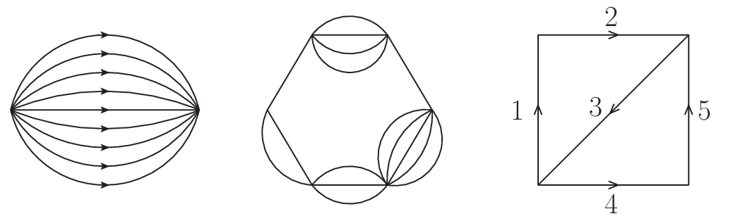
If the stack contains one or more purely virtual legs, while the other legs are Feynman propagators, no overall correction is required, as well as no corrections for subdiagrams. Combining the facts just stated, the reduction of formula (2.10) shows that the projection of the stack is just the propagator
| (7.2) |
of a single purely virtual particle with energy equal to the total incoming energy and frequency equal to the total frequency.
The bubble with “pseudodiagonal” is the stack . If all the legs are physical, its expression is the analogue of (6.3), i.e., (7.1) for a Feynman stack. If a leg is purely virtual, the reduced amplitude is (7.2).
The triangle with pseudodiagonal is the triangle where one leg is replaced by a stack . Let us assume that the first and fourth legs have the same endpoints, and their energies and have the same orientations. Then, we easily retrieve the formulas of subsection 6.2 with , .
The same works for the box with pseudodiagonal, where the endpoints of the fifth leg coincide with those of one of the first four legs. And the same works for diagrams with arbitrarily many loops: when the internal legs can be grouped together into stacks, the results coincide with those of a diagram with fewer loops, obtained by replacing each stack with a single leg, with energy equal to the total energy flowing into the stack, and frequency equal to the total frequency. An example is shown in the middle of fig. 6, which is a diagram equivalent to the hexagon. These properties hold for the Feynman diagrams, as well as for the diagrams of the reduced scattering matrices derived in section 2.
The first nontrivial arrangement at two loops is the box with (true) diagonal, shown to the right of fig. 6. The arrows are opposite to the orientations of the external energies . From [5], the threshold decomposition reads
| (7.3) | |||||
where
and , being the skeleton (6.8) of the purely virtual triangle with legs . Moreover, , and are the same as , and , respectively, with and . The sums are over the permutations of , the permutations of , plus .
We start from the case where every internal leg is quantized as purely virtual. If we apply formula (2.16) with , we find
| (7.4) |
which is the expected result, , plus a term that can be canceled by means of an overall anti-Hermitian correction. In the end, we obtain
| (7.5) |
as desired.
The reason why it is necessary to include the correction just mentioned is easily explained. Although is a prime diagram, it factorizes when we “contract” the diagonal. The contraction operation, denoted by , is studied in detail in section 8. It amounts to multiplying the skeleton diagram by and taking the limit .
Diagrammatically, the result of the contraction is a purely virtual double bubble, which is obviously not prime. We know from section 6 that such a diagram needs the correction (6.6). A consistency check is to multiply the square bracket of (7.4) by , take the limit , and verify that what we obtain is indeed canceled by the analogue of (6.6).
Now we consider the physical box with a purely virtual diagonal, i.e., the case where the diagonal is the only purely virtual leg. This time, the contraction gives the physical double bubble, which does not need any correction. Indeed, formula (2.16) at correctly gives
where means the expression (7.3) upon suppression of all the terms where any frequency , , appears in the argument of some delta function. No corrections for subdiagrams are involved, since the subdiagrams in question are triangles.
When the legs 1 and 3 are purely virtual, while all the other ones are physical, the contraction gives, again, the purely virtual double bubble, so the same correction as for (7.4) must be included. The reduced amplitude gives
in agreement with [5].
An interesting case is the one where two adjacent non diagonal legs, say 2 and 5, are purely virtual, while the others are physical. We find the same overall correction as above, because gives the purely virtual double bubble. However, we also find some unwanted terms that cannot be subtracted by means of an overall, anti-Hermitian . Luckily, they cancel out automatically, as in the other cases analyzed so far, once we include the corrections due to the subdiagrams, as per the last two terms and of formula (4.11).
The unwanted terms are subtracted away by the diagrams where the three physical legs, which are 1, 3 and 4, are crossed by the cut. One side of the cut contains the vertex , while the other side contains the corrections (4.4) to the subdiagram made by the legs 2 and 5. At the end, we correctly find
The other cases can be treated similarly.
8 Managing pure virtuality: methods and theorems
In this section and the next one we describe methods and tricks to study the virtual and on-shell contents of the skeleton diagrams , and relate the threshold decompositions of different diagrams to one another. We can even derive the threshold decompositions of bigger diagrams from the ones of smaller diagrams in a unique way. The results allow us to gain insight into the threshold decompositions themselves and the roles of the corrections. In section 10 we recap the lessons learned through the various examples.
The two main tricks are integration and contraction, which stand for: ) integrating on the external energies, and ) sending the masses to infinity.
8.1 Integration
Using the notation (6.1) (where, we recall, we multiply every propagator by with respect to the usual definitions), a basic tool is to integrate a skeleton diagram on an independent external energy :
| (8.1) |
The virtue of this operation is that it turns the Feynman propagator, as well as the cut propagators into unity:
| (8.2) |
Moreover, it turns a purely virtual (tree) propagator into zero:
| (8.3) |
We denote the operation (8.1), applied to the internal leg , by , or . It is a useful tool to inspect the diagrams and, for example, check whether they are purely virtual or not, and quantify their virtual contents versus their on-shell contents. It is also useful, as we show in the next section, to ascend and descend among the diagrams.
If we prefer to use the standard notation (3.3), (3.5), then the operation is
where denotes the skeleton diagram with propagators (3.3), (3.5).
We can apply to one or more internal legs of a diagram . We begin by studying what happens when we integrate on all the independent external energies . Taking into account that, by definition, we are already integrating on all the internal energies of a skeleton diagram, we end up integrating on all the independent energies of the diagram. So doing, all the Feynman propagators collapse to unity.
The result of this operation is called avirtuality of the skeleton diagram and measures its “on-shellness”. If is the skeleton of an ordinary Feynman diagram with (nonderivative) vertices, its avirtuality is equal to one11 1 We recall that we are working in the notation where each nonderivative vertex is equal to 1. In the usual notation, where a vertex is equal to , denoting some coupling, we would have . Diagrams with derivative vertices can be reduced to sums of diagrams with nonderivative vertices, as explained in [5]..
The purely virtual contents of the one-loop prime diagrams considered so far were singled out by reduced amplitude of formula (2.17). Denote the skeleton diagrams associated with by . We show that the avirtuality of an arbitrary with vertices is
| (8.4) |
where is defined by the recursive relation
| (8.5) |
Formula (8.4) is proved as follows. Expand the right-hand side of equation (2.17) in powers of . The th power contains vertical cuts, and each cut is equal to
The cuts identify vertical strips. Two half planes lie at the sides, their boundaries being the first and the last cuts. We consider them as further strips. The vertices of must be distributed inside the strips in all possible ways. If we include the possibility to leave some strips empty, there are ways of doing so. However, such a possibility must be excluded.
Let denote the number of distributions where such a possibility is indeed excluded. Clearly, is equal to minus the distributions that contain empty strips. Such distributions can be distinguished according to the number of empty strips, which ranges from to . There are ways of choosing the empty strips. In each case, the vertices can be distributed in ways. This gives the recurrence relation (8.5).
Each arrangement gives a contribution equal to unity, once the operation (8.1) is applied to all the independent external energies. Expanding (2.17), we thus find formula (8.4).
We see that the avirtuality of a diagram depends only on the number of vertices, not on the type of diagram . We can easily check that vanishes for every even . The avirtualities of the first odd values of are
Let us apply formula (8.4) to the examples of the previous sections. The simplest case is the avirtuality of the purely virtual propagator (4.2), which we know to be zero by formula (8.3). This is the case .
Triangle
Now we check that the avirtuality of the triangle of purely virtual particles is indeed , using formula (6.8). To this purpose, we need the identity (B.1), proved in appendix B. We have to calculate
Particular attention has to be paid to the convergence of the integrals at infinity. Ignoring the integral over for a moment, we find
| (8.6) |
The last two integrals of this list are convergent for , and give zero. The first integral can be worked out by means of (B.1) and gives
| (8.7) |
At this point, the operation gives , as we wanted to show.
One may wonder if we can add corrections to obtain zero, instead. If not, we must infer that (8.7) and are intrinsic to the diagram.
We recall that cannot change the level 0 of the threshold decomposition, which matches the Euclidean diagram. It cannot change the odd levels of the decomposition either, because they are not anti-Hermitian. So, the first level that can be affected by is the second one. There are two possibilities to remove (8.7) by means of . One is to add something containing , plus , because the operation on it can compensate (8.7). However, the symmetries under the permutations of the internal legs, and , imply that we would have to add the whole sum
The operation on the additional terms gives contributions proportional to , which must not be there.
The second possibility is to add
This is not acceptable either, since the double singularities due to these delta functions are not present in the starting triangle diagram. A quick way to see this is by noting that differences of frequencies appear, which cannot be traded for sums of frequencies. By stability, it must be possible to express all the singularities of a skeleton diagram defined by means of the Feynman prescription in terms of sums of frequencies (see [5] for details).
We conclude that the avirtuality is an intrinsic property of the purely virtual triangle diagram.
Box
The avirtuality of the box diagram with circulating purely virtual particles is equal to zero. We can verify this result as before, from formulas (6.12) and (6.13), using the identities (B.1) and (B.5) of appendix B.
We apply to (6.13): we first integrate on , then on and finally on . We can distinguish terms with three, two and one indices equal to 1. The integral gives zero on the terms that just have one index 1, since they can be organized into the sums
where is any permutation of . These integrals are separately convergent.
Each term with two or three indices equal to 1 is separately convergent, and can be calculated by means of (B.1) and (B.5). After the operation , the result is
When we finally apply , we get zero, as we wanted to show.
Following the same guidelines, we have checked the avirtualities of the purely virtual pentagon and the purely virtual hexagon (formulas (9.1), , ), finding agreement with (8.4). The projection of the purely virtual box diagram with diagonal gives (7.4), which also satisfies . The inclusion of the correction, which leads to (7.5), does not change .
8.2 Contraction
Another useful operation is the limit of infinite masses, after multiplying by the masses themselves. The basic identities are
| (8.8) |
which select the principal-value part and kill the on-shell part, and allow us to measure the virtuality of a skeleton diagram. The operation, which we denote by , where the letter stands for “contraction” and the suffix denotes the leg that is being contracted, has other interesting virtues. The first one is that it allows us to jump from one diagram to a simpler diagram, in momentum space. Later on we show that it also allows us to jump from simpler diagrams to more complicated diagrams, once it is combined with the integration trick mentioned before.
We start from an ordinary Feynman skeleton diagram , and denote the diagram obtained by contracting the leg by . For example, if is the box and is one of its internal legs, is the triangle. If is the triangle, the bubble. If is the bubble, is the tadpole. If we contract the third leg of the diagram made by three adjacent propagators, we obtain the diagram made by two adjacent propagators. Etc. Note that a connected diagram is mapped into a connected diagram . Instead, a prime diagram can be mapped into a factorized diagram . For example, we have seen that the box with diagonal turns into the double bubble, by contraction of the diagonal leg.
The other interesting property of the operation is that it applies straightforwardly to the projected skeleton diagrams, the reduced scattering matrices, and every term of the expansion of the right-hand side of formula (2.16), including the corrections. Precisely: the contraction and the projection commute.
To prove this statement, we work on the amplitude of (2.16), starting from . Let denote the projection of the Feynman skeleton diagram , the projection of the contracted diagram , and the contraction of the projected diagram . By (8.8), sends the cut propagators of the leg to zero. This means that every cut diagram contributing to , where the leg is crossed by a cut, disappears. Thus, the surviving diagrams of are precisely the ones of . We conclude that the projection encoded in the reduced amplitude commutes with the contraction at : .
It then follows that the two operations also commute at nonzero , if is the one that gives a theory of physical and purely virtual particles. The reason is that the diagrammatics of a theory of physical and purely virtual particles, recalled at the beginning of section 6, amounts to a projection that manifestly commutes with the contraction: starting from the threshold decomposition of a Feynman diagram, it suppresses the delta functions whose arguments contain the frequencies of the purely virtual particles f. The contraction suppresses the delta functions that contain , via the second limit of (8.8). The order with which we remove the two is clearly immaterial.
These properties can be used to relate the corrections of bigger skeleton diagrams to the corrections of smaller diagrams, and check the results of the previous sections. For example, if we apply to (4.3), we find the purely virtual propagator (4.2), with . If we apply to (4.4) we find 0, since the single propagator has no . If we apply to (4.8), we find (4.3) (with , due to the different conventions for the energy flows). If we apply to the difference between (4.9) and (4.8), we correctly find (4.4) (again with ). If we apply to (4.12) we obtain (4.3) again. If we apply to (4.14), we obtain , as expected. If we apply to (4.14), we correctly obtain (4.6) with . If we apply to (5.4), we find (5.2). If we apply to (5.5), we also find (5.2). If we apply to (5.5), we correctly find the physical propagator . And so on.
In loop diagrams we switch to the notation where every propagator is multiplied by with respect to the usual definitions. The basic identities are then
It is easy to check that turns the purely virtual box skeleton (6.13) into the purely virtual triangle skeleton (6.8), and turns (6.8) into the purely virtual bubble skeleton (6.4). Similarly, turns (6.15) into (6.10) with , and turns (6.17) into (6.7), etc.
The operation preserves the threshold decomposition, by which we mean that it maps level to level , for each . For example, the decomposition (6.11) of the box diagram is sent term by term into the decomposition (6.7) of the triangle diagram, by the operation . The integration operation considered before, instead, mixes different levels (see below).
9 Ascending and descending among skeleton diagrams
Now we explain how to use the operations and to ascend and descend among the skeleton diagrams. We have already described the descent in various cases, which is rather straightforward and preserves the threshold decomposition. The operation , instead, deserves a more detailed analysis.
We start from purely virtual diagrams. They are simpler, because they just contain principal values , and no delta functions . We have already proved the descent relations
where PV is the purely virtual tadpole, which vanishes. Using the formulas of [5], we can extend these results to the hexagon and the pentagon:
where22 2 We point out two typos in [5]: the factors and in front of the pentagon and hexagon expressions reported there, formula (8.2), should be replaced by and , respectively, to match the analogous factors of the triangle and the box. Further factors and in formulas (9.1) are due to the different notation we are using here for the vertices.
| (9.1) |
We want to show that we can ascend through these skeletons by means of the sole operations , and the requirement of correct behaviors at large energies (which are the convergence conditions for the operations ).
From bubble to triangle
From triangle to box
By the symmetries mentioned above, the purely virtual box can only be a linear combination
| (9.2) |
It is obtained by listing the monomials according to the following rules (codified by the “snowflake diagrams” of ref. [5]): each index must appear at least once; if it is repeated, it must be always to the left, or always to the right; no squares or higher powers of the same can appear; the monomial cannot factorize into the product of unlinked monomials (which means: monomial factors with no index in common).
From box to pentagon
The purely virtual pentagon must be a linear combination
obtained by listing the terms with 4, 3 and 2 identical left indices. After , the second and forth terms are identical, as well as the third and fifth terms, so we can set . The requirement that the total falls faster than for large gives . Finally, the requirement PVPV gives and . At the end, we get PV, as in (9.1).
From pentagon to hexagon
Listing the terms as before, the purely virtual hexagon must be a linear combination
plus . The requirement that the total falls faster than for large gives , and . The requirement PVPV gives and . The parameter multiplies a combination that is identically zero (see [5]). Setting , we get the correct PV, as in (9.1).
9.1 Ascending through the threshold decompositions
Similarly, we can derive the threshold decompositions of bigger skeleton diagrams from those of smaller skeleton diagrams . The goal is achieved by first parametrizing the most general decompositions of . After that, the arbitrary coefficients are determined by descending to smaller diagrams in all possible ways by means of the operations and . The result is unique.
We illustrate this property by studying the chain
on Feynman skeletons, which means that we assume that all the internal legs are physical. So doing, we cover all the situations obtained by the various projections, with arbitrary combinations of physical and purely virtual internal legs.
We have already shown how to ascend through the purely virtual versions of the diagrams, which is equivalent to ascend through the zeroth levels of the threshold decompositions of the Feynman diagrams. The next task is to ascend through the other levels. We do so by writing the most general linear combinations of the allowed terms, built with and according to the rules explained above and satisfying the symmetries given earlier. Then we fix the free constants by descending with the help of the operations and . The operations relate the decompositions level by level, so there is no need to rearrange the decompositions after applying them. Instead, the operations mix different levels. This means that, after applying to a bigger skeleton , the result must be decomposed anew before comparing it to the threshold decomposition of the smaller skeleton .
From bubble to triangle
We know that the zeroth level of the threshold decomposition of the triangle skeleton diagram is . We can parametrize the most general nonzero levels as
| level 1: | ||||
| level 2: |
where and are coefficients to be determined.
From triangle to box
The zeroth level of the threshold decomposition of the box skeleton diagram was determined from the parametrization (9.2). It coincides with , given in formula (6.12). Distributing the repeated indices in all possible ways, and using the symmetries mentioned earlier, the most general nonzero levels of the decomposition can be parametrized as
where , and are the coefficients that must be determined.
It is easy to check that and , as well as and , multiply identical terms, so we can set . Next, we impose the convergence of the operations . This gives and . Third, we require that the contraction gives the threshold decomposition of the triangle skeleton. Matching the various levels, we find and .
Fourth, we require that the integration also gives the triangle. When we apply the operation , we find that it does not preserve the levels of the threshold decomposition. The easiest way to see this is that returns terms that cannot be written by means of and , because they depend on differences of frequencies rather than just sums . The corresponding singularities must cancel out, since they do not belong to the triangle skeleton. Their cancellation is achieved by means of identities like (B.4), whose right-hand sides contain remnants that correct the lower levels. Once we reorganize the decomposition properly, we can match the various levels as required. We then find and .
After these substitutions we find that and multiply trivial terms, so we can set . At the end, we obtain the correct decomposition (6.11).
10 Diagrammatic rules recap
It is useful to summarize here the various diagrammatic options we have.
) Feynman diagrams
They give the usual scattering amplitudes, collected in the matrix . The ingredients are the vertices and the propagators defined by the Feynman prescription. The rules to build the diagrams follow from the time-ordered product (3.1).
) Cutkosky-Veltman diagrams
They are not used for the scattering amplitudes of the theory, but to express the unitarity equation (1.1) as a set of diagrammatic identities. The ingredients are the same as in (), plus: the conjugate vertices, the conjugate propagators, the cut propagators. The rules to build the diagrams follow from the time-ordered product (3.1) and the optical identity (1.1). Precisely: the cut is unique; one side of the cut is built with the rules (); the other side is built with the conjugate rules; the cut is given by cut propagators.
) Minimally non time-ordered diagrams
They give the scattering amplitudes of the reduced matrix . The ingredients are the same as in (), plus the non time-ordered propagators, which coincide with the cut propagators of (). No conjugate vertices, nor conjugate propagators are involved. The instructions to assemble the diagrams are encoded in formula (2.16). The diagrams may contain arbitrary numbers of cuts. The rules () are used in between two cuts, and at the sides, while the cut propagators are non time-ordered. The anti-Hermitian matrix is determined step by step to match the amplitude of a theory of physical and purely virtual particles.
) Cut diagrams of minimally non time-ordered diagrams
They include the minimally non time-ordered diagrams of , as in (), their conjugates , and the gluing of to by means of further cuts. They are used to convert the unitarity equation (2.8) satisfied by the reduced amplitude of () into diagrammatic identities.
11 Symmetries and renormalizability
In this section we show that the projection preserves the symmetries of the theory, as well as its renormalizability, under extremely mild assumptions, which are satisfied by the minimally non time-ordered product and the new quantization principle.
The diagrammatic formulation of ref. [5] provides a particular solution to the problem considered here, i.e., map the usual amplitude , which is defined by the time-ordered product (3.1) and satisfies the (pseudo)unitarity equation (2.3), into a unitary amplitude . Since (2.16) is the most general solution to the problem, there must exist an that turns into the diagrammatics of [5]. We denote it by . In the previous sections, we have shown how to derive , by requiring that the projection of a product diagram equals the product of its projected prime factors, and that this factorization property survives the basic operations of ascent and descent through the diagrams. This ensures, in particular, that itself is diagrammatic. Its diagrams can be obtained by comparing those of [5] with those of , encoded in formula (2.10). The comparison must be done iteratively for each contribution to , as soon as it appears as an overall correction to some diagram.
Now we show how to obtain the threshold decomposition of a diagram from formula (2.16). Once we choose the physical space , we know , which is the projector onto . Let denote the physical solution . Since depends just on ( and being given), we can invert its expression and expand in terms of .
Let us do this in the particular case , where is just made of the vacuum state . Then, the projection singles out the purely virtual contents of the diagrams. Inverting the formula (2.16) of , we can write as an expansion in powers of : this is precisely the threshold decomposition of the Feynman diagrams collected in .
The levels of the decomposition are the numbers of cuts, plus the levels of the corrections. The latter are determined by comparison with what they correct, which is easier to do when they appear as overall corrections.
Lorentz invariance
The threshold decomposition of ref. [5] is not manifestly Lorentz invariant, because the skeleton diagrams are defined by ignoring the integrals on the space components of the loop momenta. It is easy to show that Lorentz invariance is recovered when those integrals are resumed.
We recall that the projection to purely virtual particles amounts to consider the threshold decomposition, and remove the contributions where some delta functions, such as , depend on the frequencies of some purely virtual particles f. This operation is Lorentz invariant (as long as it is performed consistently in all the diagrams of the theory), since it amounts to remove a certain type of singularity everywhere from Feynman diagrams. Different types of singularities do not talk to one another.
Formula (2.16) is manifestly Lorentz invariant, as long as the subspace is Lorentz invariant and the correction is . The Lorentz invariance of follows by comparison between the projection obtained here and the one of [5].
Gauge symmetry, general covariance, generalized local symmetries
The physical amplitude is manifestly invariant under such symmetries, as long as projects onto an invariant subspace . This excludes subspaces containing the Faddeev-Popov ghosts, the temporal and longitudinal components of the gauge fields, etc. A quick way to prove the preservation of the symmetries is by means of the techniques recently developed in refs. [13]. There, it was shown how to dress the elementary fields to make them manifestly gauge invariant, without altering the fundamental theory. Working with dressed fields, and recalling that they reduce to the ordinary elementary fields at the level of on-shell asymptotic states, it is evident that the operations involved in formula (2.16) are manifestly gauge invariant. As far as is concerned, we can proceed as before, by comparison with [5], and recalling that: ) the projection to purely virtual particles amounts to remove certain types of singularities everywhere from Feynman diagrams; and ) different singularities do not talk to one another.
Thus, once we assume that the physical space is invariant (e.g., it is made of physically observable particles), the projection is invariant, and the preservation of symmetries is always guaranteed, including the cancellation of anomalies to all orders by means of the Adler-Bardeen theorem [14].
The results of this paper extend to the off-shell amplitudes of gauge invariant fields defined in [13]. We also recall that a particular projection is the one that gets rid of the Faddeev-Popov ghosts, as well as the temporal and longitudinal components of the gauge fields, in gauge theories. Applying the map to that case, we recover the proof of unitarity in gauge theories given in ref. [15].
Renormalizability
The renormalizability of the projected amplitudes is manifest, whenever the unprojected amplitudes are renormalizable. Indeed, formula (2.16) tells us the reduced amplitude is equal to the usual amplitude plus terms that involve one or more cuts. A single cut is sufficient to kill the overall divergence of a diagram, since the delta function due to the cut restricts the integration domain of the overall integral to a compact subset. The subdivergences are automatically taken care of as usual. The corrections are compatible with renormalizability as long as they do not affect the zeroth levels of the threshold decomposition, as we have required.
Finally, we remark that the difference between the projected amplitude and the time-ordered one vanishes identically when the incoming energy is smaller than the mass of the lightest purely virtual particle. Indeed, the diagrams of contain at least one cut leg of type , so they can be nontrivial only if exceeds the mass. In particular, vanishes in the Euclidean region, and the renormalization of the projected theory coincides with the one of the parent Euclidean theory.
12 Conclusions
We have formulated a new quantization principle for quantum field theory, based on a special type of non time-ordered product, and shown that it gives the theories of physical and purely virtual particles.
The diagrams of the physical amplitude are built by means of the usual vertices and propagators, plus non time-ordered propagators. The instructions to assemble the diagrams are encoded in a formula that maps the standard amplitude into . If obeys the unitarity or pseudounitarity equation, the most general reduced amplitude that obeys the unitarity equation depends on an arbitrary anti-Hermitian matrix . A special , called in section 11, is determined by requiring that the projection of a product diagram is equal to the product of the projected factors, and that the factorization survives basic operations of ascent and descent through the diagrams. The idea is that the time ordering should be violated in a sort of “minimum” way, inside prime diagrams. The amplitude coincides with the amplitude of a theory of physical and purely virtual particles, as given in ref. [5].
We have worked out a number of techniques to relate different diagrams. Besides descending from bigger to smaller diagrams, it is also possible to ascend in a unique way from smaller to bigger diagrams, derive their corrections, and match the threshold decompositions level by level. We have illustrated these properties in various examples. At one loop, we have considered the ascending chain bubble triangle box pentagon hexagon. At two loops, we have focused on the first nontrivial arrangement, which is the box with diagonal. In all the cases we have considered, nontrivial corrections are present when the diagram factorizes, and when it factorizes under the contractions of some internal legs. Moreover, it is always possible to ascend through the threshold decompositions in a unique way. We conjecture that these are general properties of the physical amplitude .
Purely virtual particles provide the most elegant way to break the crystal glass of time ordering. To give the reader an idea of how inelegant the most general solution (2.16) is, consider that, when is generic (including ), a diagram with non-amputated external legs is not straightforwardly related to the same diagram with amputated external legs, and has to be calculated anew. Moreover, the usual definitions of generating functionals of connected and irreducible Green functions do not apply. Only for , we have that, if denotes the generating functional all the correlation functions, its logarithm is the generating functional of the connected ones, and the Legendre transform , , is the generating functional of the amputated, one-particle irreducible ones.
Yet, we cannot exclude that unforeseen physical principles might one day point to one of the many alternative options. In the absence of experimental data, the only thing we can do is single out the options that have remarkable formal and diagrammatic properties. In this spirit, it may be also worth to search for alternative corrections, which may break the time ordering in non minimal ways, but have other interesting properties. In any case, the right solution chosen by nature must lie somewhere in formula (2.16), determined by the that fits the physics.
We conclude with a brief summary of the formulations of purely virtual particles worked out so far. First, a nonanalytic Wick rotation was introduced in refs. [16], as a way to get rid of ghosts with complex masses, and reformulate the Lee-Wick models [17]. Its key ingredient is the average continuation around the branch cuts of amplitudes. It was soon realized that the procedure was actually a way to formulate models of new types, rather different from the original Lee-Wick idea (see [18] for a detailed comparison), and could be extended to remove ghosts with real masses (as well as physical particles), to give sense of quantum gravity as a power counting renormalizable theory, like the standard model [6]. The proof of unitarity to all orders in this approach was given in ref. [18]33 3 For Lee-Wick approaches to quantum gravity, we address the reader to refs. [19]. Among other approaches to the problem of removing ghosts in quantum field theory, we point out [20]..
The second, equivalent formulation of purely virtual particles was introduced by means of the diagrammatic threshold decomposition of [5], and the spectral optical identities derived from it. The third formulation, equivalent to the other two, is the one of the present paper, based on the minimally non time-ordered product. With respect to [18], the gain offered by the two new formulations is considerable, not only for the clarity of the proofs to all orders, but also from the practical point of view. Indeed, the new formulations offer several ways to make calculations with not much more effort than computing Feynman diagrams (check [8]).
We end by mentioning some perspectives for the future. One goal is to develop the operatorial/Hamiltonian approach to purely virtual particles, and maybe study their quantum mechanics, where the evolution operator is no longer the usual time-ordered exponential, but follows from the minimally non time-ordered product. Another challenging objective is to pursue the off-shell formulation of transition amplitudes, by combining the approach of this paper with the results recently obtained in refs. [13], where it was shown how to define off-shell physical amplitudes of colored states in QCD and point-dependent observables in quantum gravity, consistently with the (off-shell version of the) optical theorem.
All in all, we think that we have achieved a satisfactory understanding of the nature of purely virtual particles, and revealed the main mysteries behind them, in view of the challenges just mentioned.
Appendices
A From diagrams to scattering matrix, and back
Although the matrix is a collection of diagrams, in the paper we have been able to concentrate on single diagrams, and isolate the identities satisfied by them. In this appendix we show how to switch from to single diagrams, with a different particle in each internal leg (and vice versa), with no loss and no gain of information.
For definiteness, we start from a Lagrangian that depends on a single field . We separate the kinetic (i.e., quadratic) part , where denotes the mass of , from the interaction part (made by anything that is not quadratic in , including the linear terms, if present), where denotes the couplings:
| (A.1) |
Then we use a Pauli-Villars trick [12] to introduce many fields without changing the diagrams. Specifically, we replace the kinetic part with the sum of the kinetic parts, having the same mass. Moreover, we replace with the sum of all the in the interaction part:
| (A.2) |
The diagrams with external legs, generated by this Lagrangian, coincide with those generated by (A.1), multiplied by and an appropriate combinatorial factor. To prove this, it is sufficient to note that each internal leg carries the propagator, which is the sum of the propagators, which in turn is equal to the propagator. We can choose the external legs we want, and the diagram is always the same, apart from the factors in front.
At this point, we give a different mass to each field , and a different coupling to each vertex obtained by expanding the interaction part, where the subscript refers to the various possibilities we have. We obtain
for a certain, new interaction Lagrangian . We know that we retrieve the diagrams of the starting theory when we set all the masses equal to , and all the couplings equal to the appropriate values .
Now we show that the extended Lagrangian allows us to isolate the diagrams as needed. Let and denote the usual (unprojected) amplitudes, associated with and , respectively. Let and denote diagrams contributing to them. For any there exists a generalization with the same topology as , where each internal leg propagates a different field . It is sufficient to take sufficiently large, to have a sufficient number of different fields , and differentiate with respect to suitable couplings . After that, we set for every .
After building the diagram with this method, we can study the diagrammatic identities satisfied by it, and build the projections we need, by differentiating formula (2.16) with respect to the appropriate couplings. If the corrections are determined as explained in the paper, the right identities are obtained by differentiating (2.16) at as well.
An advantage of is that its combinatorics are trivial, since there is only one Wick contraction for each field participating in it. When we set the masses equal to one another, and identify the couplings appropriately to go back to the original theory (A.1)-(A.2), several diagrams give identical contributions and restore the right combinatorics of .
In the paper, we built diagrams with independent internal legs and no external legs, replaced by external sources . The sources can be replaced by products of physical fields without affecting the results we have obtained, as long as the external legs are amputated. When we need to include propagators on the external legs, we can use the factorization property, since we know that the right gives the factorized result. With a generic , instead, the factorization property does not hold and we must redo the whole projection.
B Identities for product distributions
In this appendix we prove some identities for product distributions that we have used in the paper. The first one is
| (B.1) |
where is real. It be proved by integrating the expression
on from to . Since the integral of the terms in square brackets gives zero, we obtain
| (B.2) |
Formula (B.1) then follows by using
| (B.3) |
twice inside the integral (B.2). Below, we reassure the reader that it is correct to use the decomposition (B.3) in products.
More quickly, formula (B.1) can be also proved from the identity
| (B.4) |
derived in ref. [5]. The integral of the left term is convergent and gives zero, so the rest gives (B.1).
The second identity we need is
| (B.5) |
We start from the formula
which was derived again in ref. [5]. First, we reflect to , then translate and by , finally rescale by a factor 2. Integrating on , we get
Every integral is separately convergent, so using (B.1) we obtain (B.5).
Now we show that it is correct to use the decomposition (B.3) in products. Consider
where is a generic test function in two variables and the integral is over the plane , with measure . Decompose as the sum of
according to the and parities, where and can be or . Note that
since is regular for and . Moreover,
and
Thus,
References
- [1] R.E. Cutkosky, Singularities and discontinuities of Feynman amplitudes, J. Math. Phys. 1 (1960) 429.
- [2] M. Veltman, Unitarity and causality in a renormalizable field theory with unstable particles, Physica 29 (1963) 186.
- [3] G. ’t Hooft, Renormalization of massless Yang-Mills fields, Nucl. Phys. B 33 (1971) 173; G. ’t Hooft, Renormalizable Lagrangians for massive Yang-Mills fields, Nucl. Phys. B 35 (1971) 167.
- [4] G. ’t Hooft and M. Veltman, Diagrammar, CERN report CERN-73-09; M. Veltman, Diagrammatica. The path to Feynman rules (Cambridge University Press, New York, 1994).
- [5] D. Anselmi, Diagrammar of physical and fake particles and spectral optical theorem, J. High Energy Phys. 11 (2021) 030, 21A5 Renorm and arXiv: 2109.06889 [hep-th].
- [6] D. Anselmi, On the quantum field theory of the gravitational interactions, J. High Energy Phys. 06 (2017) 086, 17A3 Renorm and arXiv: 1704.07728 [hep-th].
- [7] D. Anselmi, E. Bianchi and M. Piva, Predictions of quantum gravity in inflationary cosmology: effects of the Weyl-squared term, J. High Energy Phys. 07 (2020) 211, 20A2 Renorm and arXiv:2005.10293 [hep-th].
- [8] A. Melis and M. Piva, One-loop integrals for purely virtual particles, arXiv:2209.05547 [hep-ph].
- [9] G. J. van Oldenborgh and J. A. M. Vermaseren, New Algorithms for One Loop Integrals, Z. Phys. C 46 (1990) 425. J. Kublbeck, M. Bohm, and A. Denner, Feyn Arts: Computer Algebraic Generation of Feynman Graphs and Amplitudes, Comput. Phys. Commun. 60 (1990) 165; A. Denner, Techniques for calculation of electroweak radiative corrections at the one loop level and results for W physics at LEP-200, Fortsch. Phys. 41 (1993) 307 and arXiv:0709.1075; T. Hahn, Loop calculations with FeynArts, FormCalc, and LoopTools, Acta Phys. Polon. B30 (1999) 3469 and arXiv:hep-ph/9910227; T. Hahn, Generating Feynman diagrams and amplitudes with FeynArts 3, Comput. Phys. Commun. 140 (2001) 418 and arXiv:hep-ph/0012260; A. Alloul, N. D. Christensen, C. Degrande, C. Duhr and B. Fuks, FeynRules 2.0 - A complete toolbox for tree-level phenomenology, Comput. Phys. Commun. 185 (2014) 2250 and arXiv:1310.1921; H.H. Patel, Package-X: A Mathematica package for the analytic calculation of one-loop integrals, Comput. Phys. Commun. 197 (2015) 276 and arXiv:1503.01469 [hep-ph].
- [10] K.N. Abazajian et al., CMB-S4 Science Book, First Edition, arXiv:1610.02743 [astro-ph.CO].
- [11] D. Anselmi, K. Kannike, C. Marzo, L. Marzola, A. Melis, K. Müürsepp, M. Piva and M. Raidal, A fake doublet solution to the muon anomalous magnetic moment, Phys. Rev. D 104 (2021) 035009, 21A4 Renorm and arXiv:2104.03249 [hep-ph].
- [12] W. Pauli and F. Villars, On the invariant regularization in relativistic quantum theory. Rev. Mod. Phys. 21 (1949) 434.
- [13] D. Anselmi, Purely virtual extension of quantum field theory for gauge invariant fields: Yang-Mills theory, 22A3 Renorm and arXiv:2207.11271 [hep-ph]; D. Anselmi, Purely virtual extension of quantum field theory for gauge invariant fields: quantum gravity, 22A4 Renorm and arXiv:2207.12401 [hep-th].
- [14] S.L. Adler and W.A. Bardeen, Absence of higher order corrections in the anomalous axial vector divergence, Phys. Rev. 182 (1969) 1517; for a review and references, see also S.L. Adler, Anomalies to all orders, in “Fifty Years of Yang-Mills Theory”, G. ’t Hooft ed., World Scientific, Singapore, 2005, p. 187-228, and arXiv:hep-th/0405040; for a textbook, see M.E. Peskin and D.V. Schroeder, An introduction to quantum field theory, Westview Press, Boulder, Colorado, 1995, Chapter 20.
- [15] D. Anselmi, Fakeons, unitarity, massive gravitons and the cosmological constant, J. High Energy Phys. 12 (2019) 027, 19A2 Renorm and arXiv:1909.04955 [hep-th].
- [16] D. Anselmi and M. Piva, A new formulation of Lee-Wick quantum field theory, J. High Energy Phys. 06 (2017) 066, 17A1 Renorm and arXiv:1703.04584 [hep-th].
- [17] T.D. Lee and G.C. Wick, Negative metric and the unitarity of the S-matrix, Nucl. Phys. B 9 (1969) 209; T.D. Lee and G.C. Wick, Finite theory of quantum electrodynamics, Phys. Rev. D 2 (1970) 1033. R.E. Cutkosky, P.V Landshoff, D.I. Olive, J.C. Polkinghorne, A non-analytic S matrix, Nucl. Phys. B12 (1969) 281; T.D. Lee, A relativistic complex pole model with indefinite metric, in Quanta: Essays in Theoretical Physics Dedicated to Gregor Wentzel (Chicago University Press, Chicago, 1970), p. 260. N. Nakanishi, Lorentz noninvariance of the complex-ghost relativistic field theory, Phys. Rev. D 3 (1971) 811; B. Grinstein, D. O’Connell and M.B. Wise, Causality as an emergent macroscopic phenomenon: The Lee-Wick O(N) model, Phys. Rev. D 79 (2009) 105019 and arXiv:0805.2156 [hep-th].
- [18] D. Anselmi, Fakeons and Lee-Wick models, J. High Energy Phys. 02 (2018) 141, 18A1 Renorm and arXiv:1801.00915 [hep-th].
- [19] E. Tomboulis, 1/N expansion and renormalization in quantum gravity, Phys. Lett. B 70 (1977) 361; E. Tomboulis, Renormalizability and asymptotic freedom in quantum gravity, Phys. Lett. B 97 (1980) 77; Shapiro and L. Modesto, Superrenormalizable quantum gravity with complex ghosts, Phys. Lett. B755 (2016) 279-284 and arXiv:1512.07600 [hep-th]; L. Modesto, Super-renormalizable or finite Lee–Wick quantum gravity, Nucl. Phys. B909 (2016) 584 and arXiv:1602.02421 [hep-th]; J.F. Donoghue and G. Menezes, Unitarity, stability and loops of unstable ghosts, Phys. Rev. D 100 (2019) 105006 and arXiv:1908.02416 [hep-th].
- [20] C.M. Berends and P.D. Manheim, No-ghost theorem for the fourth-order derivative Pais-Uhlenbeck oscillator model, Phys. Rev. Lett. 100 (2008) 110402 and arXiv: 0706.0207 [hep-th].