Cell dynamics in microfluidic devices under heterogeneous chemotaxis and growth conditions: a mathematical study
Abstract
As motivated by studies of cellular motility driven by spatiotemporal chemotactic gradients in microdevices, we develop a framework for constructing approximate analytical solutions for the location, speed and cellular densities for cell chemotaxis waves in heterogeneous fields of chemoattractant from the underlying partial differential equation models. In particular, such chemotactic waves are not in general translationally invariant travelling waves, but possess a spatial variation that evolves in time, and may even may oscillate back and forth in time, according to the details of the chemotactic gradients. The analytical framework exploits the observation that unbiased cellular diffusive flux is typically small compared to chemotactic fluxes and is first developed and validated for a range of exemplar scenarios. The framework is subsequently applied to more complex models considering the full dynamics of the chemoattractant and how this may be driven and controlled within a microdevice by considering a range of boundary conditions. In particular, even though solutions cannot be constructed in all cases, a wide variety of scenarios can be considered analytically, firstly providing global insight into the important mechanisms and features of cell motility in complex spatiotemporal fields of chemoattractant. Such analytical solutions also provide a means of rapid evaluation of model predictions, with the prospect of application in computationally demanding investigations relating theoretical models and experimental observation, such as Bayesian parameter estimation.
1 Introduction
Most biological processes integrate different cell populations, extracellular matrix (ECM) properties, chemotactic gradients and physical cues, constituting a complex, dynamic and interactive microenvironment [1, 2, 3, 4, 5]. Cells are also constantly adjusting to accommodate their surroundings, particularly for homeostatically maintaining the intracellular and extracellular environment within physiological constraints [6]. In response to the different chemical and physical external stimuli, cells can modify their shape, location, internal structure and genomic expression, as well as their capacity to proliferate, migrate, differentiate, produce ECM or other biochemical substances, changing, in turn, the surrounding medium as well as sending new signals to other cells [7, 8, 9]. This two-way interaction between cells and their environment is crucial in physiological processes such as embryogenesis, organ development, homeostasis, repair, and long-term evolution of tissues and organs among others, as well as in pathological processes such as atherosclerosis or cancer [10, 11, 12, 13]. Furthermore, developing novel frameworks to investigate and elucidate these mechanisms and interactions is key to developing novel therapeutic strategies aiming at promoting (blocking) desirable (undesirable) cellular behaviours [14].
In particular, due to the underlying complexity, in vivo research – both in humans and in animals – is impeded by the fact it is difficult to control and isolate effects. Thus, a simpler alternative is using in vitro experiments. Nevertheless, the predictive power currently available, whether in vivo or in vitro, is still poor, as demonstrated the continuous drop in the number of new drugs appearing annually, despite billion-dollar investments [15, 16]. Indeed, structural three-dimensionality is one of the most important characteristics of biological processes [17], but in vitro cells are mostly cultured in a traditional Petri dish (2D culture), where cell behaviour is dramatically different from real tissues [18]. Recently, microfluidics has arisen as a powerful tool to recreate the complex microenvironment that governs tumour dynamics [19, 20]. This technique allows the reproduction of numerous important features that are lost in 2D cultures, as well as testing drugs in a much more reliable and efficient way [21, 22, 23, 24, 25].
In addition to such in vitro models, mathematical in silico models are a powerful tool for dealing with many problems in physics, engineering, and biology. In particular, cell population evolution models based on transport partial differential equations (PDEs) have been widely used to study many biological processes, including cancer [26, 27]. For instance, tumour development is a key example of a highly dynamic and complex biological process that originates from external signals or stimuli modulated by the particular microenvironment. Furthermore, when a given treatment is applied (surgery, chemotherapy, radiotherapy, immunotherapy, hormones or a combination thereof), the tumour and its microenvironment undergo significant alterations. This leads tumour cells to proliferate and generate microenvironments that promote the death of surrounding cell types and the survival of tumour cells that are more adaptable and resistant. That is why, when modelling the enormous variety and complexity of a tumour and its microenvironment, the resulting differential equations are highly non-linear and strongly coupled [28, 29, 30]. The numerical resolution of the equations, especially in the era of high performance computing, has been extensively utilised in the simulation of “what if” scenarios and the study of effects and hypotheses in isolation, something that is often impossible to do with in vivo and in vitro models [31, 32]. In turn, the construction and exploitation of in silico experiments is thus being increasingly used in the early stages of designing drugs and therapies against tumours.
A particular niche of interest is Glioblastoma (GBM), the most common and aggressive primary brain tumour [33], with extensive studies dedicated to mathematical modelling its evolution [34], reproducing aspects of GBM histopathology [29] and incorporating the influence of tumour microenvironment (TME) chemical and mechanical cues [35]. It has been demonstrated that GBM progression is extensively controlled by the local oxygen concentrations and gradients [36], motivating many studies to incorporate the role of oxygen gradients and hypoxia in tumour progression [37, 38, 39]. Some models of GBM have reproduced cell culture evolution under different experimental configurations [40], using a go-or-grow transition switch, governed by nonlinear activation functions for the chemotaxis and growth. Such studies therefore implicate the balance between cell migratory and proliferative activity, together with their relation to the different TME stimuli, as playing a key role in GBM evolution.
Nevertheless, the complexity of the equations to be solved often require numerical simulations that are impractical, due to the high computational cost, especially in the resolution of inverse problems such as parameter estimation, model selection, the design of experiments, sensitivity studies, model structural analysis and Uncertainty Quantification (UQ). Although many modern techniques as Reduced Order Models (ROM) and metamodels using Artificial Intelligence (AI) have been developed in recent years [41], the existence of analytical solutions, although approximate, provides key information to test and validate numerical algorithms, inform a mechanism based understanding across parameter space and to allow initial predictions of Quantities of Interest (QoI), such as travelling fronts, equilibria, the ranges of variation in the solution across parameter space and parameter sensitivities, among others. Indeed, some works in the last years have focused on the use of these techniques for analysing GBM progression [42, 43, 44].
The interaction of cells with a chemoattractant leads to a type of Keller - Segel (K-S) model [45], which generally have a rich structure as reviewed by G. Arumugam and J. Tyagi [46]. One of the main interests concerning the K-S model is the existence and characteristics of travelling waves (see for instance [47]). In this work, we explore the dynamics of cell populations under gradients of a chemotactic agent for one-dimensional problems. We move beyond travelling waves to investigate evolving wave solutions in the heterogeneous environments that are often found in microdevices and physiology. This general class of problems allows the treatment of a wide variety of situations related to the evolution of tumours, while the analysis of the associated PDEs enables the quantification of histopathological characteristics, such as the spread of pseudopalisades and the response of the population to oscillatory stimuli. This knowledge can be used for the design of experiments, to speed up the characterisation processes of cell populations and to validate or rule out possible models.
In particular, we are interested in modelling cell motility dynamics in microfluidic devices, which are experimental platforms that have been demonstrated to accurately recreate biomimetic physiological conditions [48], with application in bioengineering and biomedical research [19]. In many situations, the chemotactic agent concentration may be assumed as known, either because it can be directly measured, or because its concentration can be computed by solving a diffusion problem that is, to good approximation, decoupled from the cell population field.
To proceed, we first describe the structure of the mathematical problem associated with the response of cell populations to chemotactic gradients, together with the general assumptions and hypotheses about the underlying mechanisms. We derive pertinent features about the solution field, for instance that it possesses a migratory structure with a transition zone wavefront. We are also able to estimate the wave front evolution and the shape of the solution profile. In particular, we compute an analytical solution for specific exemplar cases associated with specific relevant experimental situations. These include a constant spatial gradient of chemoattractant, together with temporal oscillations associated with a fluctuating source, quadratic profiles of chemoattractant, offering additional nonlinear features, and an exponential profile of chemoattractants corresponding to the diffusion from a localised source. We further apply the general results to the analysis of a cell culture microfluidic experiment, representing a slightly simplified version for an in vitro model of GBM progression, as developed in [40], showing how the methods presented here can generate analytical results for the simulation of microdevice representations for migratory tumour cell dynamics.
2 Methods
2.1 The model
We study a broad class of problems that are related to the dynamics of a cell culture in microfluidic devices under the influence of a chemotattractant, when the concentration of the agent can be computed or measured. A schematic view of this situation is represented in Fig. 1.


The non-dimensional equation for the cell population concentration, , represents cellular diffusion and chemotaxis in response to a heterogeneous field of chemoattractant that generates an advective flux , and also impacts cellular proliferation via so as to generate the governing equation
| (1) |
with the non-dimensional cellular diffusion coefficient. This governing equation is also supplemented by zero-flux boundary conditions, given by
| (2a) | ||||
| (2b) | ||||
and initial conditions
| (3) |
2.2 Computation of the general solution for small diffusion
2.2.1 Outer solution
The main hypothesis, which is usually true for cellular motility due to weak cell-based random motility, is that the non-dimensional diffusion coefficient satisfies , as we will verify below in the case of GBM cells in microdevices. Hence, away from boundary layers, diffusion may be neglected compared to the influence of growth and chemoattractant driven migration. Then, Eq. (1) may be approximated by:
| (4) |
This is a first-order hyperbolic PDE, amenable to the method of characteristics. If we know the initial data , we can parameterise the initial data via with the relation . Also, there is another family of characteristic curves, emerging from the points where and , with the imposition of the boundary condition of no flux, Eq. (2). Assuming that , and that the boundary is away from the transition region of the cellular wavefront, so that to excellent approximation since spatial gradients are small, we conclude from the boundary contition, Eq. (2), that to the same level of approximation. Therefore, this boundary condition can be parameterised via with the relation . Hence, at and there is an emerging singular characteristic that splits the domain in two regions. The geometric interpretation of the method of characteristics is shown in Fig. 2, which shows the projection of the characteristic curves onto the plane .
We have, therefore, two families of characteristic curves. For the first one:
| (5a) | ||||
| (5b) | ||||
| (5c) | ||||
and for the second:
| (6a) | ||||
| (6b) | ||||
| (6c) | ||||
Noting the uniqueness of the solution to Eqs. (6) courtesy of Picard’s theorem, we have by inspection that these equations only generate the trivial solution .
However, the solution to the first family, given by Eqs. (5), is typically more complex, though one always has
| (7) |
Progress can be readily made when
- •
is linear in , such that
- •
is separable, that is .
In particular when is linear in we have
| (8) |
which defines for . We generalise this definition so that on the characteristic curve given by the value of , and whenever this relation can be uniquely inverted for , we write .
In contrast when Eqs. (5a) and (5b) may be integrated to obtain
| (9) |
In turn, Eq. (9) generates the relation on the characteristic curve. Further motivation for examples of linear and separable chemotactic response functions for are given in Section 3 below.
In both cases, or even in the more general case where cannot readily be determined analytically for all relevant , the location of the transition from , and thus the location of the transition region for the cellular wavefront, , is given by the characteristic with – hence . This is particularly informative about the general behaviour of the solution, for instance in determining the wavespeed. With respect to Eq. (5c), we proceed using the change of variable , we obtain the ODE in terms of the variable:
| (10) |
where for the linear case and for the separable case.
Noting the integration is along a characteristic, and thus is fixed, this equation is of the form for and , with fixed, so a general expression is given by
| (11) |
where is indeed the value of at the location of the characteristic when .
Recapping, suppose may be inverted to give . Then, noting
by the parameterisation of the initial data, we have
and, in particular
Combining these expressions with Eq. (11), we obtain a general expression for and therefore for :
| (12) |
where is fixed on each characteristic curve and
Eq. (12) may be also written in terms of and directly, obtaining
| (13) |
A special separable case for
Often below, when the chemoattractant flux term is independent of time, so that , we will have , , . In these circumstances we have the simplification
by the symmetry in Eq. (9) with and also that
which gives
Recalling that the integration is along a characteristic, so that is fixed, we change the integration variable via , noting from Eq. (7) and from Eq. (5b), with fixed and , that
Hence, on further noting and , we have, to within corrections, that
| (14) |
In the examples plotted below we also have is constant, in which case collapses to the constant . For clarity please note that is an abbreviation for in general, though this is constant and denoted simply by in all examples, separable or otherwise, plotted below.
2.2.2 Inner solution
To explore the transition layer moving with the wavefront, we introduce a scaling of coordinates such that diffusion and advection provide a leading order dominant balance in the transition layer, with for the inner variable and . With the change of variables
one has the inner solution equations
where the second line uses . We take to bring the advective and diffusive terms into a nominal dominant balance.
Let us now assume that uniformly possesses an order one derivative with respect to , that is, we assume that , therefore
for . The solution of this equation, when , with the Heaviside step function is
2.2.3 Composite solution
We can combine the inner solution, rewritten in terms of with the outer solutions via a composite approximation to generate an approximation for the full numerical solution across the domain (away from any prospective boundary layer at ). Thus, with , constant, and the analytical characteristic solution of Eq (13) we have
| (15) |
so, finally:
| (16) |
For the special case discussed in the previous section, that is, when , and , and in particular so that for this special case
| (17) |
with continuity assured from the constraint , which holds as, by construction, both and on the separating characteristic and .
2.3 Some particular cases of interest
The solution given by Eq. (13) is general given that , though even in the separable case using Eq. (9) to determine the functions and can generate complicated solutions that are not readily expressed in terms of standard functions. Further, even when is separable or linear, allowing extensive analytical progress, there is still considerable freedom in the form of and hence we firstly analyse models where is linear, quadratic, and exponential in space, before proceeding to consider an example of cellular behaviour in a microdevice.

2.3.1 Linear chemotaxis
We first consider a function of the form
| (18) |
Hence, the transition is located at
| (21) |
Furthermore, for and , so that , the integral expression for in Eq. (13) is readily determined to reveal
while before the transition. Fig. 3 shows a comparison between the numerical results with and the approximate analytical solution for and . For this plot, and for analogous plots below, note the accurate prediction of the evolving front, and the general agreement between the numerical and analytical solutions for . Furthermore, one can expect boundary layer effects near the right hand edge of the domain, , that are not captured by the presented solution, though these are not plotted in the current Figure.
A further, and particularly relevant case, is when , whence
| (22a) | ||||
| (22b) | ||||
Note we still have since is even so that remains a symmetry of Eq. (9). The transition is located at
| (23) |
Fig. 4 shows the comparison between the numerical results with and the analytical solution, with . Note that as all the domain is displayed, the boundary layer in the numerical solution near can be readily observed.

The oscillating gradient case is very pertinent as it corresponds to the case where the oxygenation feed between the two channels at the microfluidic device switches, so we shall explore it in more detail. Rather than working with the general solution given by Eq. (13) it can be more expedient to consider the differential equation for given by Eq. (10); noting , , , constant, for the cases considered here, this reduces to
| (24) |
with no -dependence. Hence, on the right of the transition region the solution is constant, .
In Appendix A we show that Eq. 24 may be solved using different asymptotic methods for four different regimes:
- •
Slow variations of the gradients, .
- •
Fast variations of the gradients, .
- •
Dominant chemotaxis, .
- •
Dominant growth, .
For spatial locations to the right of the transition region, but away from any boundary layer at , these approximate solutions are compared to numerical solutions computed using standard Runge-Kutta solvers in Fig 5.


2.3.2 Quadratic chemotaxis
Now, we consider a function of the form
| (25) |
and hence .
- •
If , Eq. (9) gives
(26) and in turn
(27a) (27b) The transition is located at
(28) Furthermore, in the case where we have to an accuracy of that
via use of Eq. (14), with where significant, but elementary, manipulation is required to deduce the final expression. In particular for the parameters of Fig. 6(a) it is straightforward to show that at leading order the behaviour in for fixed is linear, as observed in this figure.
- •
Furthermore, the analytical and full numeric solutions are plotted for the parameters with in Fig. 6(b). For this set of parameters, where as in Fig. 6(b), we have
(32) Dropping the corrections in higher powers of , valid for sufficiently small time including the times plotted in Fig. 6, we have
and then also dropping terms scaling with , one finds
with a relative correction of The latter again gives an approximate linear dependence in for fixed given the parameters of Fig. 6(b), as observed.
- •
If , Eq. (9) gives
(33) so that
(34a) (34b) where we have defined and , with the transition location given by
(35) For Fig 6(c), we again have , so that ; we also have throughout the simulation regime. Hence, on neglecting higher powers of , the transition location simplifies to
which agrees with the above as Furthermore, under these conditions with and neglecting higher orders in , one finds
with an relative error of For fixed, again we have is approximately linearly decreasing in , as observed in Fig 6(c).


More generally, Fig. 6 shows a comparison between the numerical results with , and the analytical solution for three different expressions of and , with full consistency with the above solutions and approximations.

2.3.3 Exponential chemotaxis
We consider now a function of the type:
| (36) |
Then, we have , with Eq. (9) reducing to
| (37) |
Hence
| (38a) | ||||
| (38b) | ||||
with the transition is located at
| (39) |
In particular, if this reduces to
| (40a) | ||||
| (40b) | ||||
and
| (41) |
Fig. 7 shows the comparison between the numerical results and the analytical solution with and , . Furthermore, in this regime on neglecting corrections, we have
noting that on this characteristic, so that
in turn demonstrating that does not possess a singularity with exponential decay in for fixed away from the transition to a good approximation, as may be also observed in Fig. 7.
3 Applications to microfluidic experiments
3.1 The general model
We study a broad class of problems that are related to the evolution of a cell culture in microfluidic devices under a chemotactic agent, such as oxygen, when the concentration of the agent can be computed or measured, as schematically represented in Fig. 1. Hence we proceed to consider the following model of generic cell culture evolution in microfluidic devices:
| (42a) | ||||
| (42b) | ||||
| (42c) | ||||
where and are respectively the alive and dead cell concentrations and is a chemotactic agent, and are nonlinear dimensionless corrections accounting for the effect of the chemo-attractant on cell growth and death. In addition is the nonlinear dimensionless correction of the chemo-attractant consumption by all cells in the microdevice, noting that additional cells other than those of direct interest may be present, such as the study of metastatic tumour cells of interest migrating within a stromal cell population for instance. We also assume that dead cell concentration is sufficiently low that it does not compromise either live cell proliferation or migration. Note that if the chemotaxis agent is a cell nutrient, such as glucose or oxygen, , whereas for unconsumed biochemical signals, . The boundary conditions considered are
| (43a) | ||||
| (43b) | ||||
| (43c) | ||||
| (43d) | ||||
with and , the chemotactic agent concentration at the left and right channel, and the alive cell flow. As the dead cell population is slave to the other variables in this model, we neglect it henceforth which is equivalent to taking .
Therefore, the full model here analysed is
| (44a) | ||||
| (44b) | ||||
In order to evaluate the relevance of the different phenomena, we define the dimensionless variables:
| (45a) | ||||
| (45b) | ||||
| (45c) | ||||
| (45d) | ||||
Hence Eqs. (44) become
| (46a) | ||||
| (46b) | ||||
where
| (47a) | ||||
| (47b) | ||||
| (47c) | ||||
| (47d) | ||||
| (47e) | ||||
| (47f) | ||||
The associated boundary conditions are
| (48a) | ||||
| (48b) | ||||
| (48c) | ||||
| (48d) | ||||
where now and are prescribed functions of time corresponding to the level of nutrient or chemoattractant fixed to be at the channel edges. In what follows, we will use and as an abbreviation for and .
In particular the governing PDEs described in Eqs. (46) may be reformulated as
| (49a) | ||||
| (49b) | ||||
3.1.1 The weak consumption limit
First we consider the case where the chemoattractant is not a nutrient and therefore is not consumed by cells. In that case, we can set
For all the problems in which it is possible to assume , whereby random cellular motility is negligible compared to directed chemotaxis and with , so that the chemoattractant diffusion is large relative to cellular diffusion Eqs. (49) reduce to
| (50a) | ||||
| (50b) | ||||
where .
However, care is required in considering the boundary conditions for and the initial conditions for in this reduced model, due to the loss of the second spatial derivative of and the first temporal derivative of . In particular, we cannot satisfy all the boundary conditions for ; instead we have boundary layers. We have seen in the examples these occur at internal transitions and at the right of the domain (see Fig 4). Thus for the simplified system the boundary condition is enforced at for with the simplification of the flux to , as diffusion is treated as negligible. However, enforcing the boundary condition at will require the consideration of a boundary layer that is not resolved in the simplified model as it is complicated, but does not further insight into cell migratory and chemotaxis. The two boundary conditions for , as given by Eqs. 48c and 48d are inherited and applied at both boundaries. We now consider the initial conditions for , which cannot be satisfied. Instead there is an analogous temporal boundary layer for early time while initial transients relax, though such transients persist for such a short time that they are not of interest, and thus not resolved, here. The justification of the neglect of these fast transients is further detailed in Appendix B, where it is demonstrated that the solution of Eqn (50b) corresponds to the leading order composite solution in a temporal boundary layer analysis that exploits .
Proceeding, we set and , Eq. (50b) is immediately integrated to
| (51) |
We recover therefore Eq. (4) with
that is a special case of the linear problem , with and , so the different functions needed in order to compute the solution are:
| (52a) | ||||
| (52b) | ||||
| (52c) | ||||
where we have defined . Also, the expression of the cell profile far from the transition is
| (53) |
where
| (54) |
The evolution of the transition coordinate and the dimensionless cell profile for different times are shown in Fig. 8 for , and different external stimuli . In particular, let us consider the case with , and with and use of the change of variable , whereby on a characteristic
with and . This reveals
Combined with Eq. (53), this gives a simple expression for . For instance
for constant; in this case, we have an increasing function at fixed to the right of the transition given and this is essentially linear for , as observed in Fig. 8.


3.1.2 Cellular consumption of chemoattractant
A more interesting case is when the chemoattractant is a nutrient and therefore it is consumed by cells. In that case, .
With denoting the non-dimensional uptake of nutrient per cell, we take to be monotonic increasing with
| (55a) | |||
| (55b) | |||
where the final limit is without loss of generality, with the overall scale of uptake governed by .
For instance, with Michaelis-Menten kinetics we take [49]:
| (56) |
or, more in general, Hill-Langmuir equation for modelling the consumption kinetics [50]
| (57) |
In any of the aforementioned cases, there are numerous potential scenarios:
- 1.
There are no other cells at the microfluidic device besides the cell culture of our interest and we are at the low cell regime, . In that case, after rapid initial transients describing the diffusion relaxation of the nutrient, and too fast to be on the timescale of cellular motility, Eq. (49b) becomes , and the discussion is analogous to the case without the consumption term.
- 2.
There are other non-migrating cells within the microfluidic device in addition to the migrating cells, for instance if we are considering a metastasis model, with the other cells at constant concentration and in excess of the tumour cells. If we additionally have high nutrient concentrations the situation is illustrated in Fig. 9(a) using oxygen as an example of nutrient. In that case, and have
where is the (dimensionless) total amount of cells, essentially constant as the non-tumour cells are in excess. Then, with the definition
Eq. (49b) becomes
(58) In addition, we assume so that may be treated as order one on using asymptotic methods based on on the leading order of approximations based on . Then the above further reduces to
(59) noting, as above, that fast initial transients are not of interest, with further justification of Eqn (59) in Appendix B via a boundary layer analysis.
- 3.
There are other cells within the microfluidic device at constant concentration and in excess relative to the tumour cells, together with low nutrient concentrations. The situation is also illustrated in Fig. 9(b). Assuming the Michaelis-Menten model, so that where is the effectively constant non-dimensional total cell density and Eq. (49b) reduces to
(60) where now . As above, this reduces if which we assume in order to yield
(61) once more noting fast initial transients are not of interest, with additional justification of Eqn (61) presented in Appendix B.
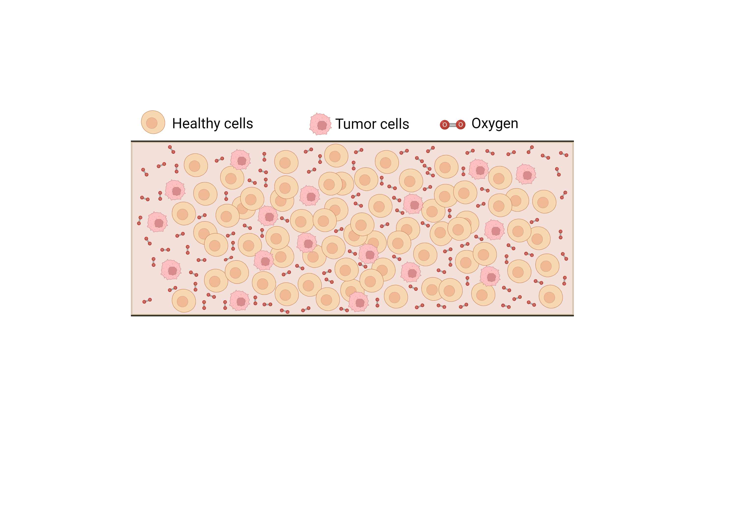
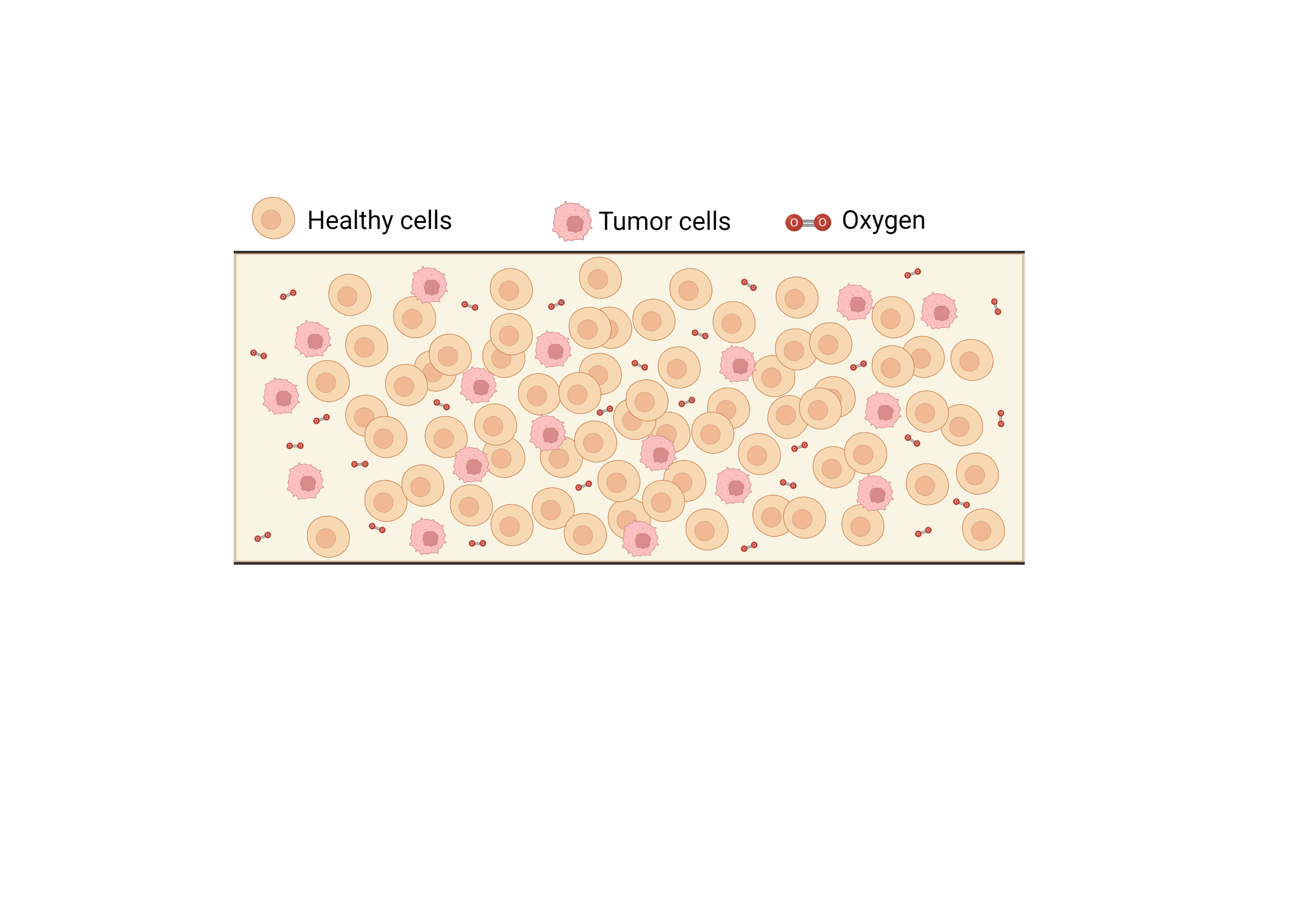
The presence of other cells in excess and high chemoattractant or oxygen levels.
With the assumptions and motivations as above in the derivation of Eq. (59) we now have
| (62a) | ||||
| (62b) | ||||
where the boundary conditions are again the ones given by Eqs. (48), except for the fact that the flux is given by as diffusion is neglected and the cell boundary condition at , with its associated boundary layer, is no longer considered as discussed in detail previously.
If we prescribe and , Eq. (62b) integrates to
| (63) |
We have therefore
and
for cell growth. Once more, this is a special case of with and , so the different functions needed in order to compute the solution are:
| (64a) | ||||
| (64b) | ||||
| (64c) | ||||
The expression of the cell profile may be computed using Eq. (13), which gives
| (65) |
where now
| (66) |
The evolution of the transition coordinate and the dimensionless cell profile for different times are shown in Fig. 10 for , , with , and a external stimulus given by and different shapes for .
While a fast oscillatory stimulus with plotted in Fig. 10 does not allow a ready approximation for cell density to the right of the transition region, we can consider the cases of or that are also considered in this Figure. In particular, we can use elementary but extensive manipulation to determine and approximate
to deduce that
in these cases. In particular, is of the form
for and
for .
For , we have with that
while, in contrast, for we note that
For both cases note that at fixed time the cell concentration to the right of the transition is essentially the exponential of a quadratic in , provided that is small enough.


Other cells and low chemoattractant or oxygen levels.
With analogous reasoning, Eqs. (49) now reduce to
| (67a) | ||||
| (67b) | ||||
The general solution to Eq. (67b) generates a chemotactic function that is neither linear in nor separable, with Eq. 6b equivalent to a Riccati differential equation in , for which general solutions are not known in terms of standard functions. Even though the general case is not tractable in terms of constructing solutions, two particular important configurations do allow progress, namely the gradient configuration ( and ) and the symmetric configuration (().
The gradient configuration is certainly the most interesting configuration. For that case, Eq. (67b) integrates to
| (68) |
whereby
Hence we have separability, with and . With
we in turn have
| (69a) | ||||
| (69b) | ||||
| (69c) | ||||
As with the previous cases the expression of the cell profile may be computed using Eq. (13), whereby
| (70) |
where , that is
| (71) |
and, with and constant, use of the change of variables reduces Eq. (70) to
The evolution of the transition coordinate and the dimensionless cell profile for different times are shown in Fig. 11 for , , , constant. Here, the cellular density to the right of transition further simplifies to
which entails for small time the spatial variation of the cellular density is that of a hyperbolic sine. Finally, note from the expression for and the fact for the transition zone to be within the domain, we have the bound so that the denominator in the above expression is positive and there is no singularity.
Even if less interesting from the experimental point of view, we can also obtain an expression for a symmetric configuration by considering half of the domain and applying Neumann boundary conditions for so Eq. (67b) is integrated to
| (72) |
Again we are under a separable case with and , so and , so the different functions needed in order to compute the solution are:
| (73a) | ||||
| (73b) | ||||
| (73c) | ||||


4 Discussion
There is an increasing use of in vitro investigations in the exploration of cellular motility, for instance with microdevice studies exploring tumour cell dynamics in response to oxygen gradients, as illustrated by GBM studies [51, 37, 40]. In turn this has motivated the main theme of this paper, namely modelling cell migration chemotaxis in heterogeneous environments, which applies for general chemoattractants, not just oxygen. In particular, the governing equations for cellular motility that have been considered are of the form
| (75) |
and supplemented by zero flux boundary conditions and suitable, typically constant, initial conditions. Furthermore, the general spatiotemporal heterogeneity in the chemotactic function and the growth function emerges from the chemoattractant gradients that the cells respond to, which may be manipulated extensively in microdevice experiments. However, the heterogeneity also entails that while cell migration dynamics towards high concentrations of chemoattractant is anticipated, the dynamics will not simply be that of a translationally invariant travelling wave and their associated analytical simplicity.
Hence, we have considered a framework capable of considering spatiotemporal chemotactic gradients and the resulting wavefront and cell density dynamics for cellular migrations in the presence of spatial and temporal heterogeneity. In particular, the fact cell spreading in the absence of chemotaxis is generally much slower than in its presence, the non-dimensional cellular diffusion coefficient is very small, so that typically , which we assume and exploit in this study. With this, we have that away from boundary layers near sources, which were located at the domain edge in the examples considered, and away from cell wavefronts with sharp transitions, an advection equation for the cellular density emerges with . Nonetheless, this advection equation is still complex, entailing that a constraint on constructing solutions for the cell density behaviour within the analytical framework presented here is that the chemotactic function must either be linear in or separable with respect to space and time. However, numerous cases are consistent with these constraints, as illustrated by the range of examples considered in Section 2.3, together with the examples that emerge from the consideration of cellular dynamics within microdevices in Section 3.
With these constraints, we have illustrated how the method of characteristics can be used to construct the cell density solutions away from boundary layers and transition regions, together with the use of boundary layer methods to construct a uniformly continuous approximate solution that accommodates the transition in the wavefront of the cells. In turn this provides an analytical characterisation of the movement of cellular wavefronts and the concentrations of cells within and either side of the wavefront. However we do not resolve boundary layers near oxygen sources, which has been the righthand boundary in the examples considered, for the presented framework given the limited insight the boundary layer will provide for the overall cell behaviour.
Even with the restriction of linearity or separability of the chemotactic functions , there is extensive freedom in the choices of and . Hence we first considered the predictions of the model for cell behaviour in exemplar test cases. In particular, we have explored and documented the behaviour of the cell density where the chemotactic function varies linearly in space and non-trivially in time, as well as quadratically in space and finally with exponential spatial behaviour. In addition to analytical investigations, we have also verified that the analytical solutions faithfully reproduce the behaviour of direct numerical solutions of the model, as may be observed extensively in Figures 3-7. Furthermore the exemplar solutions are subsequently used to study models reduced from a full coupling between the cellular density and chemoattractant concentration with a microdevice setting, as documented in Section 3. Once more the resulting dynamics are analytically investigated and documented, with rationally based analytical approximation for the location of the transition region and the cellular density presented.
Such analytical solutions are useful in numerous ways. For example, they provide oversight and insight for the system dynamics across parameter space. To illustrate, we consider the wavefront being driven by chemoattractant at the right hand boundary, so that . Then, with a measure of the strength of chemotaxis, differentiating from Eq. (64c) for the speed for the transition front gives
for the model of section 3.1.2, with high chemoattractant or oxygen levels. Hence, in this case, increasing the chemoattractant/oxygen uptake, as representing by increasing , always slows the propagation of a rightmoving wave. In contrast, for the model with low chemoattractant or oxygen levels of section 3.1.2 differentiating from Eq. (69c) we obtain
therefore revealing that increasing the chemoattractant/oxygen uptake always speeds up the propagation of rightmoving wave, illustrating the general deductions that may be made from the presented analytical solutions.
As well as providing analytical characterisation of the systems behaviour the analytical approximations provide a means to very rapidly compute cell behaviour. Thus the approximate analytical solutions can support computationally intensive studies. A simple example would be a global sensitivity analyses over all parameters. In particular, rapid evaluation would be most useful for parameter estimation using experimental, often noisy, data especially if Bayesian techniques are considered as this require extensive simulation to provide posterior distributions, rather than optimisation techniques which only generate point estimates for parameters. A directly analogous example is Bayesian model selection, whereby the comparison of experimental data and model prediction is used to distinguish different model structures when these are not known a priori, such as different functional forms of or representing different prospective growth and chemotactic responses for a given the tumour cell line in question. In particular both optimisation techniques and the Bayesian techniques are iterative, so that the use of a rational but rapid evaluation of an approximation to an optimum in optimisation studies or a posterior for Bayesian techniques can in turn be used to restart the procedure with the full numerical model to further refine the results [52].
In summary, we have developed a framework for the construction of analytical approximations for front behaviours and densities for cells undergoing chemotaxis in heterogeneous environments, as characterised by the chemotactic and growth functions and respectively. The resulting cellular waves of migration are not simple travelling waves due to the heterogeneity induced by the chemoattractant profiles. Nonetheless, numerous features of the wavefronts have been extracted via rational approximation, such as the location and speed of the propagating wave, together with the cellular density profile. These have been explored and validated for exemplars scenarios as well as investigated for models fundamentally motivated by experimental microdevices for observing cellular motility under a very wide range of conditions, even if complete generality is not feasible for progress using constructive methods. Thus, the solutions presented here not only provide insight into the behaviour of cellular motility under the influence of spatiotemporal chemotactic heterogeneity, but also highlight general behaviours and important mechanisms and parameters, as well as providing a means of rapid evaluation in demanding computational studies, such as Bayesian parameter estimation and model selection.
Aknowledgements
The authors gratefully acknowledge the financial support from the Spanish Ministry of Science and Innovation (MICINN), the State Research Agency (AEI), and FEDER, UE through the projects PID2019-106099RB-C44/AEI and PID2021-126051OB-C41, the Government of Aragon (DGA) and the “Centro de Investigación Biomedical en Red en Bioingeniería, Biomateriales y Nanomedicina (CIBER-BBN)”, financed by the Instituto de Salud Carlos III with assistance from the European Regional Development Fund (FEDER).
References
- [1] Christopher S Chen, Milan Mrksich, Sui Huang, George M Whitesides, and Donald E Ingber. Geometric control of cell life and death. Science, 276(5317):1425–1428, 1997.
- [2] ASG Curtis and GM Seehar. The control of cell division by tension or diffusion. Nature, 274(5666):52, 1978.
- [3] Ulrich S Schwarz and Ilka B Bischofs. Physical determinants of cell organization in soft media. Medical Engineering & Physics, 27(9):763–772, 2005.
- [4] Stephen B Carter. Haptotaxis and the mechanism of cell motility. Nature, 213(5073):256, 1967.
- [5] Chun-Min Lo, Hong-Bei Wang, Micah Dembo, and Yu-li Wang. Cell movement is guided by the rigidity of the substrate. Biophysical Journal, 79(1):144–152, 2000.
- [6] Dennis Bray. Cell movements: from molecules to motility. Garland Science, 2000.
- [7] Seyed Jamaleddin Mousavi, Mohamed Hamdy Doweidar, and Manuel Doblaré. 3d computational modelling of cell migration: a mechano-chemo-thermo-electrotaxis approach. Journal of Theoretical Biology, 329:64–73, 2013.
- [8] Vinay Kumar, AK Abbas, and JC Aster. Cell injury, cell death, and adaptations. Robbins Basic Pathology, 8:1–30, 2013.
- [9] Seyed Jamaleddin Mousavi, Manuel Doblaré, and Mohamed Hamdy Doweidar. Computational modelling of multi-cell migration in a multi-signalling substrate. Physical Biology, 11(2):026002, 2014.
- [10] Sui Huang and Donald E Ingber. Cell tension, matrix mechanics, and cancer development. Cancer Cell, 8(3):175–176, 2005.
- [11] Douglas Hanahan and Robert A Weinberg. Hallmarks of cancer: the next generation. Cell, 144(5):646–674, 2011.
- [12] Anika Nagelkerke, Johan Bussink, Alan E Rowan, and Paul N Span. The mechanical microenvironment in cancer: How physics affects tumours. In Seminars in cancer biology, volume 35, pages 62–70. Elsevier, 2015.
- [13] Daniela F Quail and Johanna A Joyce. Microenvironmental regulation of tumor progression and metastasis. Nature Medicine, 19(11):1423–1437, 2013.
- [14] SJ Mousavi, MH Doweidar, and M Doblaré. Cell migration and cell-cell interaction in the presence of mechano-chemo-thermotaxis. Mol Cell Biomech, 10(1):1–25, 2013.
- [15] Jack W Scannell, Alex Blanckley, Helen Boldon, and Brian Warrington. Diagnosing the decline in pharmaceutical r&d efficiency. Nature reviews Drug Discovery, 11(3):191–200, 2012.
- [16] Garry P Nolan. What’s wrong with drug screening today. Nature Chemical Biology, 3(4):187–191, 2007.
- [17] Rasheena Edmondson, Jessica Jenkins Broglie, Audrey F Adcock, and Liju Yang. Three-dimensional cell culture systems and their applications in drug discovery and cell-based biosensors. Assay and Drug Development Technologies, 12(4):207–218, 2014.
- [18] Chengyang Wang, Zhenyu Tang, Yu Zhao, Rui Yao, Lingsong Li, and Wei Sun. Three-dimensional in vitro cancer models: a short review. Biofabrication, 6(2):022001, 2014.
- [19] Eric K Sackmann, Anna L Fulton, and David J Beebe. The present and future role of microfluidics in biomedical research. Nature, 507(7491):181–189, 2014.
- [20] Sangeeta N Bhatia and Donald E Ingber. Microfluidic organs-on-chips. Nature Biotechnology, 32(8):760, 2014.
- [21] Simone Bersini, Jessie S Jeon, Gabriele Dubini, Chiara Arrigoni, Seok Chung, Joseph L Charest, Matteo Moretti, and Roger D Kamm. A microfluidic 3d in vitro model for specificity of breast cancer metastasis to bone. Biomaterials, 35(8):2454–2461, 2014.
- [22] Alexandra Boussommier-Calleja, Ran Li, Michelle B Chen, Siew Cheng Wong, and Roger D Kamm. Microfluidics: a new tool for modeling cancer–immune interactions. Trends in Cancer, 2(1):6–19, 2016.
- [23] Jessie S Jeon, Simone Bersini, Mara Gilardi, Gabriele Dubini, Joseph L Charest, Matteo Moretti, and Roger D Kamm. Human 3d vascularized organotypic microfluidic assays to study breast cancer cell extravasation. Proceedings of the National Academy of Sciences, 112(1):214–219, 2015.
- [24] Ioannis K Zervantonakis, Shannon K Hughes-Alford, Joseph L Charest, John S Condeelis, Frank B Gertler, and Roger D Kamm. Three-dimensional microfluidic model for tumor cell intravasation and endothelial barrier function. Proceedings of the National Academy of Sciences, 109(34):13515–13520, 2012.
- [25] Danli Wu and Patricia Yotnda. Induction and testing of hypoxia in cell culture. JoVE (Journal of Visualized Experiments), (54):e2899, 2011.
- [26] Helen M Byrne. Dissecting cancer through mathematics: from the cell to the animal model. Nature Reviews Cancer, 10(3):221–230, 2010.
- [27] Philipp M Altrock, Lin L Liu, and Franziska Michor. The mathematics of cancer: integrating quantitative models. Nature Reviews Cancer, 15(12):730–745, 2015.
- [28] Hiroaki Kitano. Computational systems biology. Nature, 420(6912):206, 2002.
- [29] Elaine L Bearer, John S Lowengrub, Hermann B Frieboes, Yao-Li Chuang, Fang Jin, Steven M Wise, Mauro Ferrari, David B Agus, and Vittorio Cristini. Multiparameter computational modeling of tumor invasion. Cancer Research, 69(10):4493–4501, 2009.
- [30] R Eils and AE Kriete. Computational systems biology: from molecular mechanisms to disease. Academic, New York, NY, 2013.
- [31] HM Byrne, T Alarcon, MR Owen, SD Webb, and PK Maini. Modelling aspects of cancer dynamics: a review. Philosophical Transactions of the Royal Society A: Mathematical, Physical and Engineering Sciences, 364(1843):1563–1578, 2006.
- [32] Moriah E Katt, Amanda L Placone, Andrew D Wong, Zinnia S Xu, and Peter C Searson. In vitro tumor models: advantages, disadvantages, variables, and selecting the right platform. Frontiers in Bioengineering and Biotechnology, 4:12, 2016.
- [33] Daniel J Brat. Glioblastoma: biology, genetics, and behavior. American Society of Clinical Oncology Educational Book, 32(1):102–107, 2012.
- [34] Haralampos Hatzikirou, Andreas Deutsch, Carlo Schaller, Matthias Simon, and Kristin Swanson. Mathematical modelling of glioblastoma tumour development: a review. Mathematical Models and Methods in Applied Sciences, 15(11):1779–1794, 2005.
- [35] Yangjin Kim, Hyejin Jeon, and Hans Othmer. The role of the tumor microenvironment in glioblastoma: A mathematical model. IEEE Transactions on Biomedical Engineering, 64(3):519–527, 2016.
- [36] Haralampos Hatzikirou, David Basanta, Matthias Simon, K Schaller, and Andreas Deutsch. ‘go or grow’: the key to the emergence of invasion in tumour progression? Mathematical Medicine and Biology: a journal of the IMA, 29(1):49–65, 2012.
- [37] Jose M Ayuso, Rosa Monge, Alicia Martínez-González, María Virumbrales-Muñoz, Guillermo A Llamazares, Javier Berganzo, Aurelio Hernández-Laín, Jorge Santolaria, Manuel Doblaré, Christopher Hubert, et al. Glioblastoma on a microfluidic chip: generating pseudopalisades and enhancing aggressiveness through blood vessel obstruction events. Neuro-Oncology, 19(4):503–513, 2017.
- [38] Alicia Martínez-González, Gabriel F Calvo, Luis A Pérez Romasanta, and Víctor M Pérez-García. Hypoxic cell waves around necrotic cores in glioblastoma: a biomathematical model and its therapeutic implications. Bulletin of Mathematical Biology, 74(12):2875–2896, 2012.
- [39] Hermann B Frieboes, Xiaoming Zheng, Chung-Ho Sun, Bruce Tromberg, Robert Gatenby, and Vittorio Cristini. An integrated computational/experimental model of tumor invasion. Cancer Research, 66(3):1597–1604, 2006.
- [40] Jacobo Ayensa-Jiménez, Marina Pérez-Aliacar, Teodora Randelovic, Sara Oliván, Luis Fernández, José Antonio Sanz-Herrera, Ignacio Ochoa, Mohamed H Doweidar, and Manuel Doblaré. Mathematical formulation and parametric analysis of in vitro cell models in microfluidic devices: application to different stages of glioblastoma evolution. Scientific Reports, 10(1):1–21, 2020.
- [41] Marina Pérez-Aliacar, Mohamed H Doweidar, Manuel Doblaré, and Jacobo Ayensa-Jiménez. Predicting cell behaviour parameters from glioblastoma on a chip images. a deep learning approach. Computers in Biology and Medicine, page 104547, 2021.
- [42] Víctor M Pérez-García, Gabriel F Calvo, Juan Belmonte-Beitia, David Diego, and Luis Pérez-Romasanta. Bright solitary waves in malignant gliomas. Physical Review E, 84(2):021921, 2011.
- [43] Philip Gerlee and Sven Nelander. Travelling wave analysis of a mathematical model of glioblastoma growth. Mathematical biosciences, 276:75–81, 2016.
- [44] Tracy L Stepien, Erica M Rutter, and Yang Kuang. Traveling waves of a go-or-grow model of glioma growth. SIAM Journal on Applied Mathematics, 78(3):1778–1801, 2018.
- [45] Evelyn F Keller and Lee A Segel. Traveling bands of chemotactic bacteria: a theoretical analysis. Journal of theoretical biology, 30(2):235–248, 1971.
- [46] Gurusamy Arumugam and Jagmohan Tyagi. Keller-segel chemotaxis models: a review. Acta Applicandae Mathematicae, 171(1):1–82, 2021.
- [47] Chuan Xue, Hyung Ju Hwang, Kevin J Painter, and Radek Erban. Travelling waves in hyperbolic chemotaxis equations. Bulletin of Mathematical Biology, 73(8):1695–1733, 2011.
- [48] Yoojin Shin, Sewoon Han, Jessie S Jeon, Kyoko Yamamoto, Ioannis K Zervantonakis, Ryo Sudo, Roger D Kamm, and Seok Chung. Microfluidic assay for simultaneous culture of multiple cell types on surfaces or within hydrogels. Nature Protocols, 7(7):1247–1259, 2012.
- [49] Athel Cornish-Bowden. The origins of enzyme kinetics. FEBS Letters, 587(17):2725–2730, 2013.
- [50] Archibald Vivian Hill. The possible effects of the aggregation of the molecules of haemoglobin on its dissociation curves. J. Physiol., 40:4–7, 1910.
- [51] Jose M Ayuso, María Virumbrales-Muñoz, Alodia Lacueva, Pilar M Lanuza, Elisa Checa-Chavarria, Pablo Botella, Eduardo Fernández, Manuel Doblare, Simon J Allison, Roger M Phillips, et al. Development and characterization of a microfluidic model of the tumour microenvironment. Scientific Reports, 6(1):1–16, 2016.
- [52] Liam V Brown, Jonathan Wagg, Rachel Darley, Andy van Hateren, Tim Elliott, Eamonn A Gaffney, and Mark C Coles. De-risking clinical trial failure through mechanistic simulation. Immunotherapy Advances, 2(1):ltac017, 2022.
- [53] Frank Olver. Asymptotics and special functions. CRC Press, 1997.
Appendix A Oscillatory solutions for homogeneous growth
We consider homogeneous growth, so that is a constant independent of and , together with a temporally oscillating chemotactic response governed by , so that Eq. (24) reduces to
| (76) |
Hence the cell concentration to the right of the transition region, but away from the boundary layer at , is spatially constant with a temporal oscillation, which we consider below for four distinct parameter regimes.
A.1 Slow variations of the gradients,
Let and, without loss of generality, we consider the decomposition . Then, Eq. (76) becomes
| (77) |
Further, let , so we have
| (78) |
Since , we can approximate the solution of Eq. (78) by
| (79) |
As we have a slow modulation of the frequency/decay rate, we use the Wentzel-Kramers-Brillouin (WKB) method [53]. In terms of , Eq. (80) becomes
| (82) |
The WKB approximation is expressed here as
| (83) |
Therefore, , so that
| (85) |
The corresponding equation is
| (86) |
and solving it for gives
| (87) |
The corresponding equation is
| (88) |
so, as , we obtain (constant).
Consequently, Eq. (83) becomes
| (89) |
for constant. Using that and the initial value , we obtain the approximation
| (90) |
Finally, as , we have
| (91) |
A.2 Fast variations of the gradients,
We solve now the problem using the method of multiple scales. Let us assume that , where and , so that
| (92) |
If , Eq. (76) becomes
| (93) |
If we use an asymptotic expansion of , we obtain:
| (94) |
Solving the equation obtained collecting the terms, we find is a function of only, that is
| (95) |
with the initial condition
Now, for the equation obtained collecting the terms, we have
| (96) |
As is a periodic correction, integrating Eq. (96) over we obtain
| (97) |
and thus, solving for , we have
| (98) |
Hence, the leading order approximation is
| (99) |
Now, for the equation we have:
| (100) |
Since ,
| (101) |
and therefore the first order correction is, , that is:
| (102) |
A.3 Dominant chemotaxis,
We solve now the problem using the standard asymptotic expansion method. We set . Then, Eq. (76) reduces to
| (103) |
The leading order solution is obtained immediately as it is the solution to the homogeneous linear differential equation:
| (104) |
Thus the leading order approximation is
| (105) |
though the next order correction generates a cumbersome expression and thus is not presented.
A.4 Dominant cell proliferation,
Again, we solve the problem using the standard asymptotic expansion method. Now, we set . Then, Eq. (76) gives
| (106) |
The leading order solution is obtained immediately as the solution to the inhomogeneous linear differential equation
| (107) |
and hence is given by
| (108) |
For the first correction, an asymptotic expansion of of the form reveals that
| (109) |
The solution to this ODE with initial condition is given by
| (110) |
where we have defined . Hence up to the first order correction we have
| (111) |
Appendix B Simplification of the transport equation for chemotaxis
With denoting the concentration of the chemoattractant, and with we have in section 3.1 an equation of the form
since has been imposed on (49b), while in section 3.1.2 we have equations of one of the two forms
via Equations (58), (60) respectively. These are accompanied by boundary conditions of the form
and initial conditions are required to close the system. For simplicity, we assume the boundary conditions and initial conditions are consistent at .
To further proceed we firstly assume , so that can be treated as unit order of magnitude in asymptotic methods based on , and we also assume that have derivatives that are unit order of magnitude, or less. With these weak assumptions, our objective is show that the time derivative can be neglected at leading order, justifying the use of Eqs. (50b), (59), (61) in the main text and also justifying the neglect of the consideration of initial conditions in the main text on the grounds this only governs fast initial transients.
Below we work with the PDE
| (112) |
with so that gives one the above equations while , gives another with the final possibility corresponding to , allowing the three cases to be considered simultaneously.
We have an outer timescale of and an inner timescale of . In the outer region, , for the leading order outer solution one indeed has
without consideration of the initial condition. Hence the solutions presented in the main text, for instance Eqs. (51), (63),(68),(72), are the same as the leading order outer solutions. With the leading order inner solution we have
and the leading order boundary conditions
on noting and where corrections are dropped in the final term for both boundary conditions. Recalling and using the decomposition
without loss of generality, we have
With the Fourier decomposition of and its initial condition
we have
so that
Thus the leading order composite solution is given by
| (113) | |||||
Thus, as implemented in the main text, working solely with the outer solution and neglecting the initial conditions is a rational asymptotic approximation at leading order with respect to , once initial transients have decayed, that is for times satisfying . As the initial transients, and very short times, are not of interest for determining the behaviour of the invasive front of cells for the majority of its propagation we thus work only with the outer equations and solution in the main text.