Parametrized quasi-normal mode framework for non-Schwarzschild metrics
Abstract
In this work we comment in more detail on what happens to the parametrized framework first presented by Cardoso et al. when there are departures from the Schwarzschild background metric, as well as possible deviations in the “dynamics”. We treat possible deviations in the background metric with additional coefficients with respect to the original works. The advantages of this reformulation are clear when applied to a parameter estimation problem, since the coefficients are always real, and many of them do not depend on the overtone number and angular momentum of the frequency, thus eventually reducing the total amount of parameters to be inferred.
I Introduction
Ongoing and future efforts of gravitational wave detectors provide unprecedented access to test general relativity (GR) in the strong field regime Abbott et al. 2016; Abbott et al. 2019; Abbott et al. 2021a; Abbott et al. 2021b. Among the several exciting possibilities, one is to perform black hole spectroscopy in order to verify the validity of the requirements of the no-hair theorem and also general relativity itself Kerr 1963; Carter 1971; Robinson 1975. Our current understanding of binary black hole mergers predicts that the final stage of such events should be described by a superposition of linear perturbations of the background, the so-called quasi-normal modes Regge and Wheeler 1957; Zerilli 1970; Teukolsky 1973, see also Refs. Kokkotas and Schmidt 1999; Nollert 1999; Berti et al. 2009; Konoplya and Zhidenko 2011 for reviews.
The spectrum of quasi-normal modes is sensitive to the background perturbed metric, but also to the dynamical behaviour of the theory in which the perturbations are excited. The purpose of this work is to provide a framework which allows one to study quasi-normal modes in spherical symmetry for metrics which are different from the Schwarzschild metric when the modifications are small. Our framework follows a prescription similar to the one presented by Cardoso et al. Cardoso et al. 2019 and McManus et al. McManus et al. 2019. In these works, a modified (system) of wave equations has been introduced and the corresponding quasi-normal mode spectrum has been computed up to quadratic order for a set of small deviation parameters. We explicitly show how possible deviations in the background metric could affect the quasi-normal frequencies, in a different fashion compared to Cardoso et al. 2019; McManus et al. 2019. While the general idea is similar, our approach allows for a better description of non-Schwarzschild backgrounds, purely real deviation parameters in the framework, as well as a differentiation between the parameters that depend on the angular momentum of the frequencies and those which do not.
II Theoretical Framework
Let us start by qualitatively reviewing how gravitational perturbations in gravity theories can be studied. In general, one assumes a linear perturbation of the metric as
| (1) |
for which the background metric and the perturbation metric satisfy the 0th order and 1st order equations of motion, respectively. They are obtained from the linear expansion of the full system of equations
| (2) |
where are the equations of motion of a given gravity theory. Let us assume that the background metric is given by some non-GR metric. We remark that we do not know a priori which equations of motion this metric is satisfying. However, as long as it is perturbatively close, with respect to some parameter , to the Schwarzschild/Kerr metric, it must satisfy Einstein’s equations of GR up to some error linear in ,
| (3) |
The presence of the term can be interpreted as the fact that the equations of motion of a new theory whose static solution is approximated by the metric must have different dynamics, not captured with the GR equations by a linear factor.
We can conjecture that the first order equations share the same property. For GR, one would have
| (4) |
but when is substituted by , the equations become
| (5) |
One must bear in mind that this notation generically includes the 0th and 1st order metric as well as their derivatives.
Let us now take into account a spherically symmetric background metric defined as follows
| (6) |
with , being the location of the event horizon. Then, we can expand the functions and with a set of real coefficients in a post-Newtonian fashion Barausse et al. 2014
| (7) | ||||
| (8) |
We make the series terminate at some finite number starting from to ensure asymptotic flatness.
From the prescription suggested by passing from Eq. (4) to Eq. (5) one could guess the following form for the master perturbation equation
| (9) |
where one has enough generality to define the perturbation variable to choose such that the tortoise coordinate arising from this equation is . Finally, we expect small deviations from GR in the other parameters as well: , . Note that in this definition we made explicit that radial functions modifying the potential depend on the angular momentum of the quasi-normal frequencies.
In the following we try to provide a heuristic explanation for why we expect this form for the master equation. The first step is to write down the master equation for a perturbation in GR
| (10) |
where is the “natural” tortoise function for the Schwarzschild solution, and
| (11) |
where , denotes scalar perturbations, for axial perturbations and
| (12) |
for polar perturbations. We intentionally wrote the eikonal term to make its correspondence with geodesic motion evident.
If we assume that the background metric is the metric of Eq. (6), we can substitute all the terms with everywhere in equation (10). For example, one should transform into . Moreover, to take into account that the theory can be different, one should add a correction to the tortoise coordinate and one to the potential. These two corrections take into account the fact that the derivation of the perturbation equation might be done in a theory which is not GR [cf. Eq. (5)]. The resulting equation is
| (13) |
One can always re-define the perturbation function and re-scale the equation to remove the term from the derivative term. This would ensure that the second order derivative is acted upon the tortoise coordinate of the metric. However, by doing so, one would introduce some terms multiplying the frequency, obtaining Eq. (9). The term multiplying the frequency can be mapped into the modification of the tortoise coordinate , and we expand it as
| (14) |
It is worth noting that this term appears because the background metric (and thus the tortoise coordinate) is different from the Schwarzschild metric.
On the potential side, from the construction, we can split the contribution to the potential coming from the metric and from the “dynamics”. We have that
| (15) |
where we made the following identifications:
| (16) | ||||
| (17) |
This last term, linear in , expresses in a basis our ignorance on the correct equations of motion for the dynamics of the theories under scrutiny.
Collectively we label all the real coefficients, from metric and from dynamics as
| (18) |
where we identified from the definition of . In the rest of the paper we will refer to this set of parameters as mixed parametrization or metric-potential parametrization to distinguish it from the potential-only parametrization introduced in Cardoso et al. 2019. A quadratic expansion of in the parameters is simply given by
| (19) |
We can infer the coefficients and from the coefficients and obtained in Cardoso et al. 2019; McManus et al. 201911 1 See also Kimura 2020; Völkel et al. 2022a for alternative ways to compute these coefficients by comparing the respective master equations. In order to do so, we must manipulate Eq. (9). By performing the change of variables , the master equation takes the form
| (20) | |||
| (21) |
with and . In addition, the last term of (21) can be put in the form with the following manipulation:
| (22) |
In this way, we can define a first order expansion of the potential in as
| (23) |
The coefficients can be obtained up to second-order by combinations of the coefficients . For generic index and tensor axial perturbation, we have that linear contributions are
| (24) |
while we do not display the quadratic ones since the expression is lengthy and uninformative. The formula for scalar perturbations has an analogous form, while for the tensor polar case, one should first decompose the term (12) such that it yields terms. We suggest that the best-motivated way to proceed is to perform an eikonal expansion of the term (i.e., around ) and include eikonal terms until the deviation in the coefficients is smaller than the numerical error of the coefficients themselves.
The manipulation shown with the previous calculations results in equation (20) being the same form as that in Ref. Cardoso et al. 2019. Now, one can apply the quadratic expansion of the quasi-normal frequencies from Refs. Cardoso et al. 2019; McManus et al. 2019 to Eq. (20), yielding
| (25) |
Due to the relation between the coefficients and , we can always do the mapping
| (26) | ||||
| (27) |
It is worth noting that since all the coefficients are real, any term that would make the coefficients complex comes from the fact that the background metric is not Schwarzschild. Indeed, we note that the coefficients denote the deviation of the “natural” tortoise coordinate of the master equation from the tortoise coordinate of the metric, nonetheless defined by the coefficients .22 2 An additional frequency-dependent contribution not shown here could come from a non-spherically symmetric background metric, that reduces to Schwarzschild in the zero coupling limit (e.g., the slow-rotation expansion Pani 2013).
The advantage of this formulation over the potential-only parametrization is evident when reconstructing the modified potential after the detection of more than one quasi-normal mode Völkel and Barausse 2020; Völkel et al. 2022a; Völkel et al. 2022b. In fact, even at first it seems that the metric-potential formalism has more parameters than the potential-only one, one must be aware that the coefficients of the latter are complex (because they can depend on the frequency) and they are different for each mode measured, as they are sensitive to and . This means twice as many coefficients for each mode measured. On the other hand, the mixed formalism has coefficients which change with the angular momentum of the mode, and coefficients , and . None of them depends on the overtone number. By simple counting, one can find that the total number of coefficients for the observation of different angular momentum modes and additional (i.e., on top of the fundamental one) overtones for the potential-only case is , while for the metric-potential case, one has .
Formally the mapping to the metric can also be extended to cover the more general scenario of a coupled system of equations, as studied in Ref. McManus et al. 2019, if one makes similar assumptions about how the fields are coupled to each other. Those key assumptions are that the additional coupling functions can be expressed in a similar expansion scheme as the potential in eq. (23) and that the additional fields couple linearly via the coupling functions. Such a structure of the coupled case has been explored in Ref. McManus et al. 2019 for dynamical Chern-Simons, Horndeski gravity and an effective field theory approach.
III Applications
III.1 Reissner-Nordström metric
As first non-trivial application of the framework we consider the Reissner-Nordström (RN) metric Reissner 1916; Weyl 1917; Nordström 1918; Jeffery 1921. With the current notation it is given by the metric Eq. (6), with
| (28) |
where can be related to the mass and a (small) electric charge through
| (29) |
and the location of the horizon is given by
| (30) |
The perturbation equation in the odd-parity sector is close to the Regge-Wheeler equation Berti et al. 2009. From its expression, one can either infer the axial deviation parameters for potential-only formalism (cfr. Ref. Cardoso et al. 2019) or the parameters for the mixed framework
| (31) | ||||
| (32) |
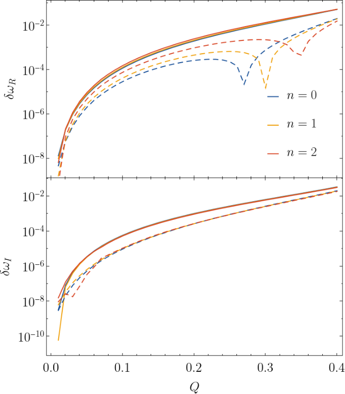
In Fig. 1 we compare the application of the original parametrized framework with the new metric dependent one for the RN , quasi-normal modes. In the two panels we show the relative error between the parametrized quasi-normal modes (potential-only parametrization is represented by solid lines while potential-metric parametrization by dashed lines) and the numerically computed one . We check that from the scaling of the relative error, the deviation of RN QNMs from Schwarzschild QNMs is much larger than the error introduced by the parametrization, for the parameters considered. One can clearly see that the mixed parametrization gives an even more accurate prediction of the frequencies for each case considered. We also checked different angular momentum which gives analogous features.
III.2 Einstein-dilaton-Gauss-Bonnet gravity
Einstein-dilaton-Gauss-Bonnet (EdGB) gravity is a well-studied alternative theory of gravity, where a dynamical scalar field is coupled to the Gauss-Bonnet invariant through a coupling . Our notation for the action of the theory and the equations of motion is consistent with that of Ref. Bryant et al. 2021. Further information about the theory can be found in the latter, as well as in Ref. Julié and Berti 2019 and references therein. In the small-coupling limit, unless the coupling function does not have a linear term in the scalar field, all BHs in the theory develop a scalar profile around them, and the background metric and the perturbation equations are of the form we analysed here. The QNM spectrum of these solutions was computed in Ref. Blázquez-Salcedo et al. 2016 without the small coupling expansion. The master equation for axial perturbation can be recast in the form of Eq. (9) retaining up to terms, where we introduced the dimensionless coupling . The relevant functions are (according to the notation of Bryant et al. 2021)
| (33) | ||||
| (34) | ||||
| (35) |
| (36) |
As shown in section II, one can transform the equation such that it is in the form suitable to express the modifications from GR as coefficients of the potential formalism. Hence, in Fig. 2, we compare the fundamental modes obtained with the two different formalisms against the fits of the numerical quasi-normal mode frequencies computed in Blázquez-Salcedo et al. 2016. In this case, the metric-potential parametrization under-performs the potential-only one in most cases, even though the error with respect to the numerical fits are still comparable.

IV Conclusions
In this work we have introduced a framework to compute quasi-normal modes from non-GR metrics where modifications are small. Our ansatz is very similar and can be mapped to the one proposed by Cardoso et al. Cardoso et al. 2019. This allows for a quick computation of QNMs of a given metric. We have found comparable precision among the two methods in approximating the numerically computed frequencies both for RN and EdGB axial perturbations. We showed how to perform the mapping between the two formalisms for scalar and tensor axial perturbations only, but we also provided an explanation on how to do it for the tensor polar case.
The main advantage of the mixed method is evident when one has in mind the so-called inverse problem, which refers to the reconstruction of the perturbation equation in a theory-agnostic approach Völkel and Barausse 2020; Völkel et al. 2022a; Völkel et al. 2022b. The essential condition for the inverse problem is the detection of more angular modes/overtones simultaneously, even if the capability of doing so with current observations resulted in an ongoing discussion in the literature Isi et al. 2019; Capano et al. 2021; Cotesta et al. 2022; Finch and Moore 2022; Isi and Farr 2022; Capano et al. 2022. The advantage in the inverse problem comes from a reduction of the number of parameters, all real, and only with the depending on the angular momentum of the perturbation. This is not the case for the potential-only parametrization, for which all coefficients are, in principle, complex and depend on angular momentum and overtone number as well. Moreover, it can give insight into discerning whether a modification comes from the background or from the dynamics.
The possibility to explicitly separate the two contributions could also be useful when complementary constraints on the metric are provided, but not on the dynamics. Such a case may be possible with activities of the Event Horizon Telescope Collaboration Akiyama et al. 2019a; Akiyama et al. 2019b; Akiyama et al. 2022a, which can, in principle, be used to study possible deviations from the Schwarzschild/Kerr metric of supermassive black holes, see e.g. Refs. Psaltis et al. 2020; Völkel et al. 2021; Kocherlakota et al. 2021; Nampalliwar and K 2021; Lara et al. 2021; Kocherlakota and Rezzolla 2022; Ayzenberg 2022; Akiyama et al. 2022b for some recent works. Other complementary constraints can also be obtained using x-ray spectroscopy; see, e.g., Refs. Bambi et al. 2017; Tripathi et al. 2019; Cardenas-Avendano et al. 2020. Although it seems unlikely that observations of the same objects can be done using gravitational waves and one of these techniques in the foreseeable future, one can still combine constraints on individual metrics under certain assumptions, e.g., assuming that the way the metric is modified is similar for all sources.
Acknowledgements.
We thank Enrico Barausse, Andrea Maselli and Masashi Kimura for providing feedback on the final version of the manuscript. We acknowledge financial support provided under the European Union’s H2020 ERC Consolidator Grant “GRavity from Astrophysical to Microscopic Scales” grant agreement no. GRAMS-815673. S.V. acknowledges funding from the Deutsche Forschungsgemeinschaft (DFG) - project number: 386119226.References
- Abbott et al. (2016) B. P. Abbott et al. (LIGO Scientific, Virgo), Tests of general relativity with GW150914, Phys. Rev. Lett. 116, 221101 (2016), [Erratum: Phys.Rev.Lett. 121, 129902 (2018)], arXiv:1602.03841 [gr-qc] .
- Abbott et al. (2019) B. P. Abbott et al. (LIGO Scientific, Virgo), GWTC-1: A Gravitational-Wave Transient Catalog of Compact Binary Mergers Observed by LIGO and Virgo during the First and Second Observing Runs, Phys. Rev. X 9, 031040 (2019), arXiv:1811.12907 [astro-ph.HE] .
- Abbott et al. (2021a) R. Abbott et al. (LIGO Scientific, Virgo), GWTC-2: Compact Binary Coalescences Observed by LIGO and Virgo During the First Half of the Third Observing Run, Phys. Rev. X 11, 021053 (2021a), arXiv:2010.14527 [gr-qc] .
- Abbott et al. (2021b) R. Abbott et al. (LIGO Scientific, VIRGO, KAGRA), GWTC-3: Compact Binary Coalescences Observed by LIGO and Virgo During the Second Part of the Third Observing Run, (2021b), arXiv:2111.03606 [gr-qc] .
- Kerr (1963) R. P. Kerr, Gravitational field of a spinning mass as an example of algebraically special metrics, Phys. Rev. Lett. 11, 237 (1963).
- Carter (1971) B. Carter, Axisymmetric black hole has only two degrees of freedom, Phys. Rev. Lett. 26, 331 (1971).
- Robinson (1975) D. C. Robinson, Uniqueness of the kerr black hole, Phys. Rev. Lett. 34, 905 (1975).
- Regge and Wheeler (1957) T. Regge and J. A. Wheeler, Stability of a Schwarzschild singularity, Phys. Rev. 108, 1063 (1957).
- Zerilli (1970) F. J. Zerilli, Effective potential for even parity Regge-Wheeler gravitational perturbation equations, Phys. Rev. Lett. 24, 737 (1970).
- Teukolsky (1973) S. A. Teukolsky, Perturbations of a rotating black hole. 1. Fundamental equations for gravitational electromagnetic and neutrino field perturbations, Astrophys. J. 185, 635 (1973).
- Kokkotas and Schmidt (1999) K. D. Kokkotas and B. G. Schmidt, Quasinormal modes of stars and black holes, Living Rev. Rel. 2, 2 (1999), arXiv:gr-qc/9909058 .
- Nollert (1999) H. P. Nollert, Topical review: Quasinormal modes: the characteristic ‘sound’ of black holes and neutron stars, Class. Quant. Grav. 16, R159 (1999).
- Berti et al. (2009) E. Berti, V. Cardoso, and A. O. Starinets, Quasinormal modes of black holes and black branes, Class. Quant. Grav. 26, 163001 (2009), arXiv:0905.2975 [gr-qc] .
- Konoplya and Zhidenko (2011) R. A. Konoplya and A. Zhidenko, Quasinormal modes of black holes: From astrophysics to string theory, Rev. Mod. Phys. 83, 793 (2011), arXiv:1102.4014 [gr-qc] .
- Cardoso et al. (2019) V. Cardoso, M. Kimura, A. Maselli, E. Berti, C. F. B. Macedo, and R. McManus, Parametrized black hole quasinormal ringdown: Decoupled equations for nonrotating black holes, Phys. Rev. D 99, 104077 (2019), arXiv:1901.01265 [gr-qc] .
- McManus et al. (2019) R. McManus, E. Berti, C. F. B. Macedo, M. Kimura, A. Maselli, and V. Cardoso, Parametrized black hole quasinormal ringdown. II. Coupled equations and quadratic corrections for nonrotating black holes, Phys. Rev. D 100, 044061 (2019), arXiv:1906.05155 [gr-qc] .
- Barausse et al. (2014) E. Barausse, V. Cardoso, and P. Pani, Can environmental effects spoil precision gravitational-wave astrophysics?, Phys. Rev. D 89, 104059 (2014), arXiv:1404.7149 [gr-qc] .
- Kimura (2020) M. Kimura, Note on the parametrized black hole quasinormal ringdown formalism, Phys. Rev. D 101, 064031 (2020), arXiv:2001.09613 [gr-qc] .
- Völkel et al. (2022a) S. H. Völkel, N. Franchini, and E. Barausse, Theory-agnostic reconstruction of potential and couplings from quasinormal modes, Phys. Rev. D 105, 084046 (2022a), arXiv:2202.08655 [gr-qc] .
- Pani (2013) P. Pani, Advanced Methods in Black-Hole Perturbation Theory, Int. J. Mod. Phys. A 28, 1340018 (2013), arXiv:1305.6759 [gr-qc] .
- Völkel and Barausse (2020) S. H. Völkel and E. Barausse, Bayesian Metric Reconstruction with Gravitational Wave Observations, Phys. Rev. D 102, 084025 (2020), arXiv:2007.02986 [gr-qc] .
- Völkel et al. (2022b) S. H. Völkel, N. Franchini, E. Barausse, and E. Berti, Constraining modifications of black hole perturbation potentials near the light ring with quasinormal modes, Phys. Rev. D 106, 124036 (2022b), arXiv:2209.10564 [gr-qc] .
- Reissner (1916) H. Reissner, Über die Eigengravitation des elektrischen Feldes nach der Einsteinschen Theorie, Annalen der Physik 355, 106 (1916).
- Weyl (1917) H. Weyl, Zur Gravitationstheorie, Annalen der Physik 359, 117 (1917).
- Nordström (1918) G. Nordström, On the Energy of the Gravitation field in Einstein’s Theory, Koninklijke Nederlandse Akademie van Wetenschappen Proceedings Series B Physical Sciences 20, 1238 (1918).
- Jeffery (1921) G. B. Jeffery, The field of an electron on einstein’s theory of gravitation, Proceedings of the Royal Society of London. Series A, Containing Papers of a Mathematical and Physical Character 99, 123 (1921).
- Bryant et al. (2021) A. Bryant, H. O. Silva, K. Yagi, and K. Glampedakis, Eikonal quasinormal modes of black holes beyond general relativity. III. Scalar Gauss-Bonnet gravity, Phys. Rev. D 104, 044051 (2021), arXiv:2106.09657 [gr-qc] .
- Julié and Berti (2019) F.-L. Julié and E. Berti, Post-Newtonian dynamics and black hole thermodynamics in Einstein-scalar-Gauss-Bonnet gravity, Phys. Rev. D 100, 104061 (2019), arXiv:1909.05258 [gr-qc] .
- Blázquez-Salcedo et al. (2016) J. L. Blázquez-Salcedo, C. F. B. Macedo, V. Cardoso, V. Ferrari, L. Gualtieri, F. S. Khoo, J. Kunz, and P. Pani, Perturbed black holes in Einstein-dilaton-Gauss-Bonnet gravity: Stability, ringdown, and gravitational-wave emission, Phys. Rev. D 94, 104024 (2016), arXiv:1609.01286 [gr-qc] .
- Isi et al. (2019) M. Isi, M. Giesler, W. M. Farr, M. A. Scheel, and S. A. Teukolsky, Testing the no-hair theorem with GW150914, Phys. Rev. Lett. 123, 111102 (2019), arXiv:1905.00869 [gr-qc] .
- Capano et al. (2021) C. D. Capano, M. Cabero, J. Westerweck, J. Abedi, S. Kastha, A. H. Nitz, A. B. Nielsen, and B. Krishnan, Observation of a multimode quasi-normal spectrum from a perturbed black hole, (2021), arXiv:2105.05238 [gr-qc] .
- Cotesta et al. (2022) R. Cotesta, G. Carullo, E. Berti, and V. Cardoso, Analysis of Ringdown Overtones in GW150914, Phys. Rev. Lett. 129, 111102 (2022), arXiv:2201.00822 [gr-qc] .
- Finch and Moore (2022) E. Finch and C. J. Moore, Searching for a ringdown overtone in GW150914, Phys. Rev. D 106, 043005 (2022), arXiv:2205.07809 [gr-qc] .
- Isi and Farr (2022) M. Isi and W. M. Farr, Revisiting the ringdown of GW150914, (2022), arXiv:2202.02941 [gr-qc] .
- Capano et al. (2022) C. D. Capano, J. Abedi, S. Kastha, A. H. Nitz, J. Westerweck, Y.-F. Wang, M. Cabero, A. B. Nielsen, and B. Krishnan, Statistical validation of the detection of a sub-dominant quasi-normal mode in GW190521, (2022), arXiv:2209.00640 [gr-qc] .
- Akiyama et al. (2019a) K. Akiyama et al. (Event Horizon Telescope), First M87 Event Horizon Telescope Results. I. The Shadow of the Supermassive Black Hole, Astrophys. J. Lett. 875, L1 (2019a), arXiv:1906.11238 [astro-ph.GA] .
- Akiyama et al. (2019b) K. Akiyama et al. (Event Horizon Telescope), First M87 Event Horizon Telescope Results. VI. The Shadow and Mass of the Central Black Hole, Astrophys. J. Lett. 875, L6 (2019b), arXiv:1906.11243 [astro-ph.GA] .
- Akiyama et al. (2022a) K. Akiyama et al. (Event Horizon Telescope), First Sagittarius A* Event Horizon Telescope Results. I. The Shadow of the Supermassive Black Hole in the Center of the Milky Way, Astrophys. J. Lett. 930, L12 (2022a).
- Psaltis et al. (2020) D. Psaltis et al. (Event Horizon Telescope), Gravitational Test Beyond the First Post-Newtonian Order with the Shadow of the M87 Black Hole, Phys. Rev. Lett. 125, 141104 (2020), arXiv:2010.01055 [gr-qc] .
- Völkel et al. (2021) S. H. Völkel, E. Barausse, N. Franchini, and A. E. Broderick, EHT tests of the strong-field regime of general relativity, Class. Quant. Grav. 38, 21LT01 (2021), arXiv:2011.06812 [gr-qc] .
- Kocherlakota et al. (2021) P. Kocherlakota et al. (Event Horizon Telescope), Constraints on black-hole charges with the 2017 EHT observations of M87*, Phys. Rev. D 103, 104047 (2021), arXiv:2105.09343 [gr-qc] .
- Nampalliwar and K (2021) S. Nampalliwar and S. K, Theory-agnostic tests of gravity with black hole shadows, (2021), arXiv:2108.01190 [gr-qc] .
- Lara et al. (2021) G. Lara, S. H. Völkel, and E. Barausse, Separating astrophysics and geometry in black hole images, Phys. Rev. D 104, 124041 (2021), arXiv:2110.00026 [gr-qc] .
- Kocherlakota and Rezzolla (2022) P. Kocherlakota and L. Rezzolla, Distinguishing gravitational and emission physics in black hole imaging: spherical symmetry, Mon. Not. Roy. Astron. Soc. 513, 1229 (2022), arXiv:2201.05641 [gr-qc] .
- Ayzenberg (2022) D. Ayzenberg, Testing gravity with black hole shadow subrings, Class. Quant. Grav. 39, 105009 (2022), arXiv:2202.02355 [gr-qc] .
- Akiyama et al. (2022b) K. Akiyama et al. (Event Horizon Telescope), First Sagittarius A* Event Horizon Telescope Results. VI. Testing the Black Hole Metric, Astrophys. J. Lett. 930, L17 (2022b).
- Bambi et al. (2017) C. Bambi, A. Cardenas-Avendano, T. Dauser, J. A. Garcia, and S. Nampalliwar, Testing the Kerr black hole hypothesis using X-ray reflection spectroscopy, Astrophys. J. 842, 76 (2017), arXiv:1607.00596 [gr-qc] .
- Tripathi et al. (2019) A. Tripathi, S. Nampalliwar, A. B. Abdikamalov, D. Ayzenberg, C. Bambi, T. Dauser, J. A. Garcia, and A. Marinucci, Toward Precision Tests of General Relativity with Black Hole X-Ray Reflection Spectroscopy, Astrophys. J. 875, 56 (2019), arXiv:1811.08148 [gr-qc] .
- Cardenas-Avendano et al. (2020) A. Cardenas-Avendano, S. Nampalliwar, and N. Yunes, Gravitational-wave versus X-ray tests of strong-field gravity, Class. Quant. Grav. 37, 135008 (2020), arXiv:1912.08062 [gr-qc] .