Boosting the Cycle Counting Power of Graph Neural Networks with I²-GNNs

Yinan Huang Affiliation: Institute for Artificial Intelligence, Peking University Xingang Peng Affiliation: Institute for Artificial Intelligence, Peking University Affiliation: School of Intelligence Science and Techology, Peking University Jianzhu Ma Affiliation: Institute for AI Industry Research, Tsinghua University{yinan8114,xingang.peng}@gmail.com majianzhu@tsinghua.edu.cn, muhan@pku.edu.cn Muhan Zhang Affiliation: Institute for Artificial Intelligence, Peking University

Abstract

Message Passing Neural Networks (MPNNs) are a widely used class of Graph Neural Networks (GNNs). The limited representational power of MPNNs inspires the study of provably powerful GNN architectures. However, knowing one model is more powerful than another gives little insight about what functions they can or cannot express. It is still unclear whether these models are able to approximate specific functions such as counting certain graph substructures, which is essential for applications in biology, chemistry and social network analysis. Motivated by this, we propose to study the counting power of Subgraph MPNNs, a recent and popular class of powerful GNN models that extract rooted subgraphs for each node, assign the root node a unique identifier and encode the root node’s representation within its rooted subgraph. Specifically, we prove that Subgraph MPNNs fail to count more-than-4-cycles at node level, implying that node representations cannot correctly encode the surrounding substructures like ring systems with more than four atoms. To overcome this limitation, we propose I²-GNNs to extend Subgraph MPNNs by assigning different identifiers for the root node and its neighbors in each subgraph. I²-GNNs’ discriminative power is shown to be strictly stronger than Subgraph MPNNs and partially stronger than the 3-WL test. More importantly, I²-GNNs are proven capable of counting all 3, 4, 5 and 6-cycles, covering common substructures like benzene rings in organic chemistry, while still keeping linear complexity. To the best of our knowledge, it is the first linear-time GNN model that can count 6-cycles with theoretical guarantees. We validate its counting power in cycle counting tasks and demonstrate its competitive performance in molecular prediction benchmarks.

1 Introduction

Relational and structured data are usually represented by graphs. Representation learning over graphs with Graph Neural Networks (GNNs) has achieved remarkable results in drug discovery, computational chemistry, combinatorial optimization and social network analysis [40, 41, 42, 43, 44, 45, 46]. Among various GNNs, Message Passing Neural Network (MPNN) is one of the most commonly used GNNs [47, 48, 49]. However, the representational power of MPNNs is shown to be limited by the Weisfeiler-Lehman (WL) test [4, 5], a classical algorithm for graph isomorphism test. MPNNs cannot recognize even some simple substructures like cycles [19]. It leads to increasing attention on studying the representational power of different GNNs and designing more powerful GNN models.

The representational power of a GNN model can be evaluated from two perspectives. One is the ability to distinguish a pair of non-isomorphic graphs, i.e., discriminative power. [31] show the equivalence between distinguishing all pairs of non-isomorphic graphs and approximating all permutation invariant functions (universal approximation). Though the discriminative power provides a way to compare different models, for most GNN models without universal approximation property, it fails to tell what functions these models can or cannot express. Another perspective is to characterize the function classes expressed by a GNN model. In this regard, [19] discusses the WL test’s power of counting general graph substructures. Graph substructures are important as they are closely related to tasks in chemistry [50, 51, 52], biology [54] and social network analysis [53]. Particularly, cycles play an essential role in organic chemistry. Different types of rings impact the compounds’ stability, aromaticity and other chemical properties. Therefore, studying the approximating power of counting substructures, especially cycles, provides a fine-grained and intuitive description of models’ representational power and gives insight to real-world practices.

Nevertheless, the difficulty of counting cycles is usually underestimated. Although [8] claim that ID-GNNs can count arbitrary cycles at node level, the proof turns out to be incorrect, since it confuses walks with paths (a cycle is a closed path without repeated nodes while walks allow repeated nodes). In fact, even powerful $2$ -FWL test with cubic complexity can only count up to $7$ -cycles [12, 11]. The difficulty makes us question whether existing powerful models, such as ID-GNNs, can count cycles properly.

ID-GNNs can be categorized into a new class of GNNs named Subgraph GNNs [28, 32, 7, 8, 29, 30]. The core idea is to decompose a graph into a bag of subgraphs and encode the graph by aggregating subgraph representations, though the strategy of extracting subgraphs varies. See [9, 55] for detailed discussions. Subgraph GNNs have demonstrated their impressive performance by achieving state-of-the-art results on multiple open benchmarks. Theoretically, the discriminative power of existing Subgraph GNNs is known to be strictly stronger than WL test and weaker than 3-WL test [9]. However, it is fair to say we still do not know the approximation power of Subgraph GNNs in terms of counting substructures.

Main contributions. In our work, we propose to study the representational power of Subgraph GNNs via the ability to count a specific class of substructures—cycles and paths, because they are the bases to represent some important substructures such as ring systems in chemistry. We focus on Subgraph MPNNs, a subclass of Subgraph GNNs covering [28, 7, 8]. Our main contribution include

•

We prove that Subgraph MPNNs can count $3$ -cycles and $4$ -cycles, but cannot count $5$ -cycle or any longer cycles at node level. This result is unsatisfying because only a small portion of ring systems are $4$ -cycles. It also negates the previous proposition that ID-GNNs can use node representations to count arbitrary cycles [8].
•

To overcome the limitation, we propose I²-GNNs that extend Subgraph MPNNs by using multiple node identifiers. The main idea is to tie each subgraph with a node pair, including a root node and one of its neighbors. For each resulting subgraph we label the node pair with unique identifiers, which is the key to increasing the representational power.
•

Theoretically, we prove that I²-GNNs are strictly more powerful than WL test and Subgraph MPNNs, and partially more powerful than $3$ -WL test. Importantly, we prove I²-GNNs can count all cycles with length less than $7$ , covering important ring systems like benzene rings in chemistry. Given bounded node degree, I²-GNNs have linear space and time complexity w.r.t. the number of nodes, making it very scalable in real-world applications. To our best knowledge, I²-GNN is the first linear-time GNN model that can count $6$ -cycles with rigorous theoretical guarantees. Finally, we validate the counting power of I²-GNNs on both synthetic and real-world datasets. We demonstrate the highly competitive results of I²-GNNs on multiple open benchmarks compared to other state-of-the-art models.

2 Preliminaries

Let $G=(V,E)$ be a simple and undirected graph where $V=\{1,2,3,...,N\}$ is the node set and $E\subseteq V\times V$ is the edge set. We use $x_{i}$ to denote attributes of node $i$ and $e_{i,j}$ to denote attributes of edge $(i,j)$ . We denote the neighbors of node $i$ by $N(i)\triangleq\{j\in V|(i,j)\in E\}$ . A subgraph $G_{S}=(V_{S},E_{S})$ of $G$ is a graph with $V_{S}\subseteq V$ and $E_{S}\subseteq E$ .

In this paper, we focus on counting paths and cycles. A (simple) $L$ -path is a sequence of edges $[(i_{1},i_{2}),(i_{2},i_{3}),...,(i_{L},i_{L+1})]$ such that all nodes are distinct: $i_{1}\neq i_{2}\neq...\neq i_{L+1}$ . A (simple) $L$ -cycle is an $L$ -path except that $i_{1}=i_{L+1}$ . Obviously, we have $L\geq 3$ for any cycle. Two paths/cycles are considered equivalent if their sets of edges are equal. The count of a substructure $S$ ( $L$ -cycle or $L$ -path) of a graph $G$ , denoted by $C(S,G)$ , is the total number of inequivalent substructures occurred as subgraphs of the graph. The count of substructures $S$ of a node $i$ , denoted by $C(S,i,G)$ , is the total number of inequivalent substructures involving node $i$ . Specifically, we define $C(\text{cycle},i,G)$ by number of cycles containing node $i$ , and $C(\text{path},i,G)$ by the number of paths starting from $i$ .

Below we formally define the counting task at both graph and node level via distinguishing power. The definitions are similar to the approximation of counting functions [19].

Definition 2.1 (Graph-level counting).

Let $\mathcal{G}$ be the set of all graphs and $\mathcal{F}_{\text{graph}}$ be a function class over graphs, i.e., $f:\mathcal{G}\to\mathbb{R}$ for $f\in\mathcal{F}_{\text{graph}}$ . We say $\mathcal{F}_{\text{graph}}$ can count a substructure $S$ at graph level, if for all pairs of graphs $G_{1},G_{2}\in\mathcal{G}$ satisfying $C(S,G_{1})\neq C(S,G_{2})$ , there exists a model $f\in\mathcal{F}_{\text{graph}}$ such that $f(G_{1})\neq f(G_{2})$ .

Definition 2.2 (Node-level counting).

Let $\mathcal{G}$ be the set of all graphs, $\mathcal{V}$ be the space of nodes, and $\mathcal{F}_{\text{node}}$ be a function class over node-graph tuples, i.e., $f:\mathcal{V}\times\mathcal{G}\to\mathbb{R}$ for $f\in\mathcal{F}_{\text{node}}$ . We say $\mathcal{F}_{\text{node}}$ can count a substructure $S$ at node level, if for all pairs of node-graph tuples $(i_{1},G_{1}),(i_{2},G_{2})$ satisfying $C(S,i_{1},G_{1})\neq C(S,i_{2},G_{2})$ , there exists a model $f\in\mathcal{F}_{\text{node}}$ such that $f(i_{1},G_{1})\neq f(i_{2},G_{2})$ .

It is worth noticing that node-level counting requires stronger approximation power than graph-level counting. This is because the number of substructures of a graph is determined by the number of substructures of nodes, e.g., $C(\text{3-cycle},G)=\frac{1}{3}\sum_{i\in V}C(\text{3-cycle},i,G)$ and $C(\text{3-path},G)=\sum_{i\in V}C(\text{3-path},i,G)$ . Therefore, being able to count a substructure at node level implies the same power at graph level, but the opposite is not true.

3 Counting power of MPNNs and Subgraph MPNNs

3.1 Counting power of MPNNs

Message passing Neural Networks (MPNNs) are a class of GNNs that updates node representations by iteratively aggregating information from neighbors [21]. Concretely, let $h^{(t)}_{i}$ be the representation of node $i$ at iteration $t$ . MPNNs update node representations using

\forall i\in V,\quad h^{(t+1)}_{i}=U_{t}\left(h^{(t)}_{i},\sum_{j\in N(i)}m_{i,j}\right),\text{ where }m_{i,j}=M_{t}\left(h^{(t)}_{i},h^{(t)}_{j},e_{i,j}\right).

(1)

Here $U_{t}$ and $M_{t}$ are two learnable functions shared across nodes. Node representations are initialized by node attributes: $h^{(0)}_{i}=x_{i}$ , or $1$ when no node attributes are available. After $T$ iterations, the final node representations $h_{i}\triangleq h^{(T)}_{i}$ are passed into a readout function to obtain a graph representation:

h_{G}=R_{\text{graph}}\left(\{h_{i}|i\in V\}\right).

(2)

It is known that MPNNs’ power of counting substructures is poor: MPNNs cannot count any cycles or paths longer than 2.

Remark 3.1.

MPNNs cannot count any cycles at graph level (using $h_{G}$ ), and cannot count more-than- $2$ -paths at graph level (using $h_{G}$ ). This can be easily seen by considering two graphs: $G_{1}$ is two unconnected $L$ -cycles and $G_{2}$ is a $2L$ -cycle. Any MPNN cannot distinguish them, but $G_{1}$ and $G_{2}$ have different numbers of $L$ -cycles and $L$ -paths. See Appendix B for detailed discussions.

3.2 Counting power of Subgraph MPNNs

Subgraph GNNs is to factorize a graph into subgraphs by some pre-defined strategies and aggregate subgraph representations into graph representations. Particularly, a node-based strategy means each subgraph $G_{i}=(V_{i},E_{i})$ is tied with a corresponding node $i$ . The subgraph $G_{i}$ is usually called the rooted subgraph of root node $i$ . The initial node features of node $j$ in rooted subgraph $G_{i}$ is $x_{i,j}\triangleq x_{j}\oplus z_{i,j}$ , where $\oplus$ denotes concatenation, $x_{j}$ denotes the raw node attributes and $z_{i,j}$ are some hand-crafted node labeling. We formally define Subgraph MPNNs, a concrete implementation of Subgraph GNNs, including several popular node-based strategies.

Definition 3.1 (Subgraph MPNNs).

Subgraph MPNNs are a subset of Subgraph GNNs which use a combination of node-based strategies listed below:

•

Subgraph extraction: node deletion $(V_{i},E_{i})=(V\backslash\{i\},E\backslash\{(i,j)|j\in N(i)\})$ or $\bm{K}$ -hop ego-network $(V_{i},E_{i})=\text{EGO}_{K}(i,V,E)$ , where $\text{EGO}_{K}(i,V,E)$ is the subgraph induced by nodes within $k$ hops from $i$ ;
•

Node labeling: identity labeling $z_{i,j}=\mathbbm{1}_{i=j}$ or shortest path distance $z_{i,j}=\text{spd}(i,j)$ ;

and use MPNNs as base GNNs to encode subgraph representations (see Equation (3)). Here $\mathbbm{1}$ is used to denote indicator function.

Concretely, let $h^{(t)}_{i,j}$ be the representation of node $j$ in subgraph $i$ at iteration $t$ . Subgraph MPNNs follow a message passing scheme on each subgraph:

\forall i\in V,\forall j\in V_{i},\quad h^{(t+1)}_{i,j}=U_{t}\left(h^{(t)}_{i,j},\sum_{k\in N_{i}(j)}m_{i,j,k}\right),\text{ where }m_{i,j,k}=M_{t}\left(h^{(t)}_{i,j},h^{(t)}_{i,k}.e_{j,k}\right),

(3)

Here $N_{i}(j)\triangleq\{k\in V_{i}|(k,j)\in E_{i}\}$ represents node $j$ ’s neighbors in subgraph $G_{i}$ , and $U_{t},M_{t}$ are shared learnable functions. After $T$ iterations, the final representations $h_{i,j}\triangleq h^{(T)}_{i,j}$ will be passed to a node readout function to obtain node representations $h_{i}$ :

\forall i\in V,\quad h_{i}=R_{\text{node}}(\{h_{i,j}|j\in V_{i}\}).

(4)

Then $\{h_{i}\}_{i}$ are further passed to a graph readout function to obtain the graph representation $h_{G}$ :

h_{G}=R_{\text{graph}}(\{h_{i}|i\in V\}).

(5)

Note that Subgraph MPNNs defined in Definition 3.1 and Equations (3), (4), (5) cover previous methods such as $(N-1)$ -Reconstruction GNNs [28], ID-GNNs [8], DS-GNNs [32] and Nested GNNs [7], though there exists other variants of Subgraph GNNs [29, 32, 9, 67] that do not fit into Subgraph MPNNs. Subgraph MPNNs are strictly more powerful than MPNNs, because (1) Subgraph MPNNs reduce to $T$ -layer MPNNs by taking $T$ -hop ego-network without any node labeling, performing $T$ -layers of message passing and using root node pooling $h_{i}=h_{i,i}$ ; and (2) Subgraph MPNNs can distinguish pairs of regular graphs which MPNNs cannot distinguish (e.g., graphs in Figure 2).

Although Subgraph MPNNs are more expressive than MPNNs, it is still unclear if Subgraph MPNNs can count cycles and paths. Note that the proof in [8] confuses paths with walks; see Appendix C. Here we give an upper bound for Subgraph MPNNs’ counting power at graph level.

Proposition 3.1.

Subgraph MPNNs cannot count $8$ -cycles and $8$ -paths at graph level. This can be seen by a pair of strongly regular graphs, the 4x4 Rook’s graph and the Shrikhande graph. These two graphs have different numbers of $8$ -cycles and $8$ -paths [12, 11], but Subgraph MPNNs fail to distinguish them (see Appendix D.1). The counter-example also supports the conclusion that Subgraph MPNNs are weaker than 3-WL test [9].

Further, we give a complete characterization of Subgraph MPNNs’ cycle counting power at node level, shown in the following theorems.

Theorem 3.1.

Subgraph MPNNs can count $3$ -cycles, $4$ -cycles, $2$ -paths and $3$ -paths at node level.

Theorem 3.2.

Subgraph MPNNs cannot count more-than- $4$ -cycles and more-than- $3$ -paths at node level.

We include the proofs in Appendix D. Theorems 3.1 and 3.2 indicate that although Subgraph MPNNs bring improvement over MPNNs, they still can only count up to $4$ -cycles. This is far from our expectation to count important substructures like benzene rings.

4 I²-GNNs

Figure 1: Architecture of I²-GNN. It extracts a

K

-hop ego-network for each root node and iteratively assigns unique identifiers to both the root node (blue) and each of its neighbors (green).

The limitation of Subgraph MPNNs motivates us to design a model with stronger counting power. A key observation is that assigning the root node a unique identifier can already express all node-based strategies listed in Definition 3.1. See Lemma D.1. Therefore, we conjecture that assigning more than one node identifier simultaneously can further lift the representational power. However, naively labeling all pairs of nodes may suffer from poor scalability due to the square complexity, like other high-order GNNs. Fortunately, we notice that substructures like cycles and paths are highly localized. For instance, a 6-cycle must exist in the 3-hop ego-network of the root node. This implies that a local labeling method might be sufficient to boost the counting power.

Given these observations, we adopt a localized identity labeling strategy and propose I²-GNNs: except for the unique identifier of root node $i$ , we further assign another unique identifier to one of the neighbors of the root node, called branching node $j$ . To preserve the permutation equivariance, the branching node should iterate over all neighbors of the root node. The resulting model essentially associates each connected 2-tuple $(i,j)$ with a subgraph $G_{i,j}$ , in which $i,j$ are labeled with the corresponding identifiers. Compared to Subgraph MPNNs, it only increases the complexity by a factor of node degree. See Figure 1 for an illustration of the graph encoding process of I²-GNNs.

Formally, for each root node $i\in V$ , we first extract its $K$ -hop ego-network with identity labeling. Then for every branching node $j\in N(i)$ , we further copy the subgraph and assign an additional identifier for $j$ . This results in a subgraph $G_{i,j}=(V_{i},E_{i})$ tied with $(i,j)$ , where node attributes are augmented with two identifiers: $x_{i,j,k}\triangleq x_{k}\oplus\mathbbm{1}_{k=i}\oplus\mathbbm{1}_{k=j}$ . Let $h^{(t)}_{i,j,k}$ be the representation of node $k$ in subgraph $G_{i,j}$ at iteration $t$ . I²-GNNs use MPNNs in each subgraph:

\begin{split}\forall i\in V,\forall&j\in N(i),\forall k\in V_{i},\\ &h^{(t+1)}_{i,j,k}=U_{t}\left(h^{(t)}_{i,j,k},\sum_{l\in N_{i}(k)}m_{i,j,k,l}\right),\text{ where }m_{i,j,k,l}=M_{t}\left(h^{(t)}_{i,j,k},h^{(t)}_{i,j,l},e_{k,l}\right).\end{split}

(6)

After $T$ iterations we obtain final representations $h_{i,j,k}\triangleq h^{(T)}_{i,j,k}$ . We use an edge readout function:

\forall i\in V,\forall j\in N(i),\quad h_{i,j}=R_{\text{edge}}\left(\{h_{i,j,k}|k\in V_{i}\}\right),

(7)

a node readout function:

\forall i\in V,\quad h_{i}=R_{\text{node}}\left(\{h_{i,j}|j\in N(i)\}\right),

(8)

and finally a graph readout function:

h_{G}=R_{\text{graph}}\left(\{h_{i}|i\in V\}\right).

(9)

Intuitively, I²-GNNs improve the representational power by breaking the symmetry of the neighbors of root nodes. In the rooted subgraph $G_{i}$ , the root node $i$ treats the messages from distinct branching nodes $j$ differently. The following discussion demonstrates that I²-GNNs do have stronger discriminative power over MPNNs and Subgraph MPNNs.

Proposition 4.1.

I²-GNNs are strictly more powerful than Subgraph MPNNs. This can be seen via: (1) I²-GNNs can reduce to Subgraph MPNNs by ignoring the branching node identifier. (2) I²-GNNs can distinguish the 4x4 Rook’s graph and the Shrikhande graph, while Subgraph MPNNs and 3-WL test cannot. This also suggests that I²-GNNs are partially stronger than the 3-WL test. See Appendix E.1 for more details. Moreover, I²-GNNs’ discriminative power is bounded by the 4-WL test as they can be implemented by 4-IGNs, which is analogous to the relation between Subgraph MPNNs and 3-IGNs [9].

One may ask if the additional identifier of I²-GNNs brings stronger counting power. The answer is yes. We note that in I²-GNNs, the root node $i$ is aware of the first edge $(i,j)$ in each path it is counting, i.e., $(i\!\to\!j\!\to\!...)$ , while for Subgraph MPNNs the first edge in paths is always anonymous, i.e., $(i\!\to\!...)$ . As the first edge is determined, the counting of $L$ -paths from $i$ is transformed into an easier one—the counting of $(L-1)$ -paths from $j$ . Since cycles are essentially a special kind of paths, the cycle counting power is boosted too. However, naively applying this argument only shows that I²-GNNs can count up to $5$ -cycles (one more than Subgraph MPNNs). Our main theorem below indicates that I²-GNNs’ cycle counting power is actually boosted to at least $6$ -cycles.

Theorem 4.1.

I²-GNNs can count $3$ , $4$ , $5$ and $6$ -cycles at node level.

We include all proofs in Appendix E. Theorem 4.1 provides a lower bound of I²-GNNs’ cycle counting power. Recall that the cycle counting power of the 3-WL test is upper bounded by 7-cycles, while the linear-time I²-GNNs can already approach that. The significance of Theorem 4.1 is that it indicates the feasibility of using a local and scalable model to encode cycle substructures, rather than applying global algorithms such as $k$ -WL test or relational pooling with exponential cost.

Below we also show some positive results of counting other substructures with I²-GNNs.

Theorem 4.2.

I²-GNNs can count $3$ and $4$ -paths at node level.

Theorem 4.3.

I²-GNNs can count all connected graphlets with size 3 or 4 at node level.

See the definition of node-level graphlets counting in Appendix Figure 6. Note that connected graphlets with size 4 includes $4$ -cliques, a substructure that even 3-WL test cannot count [12]. This again verifies I²-GNNs’ partially stronger power than 3-WL.

5 Related Works

WL-based GNNs. [4] and [5] showed that MPNNs are at most as powerful as the WL test in terms of distinguishing non-isomorphic graphs, which motivates researchers to propose provably more powerful GNN models. One line of research is to extend MPNNs to simulate high-dimensional WL test by performing computations on $k$ -tuples. On one hand, [5] proposes $k$ -dimensional GNNs called $k$ -GNNs, which apply message passing between $k$ -tuples and can be seen as a local and neural variant of $k$ -WL test. [16] further extend $k$ -GNNs by aggregating only from local neighbors, obtaining a scalable and strictly more powerful model. Despite the good scalability due to the localized nature, it is still unclear if these models can achieve the discriminative power of the 3-WL test. On the other hand, [6] proposed a tensor-based model that is provably as powerful as the 3-WL test. The downside is its cubic complexity.

Permutational invariant and equivariant GNNs. There is a line of research studying GNNs from the perspective of equivariance to permutation group. In this regard, [13] proposed Invariant Graph Networks (IGNs), which apply permutational equivariant linear layers with point-wise nonlinearity to the input adjacency matrix. $k$ -IGNs (using at most $k$ -order tensors) are shown to have equivalent discriminative power to $k$ -WL test [6, 14, 15]. With sufficiently large $k$ , $k$ -IGNs can reach universal approximation to any invariant functions on graphs [17, 15]. Relational pooling [18] utilizes the Reynold operator, a linear map that projects arbitrary functions to the invariant function space by averaging over the permutation group. Relational pooling is shown to be a universal approximator for invariant functions, but it does not scale as the size of the permutation group grows factorially with graph size.

Subgraph GNNs. Another line of research aims at breaking the limit of MPNNs by encoding node representations from subgraphs rather than subtrees. In this respect, [34, 35, 36, 37] study convolutions on $K$ -hop neighbors instead of only $1$ -hop neighbors. See [63] for an analysis of their power. [76] weights the message passing based on the subgraph overlap. On the other hand, a recent and popular class of GNNs dubbed Subgraph GNNs views a graph as a bag of subgraphs. Subgraph extraction policies vary among these works, with possible options including node and/or edge deletion [28, 32, 30], node identity augmentation [8] and ego-network extraction [7, 29]. The base GNNs are also flexible, varying from MPNNs to relational pooling [19]. A contemporary work [9] further explores the theoretical upper bound of the representational power of Subgraph MPNNs, showing that all existing Subgraph MPNNs can be implemented by 3-IGNs and thus are weaker than the 3-WL test. Labeling trick [20, 46] uses multi-node labeling for muti-node task, but it cannot directly generate equivariant single-node/graph representation.

Feature-augmented GNNs. Some works improve expressiveness by augmenting node features. [26, 33] augment the initial node features with hand-crafted structural information encoded in the surrounding subgraphs, and [73] adopts positional encoding and devises message passing for positional embedding. [74, 75] instead study the representational power in case where all nodes have uniquely identified features.

GNNs’ power of counting graph substructures. The ability to count graph substructures is another perspective of studying GNNs’ representational power. Many previous works characterized the power to count substructures for the WL test and variants of GNNs. [12, 11] give a complete description of 1-WL combinatorial invariants (i.e., all substructures that can be counted by the 1-WL test) and a partial result for 2-FWL. Particularly, the power of counting cycles and paths of the 2-FWL test is fully understood: the 2-FWL test can and only can count up to 7-cycles and 7-paths. [19] study the counting power of induced subgraph counting and give general results of $k$ -WL test, but the bound is loose. [35] study the counting power of Recursive Neighborhood Pooling GNNs and give the complexity lower bound of counting substructures for generic algorithms.

6 Experiments

This section aims to validate our theoretical results and study I²-GNNs’ empirical performance (https://github.com/GraphPKU/I2GNN.). Particularly, we focus on the following questions:
Q1: Does the discriminative power of I²-GNNs increase compared to Subgraph MPNNs?
Q2: Can I²-GNNs reach their theoretical counting power?
Q3: How do I²-GNNs perform compared to MPNNs, Subgraph MPNNs and other state-of-the-art GNN models on open benchmarks for graphs?

Note that in the experiments, shortest path distance (SPD) labeling [61] is uniformly used as an alternative to identity labeling in I²-GNNs. SPD labeling is also used in Nested GNNs [7] and GNNAK [29]. Theoretically SPD labeling has the same representational power as identity labeling. We study the effects of SPD labeling in Appendix 10.

6.1 Discriminating non-isomorphic graphs

Datasets. To answer Q1, we study the discriminative power on two synthetic datasets: (1) EXP [69], containing 600 pairs of non-isomorphic graphs that cannot be distinguished by the 1-WL/2-WL test; (2) SR25 [70], containing 150 pairs of non-isomorphic strongly regular graphs that 3-WL fails to distinguish. We follow the evaluation process in [70] that compares the graph representations and reports successful distinguishing cases.

Models. Adopting GIN [4] as the base GNN, we compare I²-GNNs to ID-GNNs [8], Nested GNNs (NGNNs) [7] and GNNAK+ [29]. These Subgraph GNNs are known to be strictly stronger than 1-WL but weaker than 3-WL. We also consider PPGN [6] known to be as powerful as 3-WL.

Results. Table 1 shows that all models except I²-GNN fail the SR25 dataset with 0% accuracy. In contrast, I²-GNN achieves a 100% accuracy. It supports Proposition 4.1 that I²-GNNs is strictly stronger than Subgraph MPNNs and partially stronger than the 3-WL test.

Table 1: Accuracy on EXP/SR25.

Method	EXP	SR25
Base GNN	0%	0%
ID-GNN	100%	0%
NGNN	100%	0%
GNNAK+	100%	0%
PPGN	100%	0%
I²-GNN	100%	100%

6.2 Graph substructure counting

Datasets. To answer Q2, we adopt the synthetic dataset from [29] and a bioactive molecules dataset named ChEMBL [72] to perform node-level counting tasks. The synthetic dataset contains 5,000 graphs generated from different distributions. The training/validation/test spliting is 0.3/0.2/0.5. The ChEMBL dataset is filtered to contain 16,200 molecules with low fingerprint similarity. The task is to perform node-level regression on the number of 3-cycles, 4-cycles, 5-cycles, 6-cycles, tailed triangles, chordal cycles, 4-cliques, 4-paths and triangle-rectangles respectively (continuous outputs to approximate discrete labels). See Appendix F.1 for more details about definitions of these graphlets, dataset preprocessing, model implementation and experiment setup.

Models. We compare with other Subgraph GNNs, including ID-GNNs, NGNNs and GNNAK+. Besides, PPGNs, which theoretically can count up to 7-cycles, are also included for comparison. We use a 4-layer GatedGNN [64] as the base GNN to build ID-GNNs, NGNNs and I²-GNNs. GNNAK+ is implemented using 4-layer GNNAK+ layers with 1-layer GatedGCNs as inner base GNNs. PPGNs are realized with 4 blocks of PPGN layers.

Table 2: Normalized MAE results of counting cycles at node level on synthetic and ChEMBL dataset. The colored cell means an error less than

0.01

(synthetic) or

0.001

(ChEMBL).

Method	Synthetic (norm. MAE)				ChEMBL (norm. MAE)
Method	3-Cycle	4-Cycle	5-Cycle	6-Cycle	3-Cycle	4-Cycle	5-Cycle	6-Cycle
Base GNN	0.3515	0.2742	0.2088	0.1555	0.1326	0.0780	0.4307	0.4268
ID-GNN	0.0006	0.0022	0.0490	0.0495	0.0001	0.0008	0.0006	0.0024
NGNN	0.0003	0.0013	0.0402	0.0439	0.0001	0.0005	0.0003	0.0053
GNNAK+	0.0004	0.0041	0.0133	0.0238	0.0001	0.0011	0.0002	0.0006
PPGN	0.0003	0.0009	0.0036	0.0071	0.0001	0.0169	0.0001	0.0007
I²-GNN	0.0003	0.0016	0.0028	0.0082	0.0001	0.0005	0.0001	0.0003

Table 3: Normalized MAE results of counting graphlets at node level on synthetic dataset.

Method	Synthetic (norm. MAE)
Method	Tailed Triangle	Chordal Cycle	4-Clique	4-Path	Triangle-Rectangle
Base GNN	0.3631	0.3114	0.1645	0.1592	0.2979
ID-GNN	0.1053	0.0454	0.0026	0.0273	0.0628
NGNN	0.1044	0.0392	0.0045	0.0244	0.0729
GNNAK+	0.0043	0.0112	0.0049	0.0075	0.1311
PPGN	0.0026	0.0015	0.1646	0.0041	0.0144
I²-GNN	0.0011	0.0010	0.0003	0.0041	0.0013

Results. We run the experiments with three different random seeds and report the average normalized test MAE (i.e. test MAE divided by label standard deviation) in Table 2 and 3. On both datasets, Subgraph MPNNs (NGNNs and ID-GNNs) and I²-GNNs attain a relatively low error ( $<0.01$ ) for counting of $3,4$ -cycles, which is consistent with Theorems 3.1 and 4.1. On the synthetic dataset, if we compare 5-cycles, 6-cycles to 3-cycles, 4-cycles.the MAE of Subgraph MPNNs get nearly 30 times greater. It supports Theorem 3.2 that Subgraph MPNNs fail to count 5-cycles and 6-cycles at node level. GNNAK+, though not belonging to Subgraph MPNNs, also gets a 3 $\sim$ 6 times greater MAE. In comparison, PPGN and I²-GNNs still keep a stable MAE less than 0.01. On the ChEMBL dataset, the 6-cycle MAE of Subgraph MPNNs also amplifies by 5 times compared to 4-cycles MAE. In contrast, I²-GNNs’ MAE almost remains the same. These observations support Theorem 4.1.

Ablation study. We study the impact of the key element—the additional identifier, on I²-GNNs’ counting power. The results can be found in Appendix 10.

6.3 Molecular properties prediction

Table 4: MAE results on QM9 (smaller the better).

Target	1-GNN	1-2-3-GNN	DTNN	Deep LRP	PPGN	NGNN	I²-GNN
$\mu$	0.493	0.476	0.244	0.364	0.231	0.428	0.428
$\alpha$	0.78	0.27	0.95	0.298	0.382	0.29	0.230
$\varepsilon_{\text{homo}}$	0.00321	0.00337	0.00388	0.00254	0.00276	0.00265	0.00261
$\varepsilon_{\text{lumo}}$	0.00355	0.00351	0.00512	0.00277	0.00287	0.00297	0.00267
$\Delta\varepsilon$	0.0049	0.0048	0.0112	0.00353	0.00406	0.0038	0.0038
$R^{2}$	34.1	22.9	17.0	19.3	16.07	20.5	18.64
ZPVE	0.00124	0.00019	0.00172	0.00055	0.0064	0.0002	0.00014
$U_{0}$	2.32	0.0427	2.43	0.413	0.234	0.295	0.211
$U$	2.08	0.111	2.43	0.413	0.234	0.361	0.206
$H$	2.23	0.0419	2.43	0.413	0.229	0.305	0.269
$G$	1.94	0.0469	2.43	0.413	0.238	0.489	0.261
$C_{v}$	0.27	0.0944	2.43	0.129	0.184	0.174	0.0730

Table 5: Four-runs MAE results on ZINC (smaller the better) and ten-runs AUC results on ogbg-molhiv (larger the better). The * indicates the model uses virtual node on ogbg-molhiv.

Method	ZINC-12K (MAE)	ZINC-250K (MAE)	ogbg-molhiv (AUC)
GIN*	$0.163\!\pm\!0.004$	$0.088\!\pm\!0.002$	$77.07\!\pm\!1.49$
PNA	$0.188\!\pm\!0.004$	–	$79.05\!\pm\!1.32$
DGN	$0.168\!\pm\!0.003$	–	$79.70\!\pm\!0.97$
HIMP	$0.151\!\pm\!0.006$	$0.036\!\pm\!0.002$	$78.80\!\pm\!0.82$
GSN	$0.115\!\pm\!0.012$	–	$80.39\!\pm\!0.90$
Deep LRP	–	–	$77.19\!\pm\!1.40$
CIN-small	$0.094\!\pm\!0.004$	$0.044\!\pm\!0.003$	$80.05\!\pm\!1.04$
CIN	$\boldsymbol{0.079}\!\pm\!0.006$	$\boldsymbol{0.022}\!\pm\!0.002$	$\boldsymbol{80.94}\!\pm\!0.57$
Nested GIN*	$0.111\!\pm\!0.003$	$0.029\!\pm\!0.001$	$78.34\!\pm\!1.86$
GNNAK+	$0.080\!\pm\!0.001$	–	$79.61\!\pm\!1.19$
SUN (EGO)	$0.083\!\pm\!0.003$	–	$80.03\!\pm\!0.55$
I²-GNN	$0.083\!\pm\!0.001$	$\boldsymbol{0.023}\!\pm\!0.001$	$78.68\!\pm\!0.93$

Datasets. To answer Q3, we adopt three popular molecular graphs dataset—QM9, ZINC and ogbg-molhiv. QM9 contains 130k small molecules, and the task is regression on twelve targets such as energy. The training/validation/test splitting ratio is 0.8/0.1/0.1. ZINC [22], including ZINC-small (10k graphs) and ZINC-large (250k graphs), is a free database of commercially-available chemical compounds, and the task is graph regression. The ogbg-molhiv dataset contains 41k molecules for graph classification. The original release provides the splitting of both ZINC and ogbg-molhiv.

Models. For QM9, we adopt baselines including 1-GNN, 1-2-3-GNN [5], DTNN [56], Deep LRP [19], PPGN and NGNN. The baseline results are from [7]. Note that we omit methods [57, 58, 59, 60] that utilize additional geometric features or quantum mechanics theory, since our goal is to compare the models’ graph representation power. We choose NNConv [21] as our base GNN to construct I²-GNN. For ZINC and ogbg-molhiv, we use GIN as the based GNN. We make comparisons to baselines such as GNNAK+, PNA [24], DGN [25], HIMP [62], GSN [26], Deep LRP [19], SUN [9] and CIN [27]. See more details in Appendix F.2.

Results. On QM9, Table 4 shows that I²-GNN outperforms NGNN over most targets, with an average 21.6% improvement. Particularly, I²-GNN attains the best results on four targets out of twelve. On ZINC, I²-GNN brings $25\%$ and $18\%$ performance gains to Nested GIN on ZINC-12k and ZINC-250k respectively. Moreover, despite being a model targeting on cycle counting, I²-GNN approaches the SOTA results of CIN. On ogbg-molhiv, I²-GNN improves the AUC of Nested GIN by 0.3%. These results suggest that I²-GNNs also bring improvement to general graph regression/classification tasks.

7 Conclusion

We propose to study the representational power of Subgraph MPNNs via the ability to count cycles and paths. We prove that Subgraph MPNNs fail to count more-than-4-cycles at node level, which limits their power to encode surrounding ring systems with more than four atoms. Inspired by the localized nature of cycles, we extend Subgraph MPNNs by assigning an additional identifier to the neighbors of the root node to boost the counting power. The resulting model named I²-GNNs turns out to be able to count at least 6-cycles in linear time with theoretical guarantee. Meanwhile, I²-GNNs maintain excellent performance on general graph tasks.

8 Acknowledge

This project is supported in part by the National Key Research and Development Program of China (No. 2021ZD0114702).

References

[1] Yoshua Bengio and Yann LeCun. Scaling learning algorithms towards AI. In Large Scale Kernel Machines. MIT Press, 2007.
[2] Geoffrey E. Hinton, Simon Osindero, and Yee Whye Teh. A fast learning algorithm for deep belief nets. Neural Computation, 18:1527–1554, 2006.
[3] Ian Goodfellow, Yoshua Bengio, Aaron Courville, and Yoshua Bengio. Deep learning, volume 1. MIT Press, 2016.
[4] Keyulu Xu, Weihua Hu, Jure Leskovec, and Stefanie Jegelka. How powerful are graph neural networks? arXiv preprint arXiv:1810.00826, 2018.
[5] Christopher Morris, Martin Ritzert, Matthias Fey, William L Hamilton, Jan Eric Lenssen, Gaurav Rattan, and Martin Grohe. Weisfeiler and leman go neural: Higher-order graph neural networks. In Proceedings of the AAAI conference on artificial intelligence, volume 33, pages 4602–4609, 2019.
[6] Haggai Maron, Heli Ben-Hamu, Hadar Serviansky, and Yaron Lipman. Provably powerful graph networks. Advances in neural information processing systems, 32, 2019.
[7] Muhan Zhang and Pan Li. Nested graph neural networks. Advances in Neural Information Processing Systems, 34:15734–15747, 2021.
[8] Jiaxuan You, Jonathan M Gomes-Selman, Rex Ying, and Jure Leskovec. Identity-aware graph neural networks. In Proceedings of the AAAI Conference on Artificial Intelligence, volume 35, pages 10737–10745, 2021.
[9] Fabrizio Frasca, Beatrice Bevilacqua, Michael M Bronstein, and Haggai Maron. Understanding and extending subgraph gnns by rethinking their symmetries. arXiv preprint arXiv:2206.11140, 2022.
[10] Jin-Yi Cai, Martin Fürer, and Neil Immerman. An optimal lower bound on the number of variables for graph identification. Combinatorica, 12(4):389–410, 1992.
[11] Vikraman Arvind, Frank Fuhlbrück, Johannes Köbler, and Oleg Verbitsky. On weisfeiler-leman invariance: Subgraph counts and related graph properties. Journal of Computer and System Sciences, 113:42–59, 2020.
[12] Martin Fürer. On the combinatorial power of the weisfeiler-lehman algorithm. In International Conference on Algorithms and Complexity, pages 260–271. Springer, 2017.
[13] Haggai Maron, Heli Ben-Hamu, Nadav Shamir, and Yaron Lipman. Invariant and equivariant graph networks. arXiv preprint arXiv:1812.09902, 2018.
[14] Floris Geerts. The expressive power of kth-order invariant graph networks. arXiv preprint arXiv:2007.12035, 2020.
[15] Waiss Azizian and Marc Lelarge. Expressive power of invariant and equivariant graph neural networks. arXiv preprint arXiv:2006.15646, 2020.
[16] Christopher Morris, Gaurav Rattan, and Petra Mutzel. Weisfeiler and leman go sparse: Towards scalable higher-order graph embeddings. Advances in Neural Information Processing Systems, 33:21824–21840, 2020.
[17] Haggai Maron, Ethan Fetaya, Nimrod Segol, and Yaron Lipman. On the universality of invariant networks. In International conference on machine learning, pages 4363–4371. PMLR, 2019.
[18] Ryan Murphy, Balasubramaniam Srinivasan, Vinayak Rao, and Bruno Ribeiro. Relational pooling for graph representations. In International Conference on Machine Learning, pages 4663–4673. PMLR, 2019.
[19] Zhengdao Chen, Lei Chen, Soledad Villar, and Joan Bruna. Can graph neural networks count substructures? Advances in neural information processing systems, 33:10383–10395, 2020.
[20] Muhan Zhang, Pan Li, Yinglong Xia, Kai Wang, and Long Jin. Labeling trick: A theory of using graph neural networks for multi-node representation learning. Advances in Neural Information Processing Systems, 34:9061–9073, 2021.
[21] Justin Gilmer, Samuel S Schoenholz, Patrick F Riley, Oriol Vinyals, and George E Dahl. Neural message passing for quantum chemistry. In International conference on machine learning, pages 1263–1272. PMLR, 2017.
[22] Vijay Prakash Dwivedi, Chaitanya K Joshi, Thomas Laurent, Yoshua Bengio, and Xavier Bresson. Benchmarking graph neural networks. arXiv preprint arXiv:2003.00982, 2020.
[23] Michael Schlichtkrull, Thomas N Kipf, Peter Bloem, Rianne van den Berg, Ivan Titov, and Max Welling. Modeling relational data with graph convolutional networks. In European semantic web conference, pages 593–607. Springer, 2018.
[24] Gabriele Corso, Luca Cavalleri, Dominique Beaini, Pietro Liò, and Petar Veličković. Principal neighbourhood aggregation for graph nets. Advances in Neural Information Processing Systems, 33:13260–13271, 2020.
[25] Dominique Beaini, Saro Passaro, Vincent Létourneau, Will Hamilton, Gabriele Corso, and Pietro Liò. Directional graph networks. In International Conference on Machine Learning, pages 748–758. PMLR, 2021.
[26] Giorgos Bouritsas, Fabrizio Frasca, Stefanos P Zafeiriou, and Michael Bronstein. Improving graph neural network expressivity via subgraph isomorphism counting. IEEE Transactions on Pattern Analysis and Machine Intelligence, 2022.
[27] Cristian Bodnar, Fabrizio Frasca, Nina Otter, Yuguang Wang, Pietro Lio, Guido F Montufar, and Michael Bronstein. Weisfeiler and lehman go cellular: Cw networks. Advances in Neural Information Processing Systems, 34:2625–2640, 2021.
[28] Leonardo Cotta, Christopher Morris, and Bruno Ribeiro. Reconstruction for powerful graph representations. Advances in Neural Information Processing Systems, 34:1713–1726, 2021.
[29] Lingxiao Zhao, Wei Jin, Leman Akoglu, and Neil Shah. From stars to subgraphs: Uplifting any gnn with local structure awareness. arXiv preprint arXiv:2110.03753, 2021.
[30] Pál András Papp, Karolis Martinkus, Lukas Faber, and Roger Wattenhofer. Dropgnn: random dropouts increase the expressiveness of graph neural networks. Advances in Neural Information Processing Systems, 34:21997–22009, 2021.
[31] Zhengdao Chen, Soledad Villar, Lei Chen, and Joan Bruna. On the equivalence between graph isomorphism testing and function approximation with gnns. Advances in neural information processing systems, 32, 2019.
[32] Beatrice Bevilacqua, Fabrizio Frasca, Derek Lim, Balasubramaniam Srinivasan, Chen Cai, Gopinath Balamurugan, Michael M Bronstein, and Haggai Maron. Equivariant subgraph aggregation networks. arXiv preprint arXiv:2110.02910, 2021.
[33] Pablo Barceló, Floris Geerts, Juan Reutter, and Maksimilian Ryschkov. Graph neural networks with local graph parameters. Advances in Neural Information Processing Systems, 34:25280–25293, 2021.
[34] Sami Abu-El-Haija, Bryan Perozzi, Amol Kapoor, Nazanin Alipourfard, Kristina Lerman, Hrayr Harutyunyan, Greg Ver Steeg, and Aram Galstyan. Mixhop: Higher-order graph convolutional architectures via sparsified neighborhood mixing. In international conference on machine learning, pages 21–29. PMLR, 2019.
[35] Behrooz Tahmasebi, Derek Lim, and Stefanie Jegelka. Counting substructures with higher-order graph neural networks: Possibility and impossibility results. arXiv preprint arXiv:2012.03174, 2020.
[36] Dylan Sandfelder, Priyesh Vijayan, and William L Hamilton. Ego-gnns: Exploiting ego structures in graph neural networks. In ICASSP 2021-2021 IEEE International Conference on Acoustics, Speech and Signal Processing (ICASSP), pages 8523–8527. IEEE, 2021.
[37] Giannis Nikolentzos, George Dasoulas, and Michalis Vazirgiannis. k-hop graph neural networks. Neural Networks, 130:195–205, 2020.
[38] Boris Weisfeiler and Andrei Leman. The reduction of a graph to canonical form and the algebra which appears therein. NTI, Series, 2(9):12–16, 1968.
[39] Ningyuan Teresa Huang and Soledad Villar. A short tutorial on the weisfeiler-lehman test and its variants. In ICASSP 2021-2021 IEEE International Conference on Acoustics, Speech and Signal Processing (ICASSP), pages 8533–8537. IEEE, 2021.
[40] Michael M Bronstein, Joan Bruna, Yann LeCun, Arthur Szlam, and Pierre Vandergheynst. Geometric deep learning: going beyond euclidean data. IEEE Signal Processing Magazine, 34(4):18–42, 2017.
[41] David K Duvenaud, Dougal Maclaurin, Jorge Iparraguirre, Rafael Bombarell, Timothy Hirzel, Alán Aspuru-Guzik, and Ryan P Adams. Convolutional networks on graphs for learning molecular fingerprints. Advances in neural information processing systems, 28, 2015.
[42] Elias Khalil, Hanjun Dai, Yuyu Zhang, Bistra Dilkina, and Le Song. Learning combinatorial optimization algorithms over graphs. Advances in neural information processing systems, 30, 2017.
[43] Thomas N Kipf and Max Welling. Semi-supervised classification with graph convolutional networks. arXiv preprint arXiv:1609.02907, 2016.
[44] Jonathan M Stokes, Kevin Yang, Kyle Swanson, Wengong Jin, Andres Cubillos-Ruiz, Nina M Donghia, Craig R MacNair, Shawn French, Lindsey A Carfrae, Zohar Bloom-Ackermann, et al. A deep learning approach to antibiotic discovery. Cell, 180(4):688–702, 2020.
[45] Jiaxuan You, Bowen Liu, Zhitao Ying, Vijay Pande, and Jure Leskovec. Graph convolutional policy network for goal-directed molecular graph generation. Advances in neural information processing systems, 31, 2018.
[46] Muhan Zhang and Yixin Chen. Link prediction based on graph neural networks. Advances in neural information processing systems, 31, 2018.
[47] Jie Zhou, Ganqu Cui, Shengding Hu, Zhengyan Zhang, Cheng Yang, Zhiyuan Liu, Lifeng Wang, Changcheng Li, and Maosong Sun. Graph neural networks: A review of methods and applications. AI Open, 1:57–81, 2020.
[48] Petar Veličković, Guillem Cucurull, Arantxa Casanova, Adriana Romero, Pietro Lio, and Yoshua Bengio. Graph attention networks. arXiv preprint arXiv:1710.10903, 2017.
[49] Franco Scarselli, Marco Gori, Ah Chung Tsoi, Markus Hagenbuchner, and Gabriele Monfardini. The graph neural network model. IEEE transactions on neural networks, 20(1):61–80, 2008.
[50] Mukund Deshpande, Michihiro Kuramochi, and George Karypis. Automated approaches for classifying structures. Technical report, MINNESOTA UNIV MINNEAPOLIS DEPT OF COMPUTER SCIENCE, 2002.
[51] Wengong Jin, Regina Barzilay, and Tommi Jaakkola. Junction tree variational autoencoder for molecular graph generation. In International conference on machine learning, pages 2323–2332. PMLR, 2018.
[52] Christopher W Murray and David C Rees. The rise of fragment-based drug discovery. Nature chemistry, 1(3):187–192, 2009.
[53] Chuntao Jiang, Frans Coenen, and Michele Zito. Finding frequent subgraphs in longitudinal social network data using a weighted graph mining approach. In International Conference on Advanced Data Mining and Applications, pages 405–416. Springer, 2010.
[54] Mehmet Koyutürk, Ananth Grama, and Wojciech Szpankowski. An efficient algorithm for detecting frequent subgraphs in biological networks. Bioinformatics, 20(suppl_1):i200–i207, 2004.
[55] Pál András Papp and Roger Wattenhofer. A theoretical comparison of graph neural network extensions. arXiv preprint arXiv:2201.12884, 2022.
[56] Zhenqin Wu, Bharath Ramsundar, Evan N Feinberg, Joseph Gomes, Caleb Geniesse, Aneesh S Pappu, Karl Leswing, and Vijay Pande. Moleculenet: a benchmark for molecular machine learning. Chemical science, 9(2):513–530, 2018.
[57] Johannes Klicpera, Janek Groß, and Stephan Günnemann. Directional message passing for molecular graphs. arXiv preprint arXiv:2003.03123, 2020.
[58] Brandon Anderson, Truong Son Hy, and Risi Kondor. Cormorant: Covariant molecular neural networks. Advances in neural information processing systems, 32, 2019.
[59] Zhuoran Qiao, Matthew Welborn, Animashree Anandkumar, Frederick R Manby, and Thomas F Miller III. Orbnet: Deep learning for quantum chemistry using symmetry-adapted atomic-orbital features. The Journal of chemical physics, 153(12):124111, 2020.
[60] Yi Liu, Limei Wang, Meng Liu, Xuan Zhang, Bora Oztekin, and Shuiwang Ji. Spherical message passing for 3d graph networks. arXiv preprint arXiv:2102.05013, 2021.
[61] Pan Li, Yanbang Wang, Hongwei Wang, and Jure Leskovec. Distance encoding–design provably more powerful gnns for structural representation learning. arXiv preprint arXiv:2009.00142, 2020.
[62] Matthias Fey, Jan-Gin Yuen, and Frank Weichert. Hierarchical inter-message passing for learning on molecular graphs. arXiv preprint arXiv:2006.12179, 2020.
[63] Jiarui Feng, Yixin Chen, Fuhai Li, Anindya Sarkar, and Muhan Zhang. How powerful are k-hop message passing graph neural networks. arXiv preprint arXiv:2205.13328, 2022.
[64] Yujia Li, Daniel Tarlow, Marc Brockschmidt, and Richard Zemel. Gated graph sequence neural networks. arXiv preprint arXiv:1511.05493, 2015.
[65] Linyuan Lü and Tao Zhou. Link prediction in complex networks: A survey. Physica A: statistical mechanics and its applications, 390(6):1150–1170, 2011.
[66] Weihua Hu, Bowen Liu, Joseph Gomes, Marinka Zitnik, Percy Liang, Vijay Pande, and Jure Leskovec. Strategies for pre-training graph neural networks. arXiv preprint arXiv:1905.12265, 2019.
[67] Chendi Qian, Gaurav Rattan, Floris Geerts, Christopher Morris, and Mathias Niepert. Ordered subgraph aggregation networks. arXiv preprint arXiv:2206.11168, 2022.
[68] Pavlo Molchanov, Stephen Tyree, Tero Karras, Timo Aila, and Jan Kautz. Pruning convolutional neural networks for resource efficient inference. arXiv preprint arXiv:1611.06440, 2016.
[69] Ralph Abboud, Ismail Ilkan Ceylan, Martin Grohe, and Thomas Lukasiewicz. The surprising power of graph neural networks with random node initialization. arXiv preprint arXiv:2010.01179, 2020.
[70] Muhammet Balcilar, Pierre Héroux, Benoit Gauzere, Pascal Vasseur, Sébastien Adam, and Paul Honeine. Breaking the limits of message passing graph neural networks. In International Conference on Machine Learning, pages 599–608. PMLR, 2021.
[71] Weizhong Li and Adam Godzik. Cd-hit: a fast program for clustering and comparing large sets of protein or nucleotide sequences. Bioinformatics, 22(13):1658–1659, 2006.
[72] Anna Gaulton, Louisa J Bellis, A Patricia Bento, Jon Chambers, Mark Davies, Anne Hersey, Yvonne Light, Shaun McGlinchey, David Michalovich, Bissan Al-Lazikani, et al. Chembl: a large-scale bioactivity database for drug discovery. Nucleic acids research, 40(D1):D1100–D1107, 2012.
[73] Dwivedi, Vijay Prakash and Luu, Anh Tuan and Laurent, Thomas and Bengio, Yoshua and Bresson, Xavier Graph neural networks with learnable structural and positional representations arXiv preprint arXiv:2110.07875, 2021.
[74] Loukas, Andreas What graph neural networks cannot learn: depth vs width arXiv preprint arXiv:1907.03199, 2019.
[75] Loukas, Andreas How hard is to distinguish graphs with graph neural networks? Advances in neural information processing systems, 33, 2020.
[76] Wijesinghe, Asiri and Wang, Qing A New Perspective on” How Graph Neural Networks Go Beyond Weisfeiler-Lehman?” International Conference on Learning Representations, 2021.
[77] Morris, Christopher and Kriege, Nils M and Bause, Franka and Kersting, Kristian and Mutzel, Petra and Neumann, Marion Tudataset: A collection of benchmark datasets for learning with graphs arXiv preprint arXiv:2007.08663, 2020.

Appendix A Weisfeiler-Lehman test

The Weisfeiler-Lehman (WL) Test [38] is a heuristic algorithm for the graph isomorphism test. Initially, the WL test assigns all nodes the same color, and then it follows an iterative color refinement scheme to update node colors: for each node, the new color is obtained by applying a hash function to its old color and the multiset of its neighbors’ old colors. Formally, each iteration can be written as

c^{(t+1)}_{i}=\text{Hash}\left(c^{(t)}_{i},\{c^{(t)}_{j}|j\in N(i)\}\right),

(10)

where $c^{(t)}_{i}$ is the color of node $i$ at iteration $t$ , and $\{\cdot\}$ should be understood as multiset. The algorithm terminates if the number of colors does not change after one iteration. Two graphs are determined to be non-isomorphic if the histogram of colors differs. The $k$ -dimensional Weisfeiler-Lehman ( $k$ -WL) Test with $k\geq 2$ is a generalized version of WL test that performs color refinement on $k$ -tuples. For $k\geq 2$ , the discriminative power of the $k$ -WL test is shown to increase constantly as $k$ increases [10, 6]. See [5, 39] for more information.

Appendix B Counting power of MPNNs

Table 6: Node-level cycle and path counting power of GNN models.

Substructures	2-Path	3-Path	4-Path	3-Cycle	4-Cycle	5-Cycle	6-Cycle
MPNNs	✓	✗	✗	✗	✗	✗	✗
Subgraph MPNNs	✓	✓	✗	✓	✓	✗	✗
I²-GNNs	✓	✓	✓	✓	✓	✓	✓

In this section we formally prove the counting power of MPNNs. We first give a positive result, that is MPNNs can count 2-paths at node level (thus graph level).

Theorem B.1.

MPNNs can count 2-paths at node level.

Proof.

To count 2-paths starting from $i$ , one can consider the 2-layer message passing function $h_{i}=\sum_{j\in N(i)}(d_{j}-1)$ (degree $d_{j}$ is learned in the first layer). Then $h_{i}$ equals to the number of 2-path with $i$ being the endpoint. ∎

Next we give the negative results at graph level (thus node level).

Theorem B.2.

MPNNs cannot count paths with length greater than $2$ at graph level, and cannot count any cycles at graph level.

Proof.

Let $L$ be any positive integer greater than or equal to 3. Let $G_{1}$ be two $L$ -cycle and $G_{2}$ be $2L$ -cycle. All nodes has a degree of $2$ , and thus the graph representations are indistinguishable. We see that $G_{1}$ has two $L$ -cycles while $G_{2}$ does not. Moreover, $G_{2}$ has $L$ -paths while $G_{1}$ does not. Therefore we finish the proof. ∎

Refer to caption — Figure 2: A pair of regular graphs that MPNNs cannot distinguish.

Appendix C Discussion on Proposition 2 in [8]

In [8], the Proposition 2 claims that an $L$ -layer ID-GNN can use node representations to express the number of cycles involving the node. In the proof, they use induction: they assume for arbitrary nodes $i,j$ , the representations $h_{i,j}$ equals to the number of $L$ -paths from $i$ to $j$ , and they try to prove the case of $(L+1)$ -paths using an additional layer of ID-GNN. The basic logic they use is that if there exists an $L$ -path from $i$ to $k$ , and $k$ is adjacent to $j$ , then there must exist an $(L+1)$ -path from $i$ to $j$ . However, it is not true because the $L$ -path from $i$ to $k$ might contain $j$ already. The induction holds for walks only. In conclusion, the proof actually shows ID-GNNs can count walks, but the number of walks cannot determine the number of cycles.

Appendix D Counting power of Subgraph MPNNs

In this section we give formal proofs of Proposition 3.1, Theorem 3.1 and Theorem 3.2. To begin with, we prove some useful lemmas.

Lemma D.1 (Identity labeling is the most powerful strategy).

Stategy of augmenting root nodes with unique identifiers, i.e. $(V_{i},E_{i})=(V,E)$ and $x_{i,j}=x_{i}\oplus\mathbbm{1}_{i=j}$ , can express all strategies in 3.1.

Proof.

For simplicity, we assume $h^{(0)}_{i,j}=\mathbbm{1}_{i=j}$ . We discuss the listed strategies one by one.

•

Node deletion: we can recognize the root node by its identifier and “mask out” the root node $i$ from the subgraph.

•

Ego-networks: to mimic a $K$ -hop ego-networks extraction, we can apply a $K$ -layers MPNNs to mark nodes in the $K$ -hop ego-networks. Concretely, $K$ iterations of the following message passing layer label all involving nodes as $1$ while others are $0$ .

m_{i,j}=\sum_{k\in N(j)}h^{(t)}_{i,k},\quad h^{(t+1)}_{i,j}=\mathbbm{1}_{h^{(t)}_{i,j}=0}\mathbbm{1}_{m_{i,j}>0}+\mathbbm{1}_{h^{(t)}_{i,j}\neq 0}

(11)

Then we mask out all nodes with zero labels, implementing a $K$ -hop ego-networks extraction.

•

Shortest path distances: similar to labeling nodes in the $K$ -hop ego-netwroks, we can construct the following message passing layer

m_{i,j}=\sum_{k\in N(j)}h^{(t)}_{i,k},\quad h^{(t+1)}_{i,j}=(t+1)\mathbbm{1}_{h^{(t)}_{i,j}=0}\mathbbm{1}_{m_{i,j}>0}+\mathbbm{1}_{h^{(t)}_{i,j}\neq 0}

(12)

∎

In the following discussions, we refer Subgraph MPNNs to this specific model: Subgraph MPNNs with identity node labeling. We assume the identifier of root node is always available in subgraph $G_{i}$ throughout.

Lemma D.2.

Subgraph MPNNs can count 2-paths and 3-paths that starts from node $i$ and ends at node $j$ using $h_{i,j}$ .

Proof.

We can construct the following MPNNs to count 2-path between the root node $i$ and another node $j$ :


$\displaystyle h^{(1)}_{i,j}$	$\displaystyle=\sum_{k\in N(j))}\mathbbm{1}_{k=i}.$	(13a)
$\displaystyle h^{(2)}_{i,j}$	$\displaystyle=\mathbbm{1}_{j\neq i}\cdot\sum_{k\in N(j)}h^{(1)}_{i,k}.$	(13b)

One can easily see that $h^{(2)}_{i,j}$ equals to number of $2$ -paths from $i$ to $j$ . Similarly, we construct the following MPNNs to count 3-paths between node $i$ and $j$ :


$\displaystyle h^{(1)}_{i,j}$	$\displaystyle=\sum_{k\in N_{i}(j)}\mathbbm{1}_{k=i}.$	(14a)
$\displaystyle h^{(2)}_{i,j}$	$\displaystyle=\mathbbm{1}_{j\neq i}\sum_{k\in N(j)}h^{(1)}_{i,k}.$	(14b)
$\displaystyle h^{(3)}_{i,j}$	$\displaystyle=\mathbbm{1}_{j\neq i}\sum_{k\in N(j)}\left(h^{(2)}_{i,k}-h^{(1)}_{i,j}\right).$	(14c)

To see why this is true, note that $h^{(1)}_{i,j}$ marks the neighbors of $i$ and $h^{(2)}_{i,j}$ marks the $2$ -hop neighbors of $i$ . One one hand, if node $j$ is not the neighbor of $i$ , then $\sum_{k\in N(j)}h^{(2)}_{i,j}$ is exactly the number of $3$ -paths from $i$ to $j$ . On the other hand, if $j$ is the neighbor of $i$ , then $\sum_{k\in N(j)}h^{(2)}_{i,k}$ will additionally get $d_{j}-1$ times unexpected counts. Thus by subtraction, we can see $\sum_{k\in N(j)}h^{(2)}_{i,j}-\mathbbm{1}_{j\in N(i)}(d_{j}-1)=\sum_{k\in N(j)}(h^{(2)}_{i,j}-h^{(1)}_{i,j})$ correctly counts 3-paths from $i$ to $j$ . ∎

D.1 Proof of Proposition 3.1

Consider the 4x4 Rook’s graph and the Shrikhande graph shown in Figure 3. We are going to show that Subgraph MPNNs cannot distinguish them. We choose the node in top left coner as the root node. We use a matrix to denote the colors of nodes in this 4x4 grid. Initially, in both graphs let the root node’s color be $1$ , and other nodes are $0$ :

h^{(0)}_{\text{Rook}}=h^{(0)}_{\text{Shrik}}=\begin{pmatrix}1&0&0&0\\ 0&0&0&0\\ 0&0&0&0\\ 0&0&0&0\end{pmatrix}.

(15)

In the first iteration, let the hash function be $\text{Hash}(1,\{0,0,0,0,0,0\})=2,$ , $\text{Hash}(0,\{1,0,0,0,0,0\})=1$ and $\text{Hash}(0,\{0,0,0,0,0,0\})=0$ . Then the new colors become:

h^{(1)}_{\text{Rook}}=\begin{pmatrix}2&1&1&1\\ 1&0&0&0\\ 1&0&0&0\\ 1&0&0&0\end{pmatrix},\quad h^{(1)}_{\text{Shrik}}=\begin{pmatrix}2&1&0&1\\ 1&1&0&0\\ 0&0&0&0\\ 1&0&0&1\end{pmatrix}.

(16)

In the second iteration, let the hash function be $\text{Hash}(2,\{1,1,1,1,1,1\})=2$ , $\text{Hash}(1,\{2,1,1,0,0,0\})=1$ and $\text{Hash}(0,\{1,1,0,0,0,0\})$ . We can see that the refinement process converges. Thus, both the top left corner node’s representations are

h_{\text{Rook}}=h_{\text{Shirk}}=\text{Hash}(\{2,1,1,1,1,1,1,0,0,0,0,0,0,0,0,0\}).

(17)

Thus Subgraph MPNNs cannot distinguish these two nodes. This is true regardless of which root node we choose. Therefore Subgraph MPNNs cannot distinguish the 4x4 Rook’s graph and the Shirkhande graph.

D.2 Proof of Theorem 3.1

Using Lemma D.2, we can easily prove Theorem 3.1. Concretely, let $h_{i,j}$ be the number of $2$ -paths from node $i$ to node $j$ , then $h_{i}=\frac{1}{2}\sum_{j\in N(i)}h_{i,j}$ is the number of $3$ -cycles involving node $i$ , and $h_{i}=\sum_{j\in V}h_{i,j}$ is the number of $2$ -paths starting from node $i$ . Similarly, let $h_{i,j}$ be the number of $3$ -paths from node $i$ to node $j$ , then $h_{i}=\frac{1}{2}\sum_{j\in N(i)}h_{i,j}$ is the number of $4$ -cycles involving node $i$ , and $h_{i}=\sum_{j\in N(i)}h_{i,j}$ is the number of $3$ -paths starting from node $i$ . Note that we use summation over the neighbor of $i$ , which can be implemented by marking the neighbor of $i$ .

D.3 Proof of Theorem 3.2

To prove Theorem 3.2, consider the counter-example shown in figure 4.

Note that any Subgraph MPNNs get exactly the same representations for the two blue nodes. The left blue node involves in six 5-cycles and six 4-paths while the right one does not. Actually, one can construct similar counter-examples: one graph is a $2L$ -cycle (white nodes) with all nodes connected to an additional node (blue node), another graph is two $L$ -cycle (white nodes) with all nodes connected to an additional node (blue node). The first blue node involves in $(L+2)$ -cycles and $(L+1)$ -paths while the second one does not.

Appendix E Counting power of I²-GNNs

In this section we prove Proposition 4.1, Theorems 4.1, 4.2 and 4.3. We first prove Lemma E.1, which is further used to prove Theorem 4.2 and part of Theorem 4.1.

For recap, I²-GNNs assign two identifiers to root node $i$ and one of its neighbors $j$ : $h^{(0)}_{i,j,k}=\mathbbm{1}_{k=i}\oplus\mathbbm{1}_{k=j}$ . We assume the identity of $i$ and $j$ are always available in subgraph $G_{i,j}$ .

Lemma E.1.

I²-GNNs can count $4$ -paths in forms of $(i\to j\to...\to k)$ using $h_{i,j,k}$ .

Proof sketch.

The core idea stems from Lemma D.2, that using one unique identifier can count $3$ -paths. Recall that I²-GNNs use two unique identifiers for two adjacent nodes $i$ and $j$ , therefore one can show that $j$ can count number of $3$ -paths to another $k$ without passing node $i$ . Equivalently, this is exactly the number of $4$ -paths from node $i$ to node $k$ while passing node $j$ in the first walk. ∎

Proof.

Consider the following message passing functions:


$\displaystyle h^{(1)}_{i,j,k}$	$\displaystyle=\mathbbm{1}_{k\neq i}\sum_{l\in N(k)}\mathbbm{1}_{l=j},$	(18a)
$\displaystyle h^{(2)}_{i,j,k}$	$\displaystyle=\mathbbm{1}_{k\neq i}\mathbbm{1}_{k\neq j}\sum_{l\in N(k)}h^{(1)}_{i,j,l},$	(18b)
$\displaystyle h^{(3)}_{i,j,k}$	$\displaystyle=\mathbbm{1}_{k\neq i}\mathbbm{1}_{k\neq j}\sum_{l\in N(k)}\left(h^{(2)}_{i,j,l}-h^{(1)}_{i,j,k}\right).$	(18c)

One can see that $h^{(3)}_{i,j,k}$ is the number of $3$ -paths from $j$ to $k$ without passing $i$ . Given that $i,j$ are adjacent, $h^{(3)}_{i,j,k}$ is equivalent to the number of $4$ -paths from $i$ to $k$ while passing $j$ in the first walk. ∎

E.1 Proof of Proposition 4.1

In this subsection we are going to show I²-GNNs can distinguish the 4x4 Rook’s graph and the Shrinkhande graph shown in Figure 3. Suppose we adopt 1-hop ego-network, then we find that for every root node $i$ of 4x4 Rook’s graph, ego-net $G_{i}$ is the left graph shown in Figure 4 ( $i$ is the blue node), and for every root node $i$ of Shrikhande graph, ego-net $G_{i}$ is the right graph shown in Figure 4 ( $i$ is the blue node). Let $j$ be one of the neighbors of $i$ . Now let us construct a message passing function to distinguish them. For instance, in the first layer we mark the common neighbors of $i$ and $j$ , and in the second layer we determine the connectivity of these common neighbors.


$\displaystyle\begin{pmatrix}h^{(1)}_{i,j,k,1}\\ h^{(1)}_{i,j,k,2}\end{pmatrix}$	$\displaystyle=\mathbbm{1}_{k\neq i}\mathbbm{1}_{k\neq j}\sum_{l\in N(k)}\begin{pmatrix}\mathbbm{1}_{l=i}\\ \mathbbm{1}_{l=j}\end{pmatrix},$	(19a)
$\displaystyle h^{(2)}_{i,j,k}$	$\displaystyle=h^{(1)}_{i,j,k,1}h^{(1)}_{i,j,k,2}\sum_{l\in N(k)}h^{(1)}_{i,j,l,1}h^{(1)}_{i,j,l,2}.$	(19b)

Then we can see that in 1-hop ego-net of the 4x4 Rook’s graph, the node representations $h^{(2)}_{i,j,k}$ are all $0$ . In contrast, in 1-hop ego-net of the Shrikhande graph, the representations of common neighbors of $i$ and $j$ are $1$ . Therefore, I²-GNNs can distinguish the 4x4 Rook’s graph and the Shrikhande graph.

E.2 Proof of Theorem 4.2

I²-GNNs can count $2$ -paths and $3$ -paths, since we have Theorem 3.1 and I²-GNNs are more powerful than Subgraph MPNNs. Concerning $4$ -paths, according to Lemma E.1, we let $h_{i,j,k}$ be number of $4$ -paths in forms of $(i\to j\to...\to k)$ . Then one can see that $h_{i}=\sum_{j\in N(i)}\sum_{k\in V}h_{i,j,k}$ equals to number of $4$ -paths involving $i$ .

E.3 Proof of Theorem 4.1

I²-GNNs can count $3$ -cycles and $4$ -cycles since we have Theorem 3.1 and I²-GNNs are more powerful than Subgraph MPNNs. Also, given Lemma E.1, we can let $h_{i,j,k}$ be the number of $4$ -paths in forms of $(i\to j\to*\to k)$ . Then one can show that $h_{i,j}=\sum_{k\in N(i)}h_{i,j,k}$ equals to the number of $5$ -cycles involving edge $(i,j)$ . Thus $h_{i}=\frac{1}{2}\sum_{j\in N(i)}h_{i,j}$ is exactly the number of $5$ -cycles involving node $i$ .

Now let us prove that I²-GNNs can count $6$ -cycles. We note that a necessary condition of a 6-cycle is that there exist a $4$ -path and a $2$ -path from node $i$ to $k$ simultaneously, as shown in left-most pattern in Figure 5. Thus let us consider the following function:

\#_{0}(i)=\sum_{k\in V}P_{4}(i,k)\cdot P_{2}(i,k),

(20)

where $P_{2}(i,k),P_{4}(i,k)$ are number of $2$ -paths and $4$ -paths from $i$ to $k$ . However, $\#_{0}(i)$ is not equal to the number of $6$ -cycles: the right three patterns in Figure 5 also contribute to $\#_{0}(i)$ . In fact, let $\#_{1}(i),\#_{2}(i),\#_{3}(i)$ be the number of these three patterns that involves node $i$ , then we have the following relation [12]:

C_{6}(i)=\#_{0}(i)-\#_{1}(i)-\#_{2}(i)-\#_{3}(i).

(21)

We now prove that I²-GNNs can express $\#_{0}$ to $\#_{3}$ , which consequently proves that I²-GNNs can count $6$ -cycles.

Case 0. Using Lemma E.1, we can let $h_{i,j,k}=P_{4}(i\to j\to...\to k)$ , i.e. the number of $4$ -paths in forms of $(i\to j\to...\to k)$ . Besides, we can let $h^{\prime}_{i,j,k}=P_{2}(i,k)$ , since counting $2$ -paths does not require identifier of $j$ . Then we have

\begin{split}\sum_{j\in N(i)}\sum_{k\in V}h_{i,j,k}h^{\prime}_{i,j,k}&=\sum_{j\in N(i)}\sum_{k\in V}P_{4}(i\to j\to...\to k)P_{2}(i,k)\\ &=\sum_{k\in V}\left(\sum_{j\in N(i)}P_{4}(i\to j\to...\to k)\right)P_{2}(i,k)\\ &=\sum_{k\in V}P_{4}(i,k)P_{2}(i,k)=\#_{0}(i).\end{split}

(22)

Case 1. To count $\#_{1}(i)$ , notice that the $4$ -paths and $2$ -paths from $i$ to $k$ share the same second last node. This is equivalent to number of $4$ -paths with second last node being the neighbor of $i$ . Therefore, we construct message passing functions as follows:


$\displaystyle\begin{pmatrix}h^{(1)}_{i,j,k,1}\\ h^{(1)}_{i,j,k,2}\end{pmatrix}$	$\displaystyle=\mathbbm{1}_{k\neq i}\sum_{l\in N(k)}\begin{pmatrix}\mathbbm{1}_{l=j}\\ \mathbbm{1}_{l=i}\end{pmatrix},$	(23a)
$\displaystyle h^{(2)}_{i,j,k}$	$\displaystyle=\mathbbm{1}_{k\neq i}\mathbbm{1}_{k\neq j}\sum_{l\in N(k)}h^{(1)}_{i,j,l,1},$	(23b)
$\displaystyle h^{(3)}_{i,j,k}$	$\displaystyle=\mathbbm{1}_{k\neq i}\mathbbm{1}_{k\neq j}\sum_{j\in N(k)}h^{(1)}_{i,j,l,2}\left(h^{(2)}_{i,j,l}-h^{(1)}_{i,j,l,1}\right).$	(23c)

Here $h^{(1)}_{i,j,k,2}$ is an indicator that labels the neighbor of $i$ . Only the neighbor of $i$ can pass messages in the last step. Thus $h^{(3)}_{i,j,k}$ equals the number of $4$ -paths in forms of $(i\to j\to...\to k)$ with the second last node being the neighbor of $i$ . One can then see that $\sum_{j\in N(i)}\sum_{k\in V}h^{(3)}_{i,j,k}=\#_{1}(i)$ .

Case 2. It is relatively difficult to count $\#_{2}(i)$ . We first derive the following equation:

\#_{2}(i)=\left[\sum_{k\in V}\sum_{j\in N(i)\cap N(k)}\left(C_{3}(i,j)-\mathbbm{1}_{(i,k)\in E}\right)\left(C_{3}(j,k)-\mathbbm{1}_{(i,k)\in E}\right)\right]-2\cdot\#_{4}(i),

(24)

where $C_{3}(i,j),C_{3}(j,k)$ are number of triangles that involve $(i,j)$ and $(j,k)$ as edges, and $\#_{4}(i)$ is the number of the rightest pattern shown in Figure 5. Let us explain why it is true. The term $\sum_{k\in V}\sum_{j\in N(i)\cap N(k)}C_{3}(i,j)C_{3}(j,k)$ counts the cases where $i$ and $k$ are both in triangles that shares one common node. However, it is not equal to $\#_{2}(i)$ , since (1) if $i,k$ are adjacent, then it contributes an additional triangles to each iterating node $j$ in the summation; (2) If rightest patterns in Figure 5 appears, it contributes two unexcepted counts. Thus by substracting these redundant counts, we obtain equation (24).

Now let us prove that I²-GNNs can express $\#_{2}(i)$ through equation (24). We first transform the first term into:

\begin{split}&\sum_{k\in V}\sum_{j\in N(i)\cap N(k)}\left(C_{3}(i,j)-\mathbbm{1}_{(i,k)\in E}\right)\left(C_{3}(j,k)-\mathbbm{1}_{(i,k)\in E}\right)\\ &=\sum_{k\in V}\sum_{j\in N(i)}\mathbbm{1}_{(j,k)\in E}\left(C_{3}(i,j)-\mathbbm{1}_{(i,k)\in E}\right)\left(C_{3}(j,k)-\mathbbm{1}_{(i,k)\in E}\right)\\ &=\sum_{k\in V}\sum_{j\in N(i)}\mathbbm{1}_{(j,k)\in E}C_{3}(i,j)\left(C_{3}(j,k)-\mathbbm{1}_{(i,k)\in E}\right)-\mathbbm{1}_{(j,k)\in E}\mathbbm{1}_{(i,k)\in E}\left(C_{3}(j,k)-\mathbbm{1}_{(i,k)\in E}\right)\\ &=\sum_{j\in N(i)}C_{3}(i,j)\sum_{k\in V}\mathbbm{1}_{k\in N(j)}\left(C_{3}(j,k)-\mathbbm{1}_{k\in N(i)}\right)-\sum_{j\in N(i),\atop k\in V}\mathbbm{1}_{k\in N(i)\cap N(j)}\left(C_{3}(j,k)-\mathbbm{1}_{k\in N(i)}\right).\end{split}

(25)

We then use I²-GNNs to encode $h_{i,j,k}$ as follows:

h_{i,j,k}=\begin{pmatrix}\mathbbm{1}_{k\in N(i)},&\mathbbm{1}_{k\in N(j)},&C_{3}(j,k)\end{pmatrix}^{\top}

(26)

Note that these encodings are easily to expressed by message passing. Now we can finally express equation (25) using $h_{i,j,k}$ :

\begin{split}&\sum_{j\in N(i)}C_{3}(i,j)\sum_{k\in V}\mathbbm{1}_{k\in N(j)}\left(C_{3}(j,k)-\mathbbm{1}_{k\in N(i)}\right)-\sum_{j\in N(i),\atop k\in V}\mathbbm{1}_{k\in N(i)\cap N(j)}\left(C_{3}(j,k)-\mathbbm{1}_{k\in N(i)}\right)\\ &=\sum_{j\in N(i)}\left(\sum_{k\in V}h_{i,j,k,1}h_{i,j,k,2}\right)\left(\sum_{k\in V}h_{i,j,k,2}(h_{i,j,k,3}-h_{i,j,k,1})\right)\\ &\qquad-\sum_{j\in N(i)}\sum_{k\in V}h_{i,j,k,1}h_{i,j,k,2}(h_{i,j,k,3}-h_{i,j,k,1}).\end{split}

(27)

Next let us prove that I²-GNNs can count $\#_{4}(i)$ . Image we label the neighbor of $i$ as $j$ , then this pattern occurs if and only if there exists a node $k\in V\backslash\{i,j\}$ such that: (1) $k$ is the neighbor of $j$ ; (2) $k$ is the neighbor of the nodes in $N(i)\cap N(j)$ . Thus we can write down the following message passing functions:


$\displaystyle\begin{pmatrix}h^{(1)}_{i,j,k,1}\\ h^{(1)}_{i,j,k,2}\end{pmatrix}$	$\displaystyle=\mathbbm{1}_{k\neq i}\mathbbm{1}_{k\neq j}\sum_{l\in N(k)}\begin{pmatrix}\mathbbm{1}_{l=j}\\ \mathbbm{1}_{l=i}\end{pmatrix},$	(28a)
$\displaystyle h^{(2)}_{i,j,k}$	$\displaystyle=\mathbbm{1}_{k\neq i}\mathbbm{1}_{k\neq j}h^{(1)}_{i,j,k,1}\sum_{l\in N(k)}h^{(1)}_{i,j,l,1}h^{(1)}_{i,j,l,2}.$	(28b)

The resulting $\frac{1}{2}\sum_{j\in N(i)}\sum_{k\in V}h^{(2)}_{i,j,k}$ equals to $\#_{4}(i)$ .

Case 3. Note that $\#_{3}(i)$ equals to the multiplication of the number $4$ -paths and $2$ -paths that share the same second node, i.e. $(i\to j\to*\to*\to*)$ and $(i\to j\to*)$ . Consider the message passing defined as follows:


$\displaystyle h^{(1)}_{i,j,k}$	$\displaystyle=\mathbbm{1}_{k\neq i}\sum_{l\in N(k)}\mathbbm{1}_{l=j},$	(29a)
$\displaystyle h^{(2)}_{i,j,k}$	$\displaystyle=\mathbbm{1}_{k\neq i}\mathbbm{1}_{k\neq j}\sum_{l\in N(k)}h^{(1)}_{i,j,l},$	(29b)
$\displaystyle h^{(3)}_{i,j,k}$	$\displaystyle=\mathbbm{1}_{k\neq i}\mathbbm{1}_{k\neq j}h^{(1)}_{i,j,k}\sum_{l\in N(k)}\left(h^{(2)}_{i,j,l}-h^{(1)}_{i,j,k}\right).$	(29c)

Then $\#_{3}(i)=\sum_{j\in N(i)}\sum_{k\in V}h^{(3)}_{i,j,k}$ .

Since we can express $\#_{0}(i),\#_{1}(i),\#_{2}(i),\#_{3}(i)$ , we are able to express number of $6$ -cycles involving node $i$ using $C_{6}(i)=\#_{0}(i)-\#_{1}(i)-\#_{2}(i)-\#_{3}(i)$ .

E.4 Proof of Theorem 4.3

All connected graphlets with size 3 include 2-paths and 3-cycles, which have been proven before. Now let us consider all connected graphlets with size 4, shown by the first six graphs in Figure 6.

4-Cliques. The definition of $4$ -clique is equivalent to a triangle with all nodes connected to an additional node. Thus if $i,j$ are the root node and one of its neighbors, then number of $4$ -cliques equals to number of triangles that involve $j$ but not $i$ and whose nodes are connected to $i$ . Based on this observation, we design the following message passing:


$\displaystyle\begin{pmatrix}h^{(1)}_{i,j,k,1}\\ h^{(1)}_{i,j,k,2}\end{pmatrix}$	$\displaystyle=\mathbbm{1}_{k\neq i}\mathbbm{1}_{k\neq j}\sum_{l\in N(k)}\begin{pmatrix}\mathbbm{1}_{l=i}\\ \mathbbm{1}_{l=j}\end{pmatrix},$	(30a)
$\displaystyle h^{(2)}_{i,j,k}$	$\displaystyle=\mathbbm{1}_{k\neq i}\mathbbm{1}_{k\neq j}h^{(1)}_{i,j,k,1}h^{(2)}_{i,j,k,2}\sum_{l\in N(k)}h^{(1)}_{i,j,l,1}h^{(1)}_{i,j,l,2}.$	(30b)

Then on can find that $\frac{1}{6}\sum_{j\in N(i)}\sum_{k\in V}h^{(2)}_{i,j,k}$ equals to the number of 4-clique involving node $i$ .

Chordal cycles. We first mark all the common neighbors of $i,j$ by one layer of message passing, represented by $h^{(1)}_{i,j,k}=\mathbbm{1}_{k\in N(i)}\mathbbm{1}_{k\in N(j)}$ . Then the key is to find number of triangles that involves both the common neighbors and $j$ . We therefore construct the second layer message passing as:

h^{(2)}_{i,j,k}=\mathbbm{1}_{k\neq i}\mathbbm{1}_{k\neq j}\sum_{l\in N(k)}h^{(1)}_{i,j,l}

(31)

Then one should see that $\frac{1}{4}\sum_{i\in V}\sum_{j\in N(i)}\sum_{k\in N(j)}h^{(2)}_{i,j,k}$ equals to the number of chordal cycles in the graph.

Tailed triangles. Let $i$ be the node that connects tailed node $j$ . Then let $h_{i,j}$ be number of triangles involving $i$ but not $j$ . One can see that $\sum_{i\in V}\sum_{j\in N(i)}h_{i,j}$ is the number of tailed triangles.

4-cycles and 3-paths. By theorems 4.1 and 4.2.

E.5 Some other graphlets

4-paths. By theorem 4.2.

Triangle-Rectangles. Let $i$ be the node that is in the triangle but not in the rectangle. Let $j$ be the neighbor of $i$ . Recall that we can use the labeling of $j$ to mark the 3-hop nodes. Then by determining if these nodes are the common neighbors of $i,j$ , we can count the number of triangle-rectangle.

Appendix F Additional details of the numerical experiments

Table 7: Statistics of the synthetic, ChEMBL, QM9, ZINC and OGB datasets.

Dataset	#Graphs	Avg. #Nodes	Avg. #Edges	Task type
Synthetic	5,000	18.8	31.3	Node regression
ChEMBL	16,200	21.5	22.9	Node regression
QM9	130,831	18.0	18.7	Graph regression
ZINC-12k	12,000	23.2	24.9	Graph regression
ZINC-250k	249,456	23.1	24.9	Graph regression
ogbg-molhiv	41,127	25.5	27.5	Graph classification

F.1 Graph structures counting

Dataset. The synthetic dataset is provided by open-source code of GNNAK on github. The real-world dataset ChEMBL (https://www.ebi.ac.uk/chembl/) contains bioactive molecules with drug-like properties. We filter the dataset by the following process: we compute the average number of 4,5,6-cycles per atom for each molecule, add uniform noises ( $U(-0.05,0.05)$ ) and sort the molecules based on the average number of cycles per node. We then apply CD-HIT [71], a clustering algorithm, to cluster the molecules with similarity measured by their fingerprints. We screen out 16,200 cluster centers such that each pair of them has a similarity less than 0.4. These 16,200 centers (molecules) are used to build our final dataset. The ground-truth labels are obtained by networkx.algorithms.isomorphism package.

Models. For ID-GNNs, Nested GNNs and I²-GNNs, we uniformly adopt a 5-layer GatedGNNs [64] as base GNNs. For GNNAK+, we use 5 GNNAK+ layers, each of which is a 1-layer GatedGNN. The embedding size of mentioned models above is 64. The subgraph height is 1, 2, 2, 3 for 3, 4, 5 and 6-cycles respectively. The initial features are augmented with shortest path distances except ID-GNNs. For PPGNs, we use 4 PPGN layers with 2 blocks and embedding size 300. The subgraph height $h$ is 1,2,2,3,2,2,1,4,2 for 3-cycles, 4-cycles, 5-cycles, 6-cycles, tailed triangles, chordal cycles, 4-cliques, 4-paths and triangle-rectangle respectively, so that the subgraph can include the graphlet.

Training details. The training/validation/test splitting ratio is 0.3/0.2/0.5 on synthetic dataset, and 0.6/0.2/0.2 on ChEMBL dataset. We use Adam optimizer with initial learning rate 0.001, and use plateau scheduler with patience 10 and decay factor 0.9. We train 2,000 epochs for each models. The batch size is 256.

F.2 Molecular properties prediction

F.2.1 QM9

Dataset. The QM9 dataset is provided by pytorch geometric.

Models. We adopt 5-layer NNConv [21] as base GNNs of I²-GNNs. The embedding size is 64, and the subgraph height is 3. The initial features are augmented with shortest path distances and resistance distances [65].

Training details. The training/validation/test splitting ratio is 0.8/0.1/0.1. We use Adam optimizer with initial learning rate 0.001, and use plateau scheduler with patience 10 and decay factor 0.95. We train 400 epochs with batch size 64 for each target separately.

F.2.2 ZINC

Dataset. We use the dataset provided by [22]. It contains ZINC-12k and a ZINC-250k.

Models. We adopt 5-layer GINE [66] as base GNNs of I²-GNNs. The embedding size is 64, and the subgraph height is 3. The initial features are augmented with shortest path distances and resistance distances. To further improve the empirical performance, we concatenate the pooled node embedding $h_{k}$ to the corresponding node $h_{i,j,k}$ at each layer: $h_{i,j,k}\leftarrow h_{i,j,k}\oplus h_{k}$ .

Training details. The training/validation/test splitting is given by the dataset. We use Adam optimizer with initial learning rate 0.001, and use plateau scheduler with patience 10 and decay factor 0.95. We train 1,000 epochs with batch size 256 on Zinc-12k, and train 800 epochs with batch size 256 on Zinc-250k.

F.2.3 OGB

Dataset. The ogbg-molhiv dataset is provided by Open Graph Benchmark (OGB).

Models. We adopt 5-layer GINE as base GNNs of I²-GNNs/ The embdding size is 300, and the subgraph height is 4. The initial node features are augmented with shortest path distances and resistance distances.

Training details. The training/validation/test splitting is given by the dataset. We use Adam optimizer with initial learning rate 0.001, and use step scheduler with step size 20 and decay factor 0.5. We train 50 epochs with batch size 64.

Appendix G Cycles statistics on datasets

We demonstrate the the average number of cycles on different datasets. We can see that 5-cycles and 6-cycles are dominant compared to 3-cycles and 4-cycles. It reflects the importance of counting to 6-cycles.

Table 8: Average number of cycles per graph on the synthetic, ZINC and OGB datasets.

Dataset	Avg. # 3-Cycles	Avg. # 4-Cycles	Avg. # 5-Cycles	Avg.# 6-Cycles
Synthetic	5.04	10.60	21.67	41.6
ChEMBL	0.06	0.03	0.69	1.72
ZINC-12k	0.06	0.02	0.85	1.80
ogbg-molhiv	0.03	0.04	0.70	2.28

Appendix H More about counting experiments

H.1 Counting error versus number of cycles

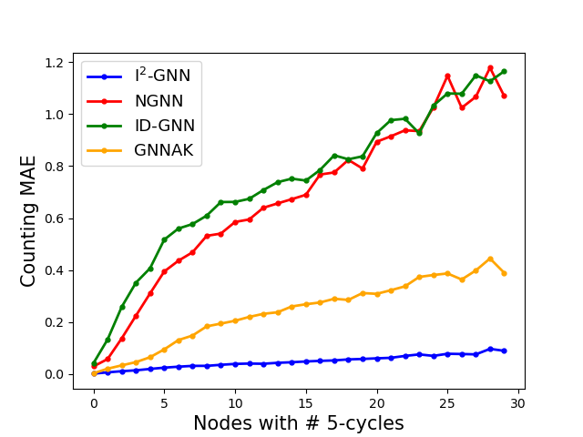
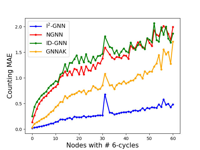
In addition, we try to understand the performance of I²-GNNs by further analysis and visualization. In subfigures (a,c) in Figure 7 we visualize the label distribution of 5-cycles and 6-cycles on synthetic dataset, i.e. nodes with different number of cycles. We see that the number of nodes with increasing cycles decays exponentially. Thus it implies the difficulty to generalize to nodes with more cycles. In the subfigures (b,d) in Figure 7 we show the corresponding prediction average MAE on nodes with different number of cycles. we can see that the MAE of Subgraph GNNs increases dramatically as the number of cycles become larger. In contrast, I²-GNNs have a almost flatten curve, implying it fits the real counting function well and thus generalizes better.

H.2 Results of counting at graph level

Using the same setup in node-level counting, we also conduct counting experiments at graph level. Note that I²-GNNs can count 6-cycles at graph level with theoretical guarantees (by Theorem 4.1), while other Subgraph GNNs are unclear. Interestingly, the experimental results in Table 9 show that all Subgraph GNNs attain comparable performance with respect to I²-GNNs and PPGNs. It may be because: (1) they capture some statistical biases that are highly correlated to graph-level counting functions; (2) they can count up to $6$ -cycles at graph level theoretically. The graph-level counting power of Subgraph GNNs is unclear from $5$ -cycles to $7$ -cycles and worthy exploring in the future research.

Table 9: Normalized MAE results with errors of counting substructures at graph level. The reported uncertainty is one times standard deviation.

Method	Synthetic (norm. MAE)
Method	3-Cycle	4-Cycle	5-Cycle	6-Cycle
GatedGCN	$0.3845\!\pm\!0.0057$	$0.2481\!\pm\!0.0010$	$0.1849\!\pm\!0.0014$	$0.1500\!\pm\!0.0036$
ID-GNN	$0.0008\!\pm\!0.0005$	$0.0064\!\pm\!0.0001$	$0.0070\!\pm\!0.0010$	$0.0182\!\pm\!0.0010$
NGNN	$0.0009\!\pm\!0.0002$	$0.0054\!\pm\!0.0005$	$0.0077\!\pm\!0.0026$	$0.0249\!\pm\!0.0010$
GNNAK+	$0.0021\!\pm\!0.0004$	$0.0177\!\pm\!0.0026$	$0.0233\!\pm\!0.0022$	$0.0412\!\pm\!0.0025$
PPGN	$0.0013\!\pm\!0.0007$	$0.0050\!\pm\!0.0005$	$0.0123\!\pm\!0.0013$	$0.0159\!\pm\!0.0015$
I²-GNN	$0.0010\!\pm\!0.0001$	$0.0066\!\pm\!0.0011$	$0.0098\!\pm\!0.0005$	$0.0237\!\pm\!0.0011$

Appendix I Ablation Study

In ablation study, we focus on studying the impact of the key element of I²-GNNs: the additional identifiers. Concretely, let $i$ be the root node and $j$ be the branching node (neighbor of $i$ ), we drop all the node labeling concerning $j$ in the subgraph $G_{i,j}$ . It results in a model denoted I²-GNNs (single) with only one identifier and all other hyper-parameters unchanged. In additional, we also study the effect of the shortest path labeling v.s. identity labeling. We implement I²-GNNs (id), where the shortest path labelings $z_{i,j,k}=\text{spd}(i,k)\oplus\text{spd}(j,k)$ are replaced with the identity labeling $z_{i,j,k}=\mathbbm{1}_{i=k}\oplus\mathbbm{1}_{j=k}$ .

Table 10: Ablation study on single node labeling and identity labeling. The reported uncertainty is one times standard deviation.

Dataset/Task	I²-GNNs	I²-GNNs (single)	I²-GNNs (id)
3-Cycle	$0.0003\!\pm\!0.0000$	$0.0004\!\pm\!0.0002$	$0.0003\!\pm\!0.0001$
4-Cycle	$0.0015\!\pm\!0.0001$	$0.0021\!\pm\!0.0001$	$0.0015\!\pm\!0.0001$
5-Cycle	$0.0028\!\pm\!0.0001$	$0.0426\!\pm\!0.0005$	$0.0034\!\pm\!0.0000$
6-Cycle	$0.0078\!\pm\!0.0007$	$0.0465\!\pm\!0.0009$	$0.0103\!\pm\!0.0021$
4-Clqiue	$0.0003\!\pm\!0.0001$	$0.0604\!\pm\!0.0902$	$0.0012\!\pm\!0.0014$
4-Path	$0.0041\!\pm\!0.0010$	$0.0241\!\pm\!0.0007$	$0.0019\!\pm\!0.0001$
Triangle-Rectangle	$0.0026\!\pm 0.0002$	$0.0566\!\pm\!0.0015$	$0.0017\!\pm\!0.0001$

From Table 10 we can see that performance drops greatly for $5,6$ -cycles, $4$ -cliques, $4$ -paths and triangle-rectangle after removing the additional identifiers. This is consistent to our claim that the additional identifiers do boost the counting power. In the comparison between shortest path labeling and identity labeling, we can see that they do not dominate each other. This is because they have the same representational power and thus the results should depend on the inductive bias of the task.

Appendix J Discussion on complexity

J.1 Comparison to other GNN models

I²-GNNs increase the representational power by extending Subgraph MPNNs (single identifier) to a pair of identifiers. In the language of equivariant tensors, I²-GNNs lift the original graph (adjacency matrix, 2-order tensor) to a 4-order tensor (first two indices for the two identifiers, last two indices for adjacency), and perform message passing on this 4-order tensor. Thus one should expect I²-GNNs’ power to be upper bounded by 4-IGN/4-WL, as implied in [9]. Regarding the complexity, suppose a graph has $N$ nodes with average node degree $d$ , and the maximum subgraph size is set to $s$ . One layer message passing takes $\mathcal{O}(d)$ time for one node. By leveraging the sparsity of graphs, I²-GNNs reach a linear time complexity $\mathcal{O}(Nsd^{2})$ w.r.t. node number $N$ . Specifically, counting 6-cycles only requires extracting 3-hop rooted subgraphs, resulting in $\mathcal{O}(Nd^{5})$ complexity. Note that in molecule datasets the node degree is usually small (e.g., QM9 has an average node degree $2.1$ ), which makes the computation feasible. This is in contrast to the at least $\mathcal{O}(N^{3})$ complexity of those high-order GNNs such as PPGNs [6] and $k$ -IGNs [13]. Some works also try to design localized high-order GNNs. For example, $k$ -GNNs [5] and $\delta$ - $k$ -LGNNs [16] reduce the time complexity to linear by constraining the $k$ -tuples to be connected and aggregating messages from neighbors only. Compared to them, I²-GNNs have an exclusive advantage: the initial features $x_{i,j,k}$ can be augmented with some three-tuple attributes, such as $x_{i,j,k}=(\text{spd}(i,k),\text{spd}(j,k))$ or other structural/positional encodings. Besides, I²-GNNs have provable substructure counting power. Local relational pooling [19] is a universal approximator for permutation invariant functions over subgraphs, but the $\mathcal{O}(Ns!)$ complexity is almost infeasible. A contemporary work [67] also discusses the possibility of high-order Subgraph GNNs: they propose to tie each subgraph with a $k$ -tuple. However, their main focus is the theoretical comparison with $k$ -WL test. Besides, the complexity of their original model grows exponentially.

Table 11: Space and time complexity of different GNN models.

Model	MPNN	Subgraph MPNN	I²-GNN	PPGN	1-2-3 GNN
Space complexity	$\mathcal{O}(N)$	$\mathcal{O}(Ns)$	$\mathcal{O}(Nsd)$	$\mathcal{O}(N^{2})$	$\mathcal{O}(Nd^{2})$
Time complexity	$\mathcal{O}(Nd)$	$\mathcal{O}(Nsd)$	$\mathcal{O}(Nsd^{2})$	$\mathcal{O}(N^{3})$	$\mathcal{O}(Nd^{3})$

J.2 Empirical complexity evaluation

Table 12: Empirical evaluation of complexity of I²-GNNs, Subgraph GNNs and PPGNs.

Model	MPNN	ID-GNN	NGNN	GNNAK+	I²-GNN	PPGN
$\#$ Parms	27k	102k	127k	251k	143k	96k
Memory usage (GB)	1.88	2.35	2.34	2.35	3.59	2.30
Inference time (ms)	2.10	5.73	6.03	16.07	20.62	35.33

We empirically compare the models’ complexity through: (1) number of parameters ( $\#$ Parms); (2) Maximal GPU memory usage (Max. memory usage) and (3) inference time. We adopt node-level counting task. The model implementation is exactly the same as in F.1, except that PPGN’s embedding size is adjusted to 64 for a fair comparison. Batch size is 256, and we run 10 epochs to compute the average inference time per batch and the maximal memoery usage during inference. We use thop package to estimate the number of parameters. Note that in the realizations of listed Subgraph GNNs and I²-GNNs, the subgraph extraction is preprocessed and thus the forward computation is in parallel. This causes a greater memory usage but a faster speed of training/inference.

From the Table 12 we can see that the inference time of I²-GNNs is feasible, since the average node degree of counting dataset is approximately 3.3.

Appendix K Scaling up: branch node sampling

Like Subgraph MPNNs, the extracted $K$ -hop ego-networks size in I²-GNNs is $\mathcal{O}(d^{K})$ . In addition, compared to Subgraph MPNNs, I²-GNNs further increase the complexity by a factor of node degree $d$ . In case where average node degree is large or the node degree distribution is heavy-tailed, the computational cost might still be unfordable.

Table 13: Statistics of the selected datasets from TUD benchmark.

Dataset	#Graphs	Avg. #Nodes	Avg. #Edges
ENZYMES	600	32.6	62.1
IMDB-BINARY	1,000	19.8	96.5

One can apply any subgraph sampling strategy to address the growing subgraph size problem, as the one in [29]. Here we focus on alleviate the growing branch node problem. We provide a simple but effective sampling strategy: randomly sample a fixed number of branch nodes to bound the additional factor by a constant. The sampling are only applied to training process, and thus permutational equivariance still holds during test.

Table 14: Test accuracy (%) with one standard deviation on TUD benchmark. I²-GNN-sample refers to I²-GNNs that randomly choose and fix two branch nodes to label before training.

Datasets	Base GNN	Nested GNN	I²-GNN	I²-GNN-sample
ENZYMES	27.3±7.8	31.7±3.7	35.8±7.1	33.8±5.9
IMDB-BINARY	70.2±5.1	71.4±5.9	73.5±3.0	72.7±3.9

Table 15: #parameters / training time per 200 epochs (s) / inference time per epoch (ms) on TUD benchmark. Training/inference time are estimated on full dataset.

Datasets	Base GNN	Nested GNN	I²-GNN	I²-sample-GNN
ENZYMES	24k/19.45/59.09	25k/30.31/107.44	34k/62.82/213.44	34k/45.68/213.03
IMDB-BINARY	24k/31.19/88.49	25k/65.28/238.91	34k/355.98/1273.30	34k/100.33/1270.62

Formally, let $N(i)$ be the neighbor of root node $i$ . An I²-sample-GNN has the same architecture with I²-GNN during training, except that

•

in equation (6), the branch node $j$ iterates over $\text{Sample}_{S}(N(i))$ instead of $N(i)$ , where $\text{Sample}_{S}$ is a sampling function that randomly chooses $S$ elements from the multiset.
•

in equation (8), the node read-out function becomes

$\forall i\in V,\quad h_{i}=\alpha_{i}\cdot R_{\text{node}}(\{h_{i,j}|j\in\text{Sample}_{S}(N(i))\}),$ (32)

where $\alpha_{i}=\frac{d_{i}}{S}$ if $R_{\text{node}}$ is additive to node degree $d_{i}$ (such as sum pooling), and $\alpha_{i}=1$ if $R_{\text{node}}$ is independent of node degree $d_{i}$ (such as average pooling).

On the other hand, sampling is disabled when doing inference in order to assure permutational equivariance, i.e. I²-sample-GNN use the exactly same architecture with I²-GNN during inference. Note that because of the stochastic branch node sampling, I²-sample-GNN would not be able to learn exact counting function. Instead it approximates the counting function in an expectational meaning.

To test the effectiveness of branch node sampling, we choose some high-node-degree datasets from TUD benchmark [77]. Table 13 above shows the dataset statics. We randomly choose and fix two branch nodes for each root node before training. The sampling does not apply to testing. We compare performance of I²-GNNs with branch node sampling to that of original I²-GNNs, base GNN (4-layer GraphConv) and Nested GNN. The subgraph depth is $3$ for ENZYMES and $2$ for IMDB-BINARY. We train each model for 200 epochs, with initial learning rate $0.002$ and decay rate $0.5$ per 50 epochs. We report the 10-fold cross validation results in Table 14. It demonstrates that I²-GNNs with even simple branch node sampling still can bring improvements to baselines and achieve competitive performance to original I²-GNNs.

Moreover, we compare the number of parameters, the training/test time for these models, as shown in Table 15. As we expected, I²-sample-GNN can significantly reduce the training time, especially for high-node-degree dataset IMDB-BINARY.

Boosting the Cycle Counting Power of Graph Neural Networks with I2-GNNs

Abstract

1 Introduction

2 Preliminaries

Definition 2.1 (Graph-level counting).

Definition 2.2 (Node-level counting).

3 Counting power of MPNNs and Subgraph MPNNs

3.1 Counting power of MPNNs

Remark 3.1.

3.2 Counting power of Subgraph MPNNs

Definition 3.1 (Subgraph MPNNs).

Proposition 3.1.

Theorem 3.1.

Theorem 3.2.

4 I2-GNNs

Proposition 4.1.

Theorem 4.1.

Theorem 4.2.

Theorem 4.3.

5 Related Works

6 Experiments

6.1 Discriminating non-isomorphic graphs

6.2 Graph substructure counting

6.3 Molecular properties prediction

7 Conclusion

8 Acknowledge

References

Appendix A Weisfeiler-Lehman test

Appendix B Counting power of MPNNs

Theorem B.1.

Proof.

Theorem B.2.

Proof.

Appendix C Discussion on Proposition 2 in [8]

Appendix D Counting power of Subgraph MPNNs

Lemma D.1 (Identity labeling is the most powerful strategy).

Proof.

Lemma D.2.

Proof.

D.1 Proof of Proposition 3.1

D.2 Proof of Theorem 3.1

D.3 Proof of Theorem 3.2

Appendix E Counting power of I2-GNNs

Lemma E.1.

Proof sketch.

Proof.

E.1 Proof of Proposition 4.1

E.2 Proof of Theorem 4.2

E.3 Proof of Theorem 4.1

E.4 Proof of Theorem 4.3

E.5 Some other graphlets

Appendix F Additional details of the numerical experiments

F.1 Graph structures counting

F.2 Molecular properties prediction

F.2.1 QM9

F.2.2 ZINC

F.2.3 OGB

Appendix G Cycles statistics on datasets

Appendix H More about counting experiments

H.1 Counting error versus number of cycles

H.2 Results of counting at graph level

Appendix I Ablation Study

Appendix J Discussion on complexity

J.1 Comparison to other GNN models

J.2 Empirical complexity evaluation

Appendix K Scaling up: branch node sampling

Boosting the Cycle Counting Power of Graph Neural Networks with I²-GNNs

4 I²-GNNs

Appendix E Counting power of I²-GNNs