FocusedCleaner: Sanitizing Poisoned Graphs
for Robust GNN-based Node Classification
Abstract
Graph Neural Networks (GNNs) are vulnerable to data poisoning attacks, which will generate a poisoned graph as the input to the GNN models. We present FocusedCleaner as a poisoned graph sanitizer to effectively identify the poison injected by attackers. Specifically, FocusedCleaner provides a sanitation framework consisting of two modules: bi-level structural learning and victim node detection. In particular, the structural learning module will reverse the attack process to steadily sanitize the graph while the detection module provides the “focus” – a narrowed and more accurate search region – to structural learning. These two modules will operate in iterations and reinforce each other to sanitize a poisoned graph step by step. As an important application, we show that the adversarial robustness of GNNs trained over the sanitized graph for the node classification task is significantly improved. Extensive experiments demonstrate that FocusedCleaner outperforms the state-of-the-art baselines both on poisoned graph sanitation and improving robustness.
Index Terms:
Graph Learning and Mining, Graph Adversarial Robustness, Discrete Optimization, Victim Node DetectionI Introduction
In the past few years, Graph Neural Networks (GNNs) are potent deep learning models to capture semantic and structural information of the relational data for widely-adopted downstream tasks such as node classification [1, 2], link prediction [3], community detection [4], graph classification [5] and graph anomaly detection [6] due to their specially-designed aggregation mechanism. The aggregation mechanism can propagate the node’s features along the topology on the non-Euclidean space and obtain the node representations with good quality. However, extensive research efforts have been devoted to studying the robustness of GNNs under attack and verifying that GNNs are prone to be attacked by imperceptible structural attacks [7, 8]. In particular, a prevalent type of attack, termed data poisoning attack [9], studies how to manipulate the input graph data (especially the graph structure) to mislead GNNs’ predictions. Basically, an attacker can tamper with the data collection process to create a poisoned graph, over which an analyst runs GNN-based prediction algorithms that would make possibly wrong predictions. Such poisoning attacks are shown to be very effective in various graph analytic tasks [7, 8, 10].
Against this background, we are thus motivated to investigate this important problem of poisoned graph sanitation: given a poisoned graph, how can the analyst (defender) identify the poison injected by the attacker? This problem is important for a few reasons. First, unlike attacks over images where the poison is meaningless noise, poison over graphs (e.g., edges and nodes) often possess some physical meanings. Thus, identifying the poison itself could be useful. For example, consider a poisoning attack against a recommendation system [11] where the attacker modifies the user-item bipartite graph. The poison injected by the attacker corresponds to the actual reviews, the successful identification of which could help to locate the fake/compromised user accounts and further trace the attacker. Second, data sanitation can act as a data preprocessing step, which can serve as an important defense mechanism – indeed, we demonstrate that our sanitation techniques can greatly enhance the robustness of GNN-based node classification. In this paper, we focus on sanitizing the structural noise (i.e., edges) introduced by attackers.
Graph sanitation problem resembles a well-investigated topic termed graph structural learning. Specifically, given a graph contaminated by noise (could be random or adversarial), graph structural learning aims to introduce some slight refinement to the graph structure (thus learning a new graph ) in the hope that the refinement can “neutralize” the effects of the noise so as to improve model performance. For instance, a representative line of research applies data augmentation techniques [12, 13, 14] to boost the node classification accuracy of GNNs. In particular, the work closely related to ours is GASOLINE [14], which utilizes a bi-level structural learning framework to search for a “better” topology to increase node classification accuracy. However, we emphasize that structural learning and data sanitation have very distinct goals. The formal aims to improve model performance by learning a new graph with no intention to recover the original clean graph . In comparison, sanitation explicitly aims to identify and remove the poison to recover , and importantly a natural result of sanitation is improved model performance. We elaborate on this key difference with supporting experiment results in Section VI-A.
To tackle the problem of poisoned graph sanitation, we present FocusedCleaner, a framework composed of two modules: a bi-level structural learning module and a victim node detection module. Importantly, these two modules will operate collaboratively to enhance each other. On the one hand, the detection module acts as a supervisor and provides the “focus” to narrow down the search region for the structural learning module, which can more accurately pick out the adversarial links. On the other hand, the inner training component of the structural learning module can learn node features with higher quality, which boosts the performance of the detection module. Overall, these two modules will reinforce each other and provide better sanitation results.
The application of FocusedCleaner to enhance the adversarial robustness of GNN-based node classification is immediate: GNN models trained over the sanitized graph can achieve much better performance. That is, FocusedCleaner can effectively serve as a preprocessing-based defense approach against data poisoning attacks.
In summary, we propose a poisoned graph sanitizer FocusedCleaner that possesses the following nice features:
- •
FocusedCleaner can achieve better sanitation performance than state-of-the-art baseline approaches in terms of effectively identifying the attacker-injected edges in a poisoned graph to recover the clean graph.
- •
To effectively validate the poisoned graph sanitation performance of the preprocessing-based defense methods, we introduce a rational metric– based on the Jaccard index [15]. Higher will probably lead to better robustness for node classification. Sanitation evaluation based on a traditional metric like score is also given and achieve the consistent performance with .
- •
GNN models trained over graphs sanitized by FocusedCleaner have higher node classification accuracy compared to training over graphs sanitized by other graph structural learning methods. That is, FocusedCleaner can provide better defense performance.
- •
As a preprocessing-based defense approach, FocusedCleaner outperforms state-of-the-art robust GNN models. Moreover, FocusedCleaner can also be used in combination with robust GNN models, further boosting defense performance.
II Related Works
II-A Graph Structural Learning
Graph structural learning aims to learn a slightly different graph topology to boost the performance of a specific graph learning task, such as node classification [1, 2], link prediction [3], community detection [4], etc. They assume the initially given graph has been contaminated by the noisy links or nodes, and aim at mining the topology of the graph for better downstream tasks’ performances. For example, [12] utilizes the GVAE [16] to prune the inter-cluster links and insert the intra-cluster links and train the GNN with the refined graph. [13] augment the graph locally by sampling neighbors’ GNN features to prevent the degenerated performance of the aggregation mechanism when the number of neighbors is limited. [17] augments the graph’s topology information by MH algorithm [18] which can well capture the distribution of the graph structure. [19] removes the weak links and enhances real connections to the biological networks by using a doubly stochastic matrix operator and increasing the spectrum eigengap of the input graph. [20] iteratively trains the min-cut loss [21] and GVAE and removes the irrelevant edges. [22] leverages the mutual influence of noisy links detection and missing links prediction to enhance each other. All the above methods endeavor to find a better graph structure to enhance the performance of the downstream tasks.
II-B Graph Defense
Graph defense methods aim at defending against structural poisoning or evasion attacks on the graph data and try to preserve the node classification performance under varying attacking powers. It contains two types: preprocessing-based methods and robust models. For preprocessing-based methods, [23] utilizes the Jaccard similarity to prune the potential adversarial links. [14] implements a bi-level optimization to enhance the robustness of GNN. For robust models, [24] learns a Gaussian distribution on node features and prunes the nodes with large variance. [25] adopted the cosine similarity between two nodes’ GNN features and obtain the link dropout probability during training. [26] constructed a kNN graph based on node attributes and incorporate the kNN graph into GNN to ensure attribute consistency. [27] dedicated to mitigating the influence of bad propagation by introducing robust statistics. [28] implemented the -norm to the graph signal estimator to enhance the robustness of the model. [29] introduced an adaptive residual mechanism to mitigate the abnormal node features’ impact.
III Preliminaries
III-A Notations
In this section, we first introduce the frequently used notations in Tab. I. Next, we give a brief introduction to graph neural network and structural poisoning attack.
| Notations | Descriptions |
|---|---|
| node number | |
| link set of the graph | |
| Given poisoned graph | |
| A sanitized graph recovered from | |
| Adjacency matrix of a poisoned graph | |
| Nodal attributes matrix of a graph | |
| Degree matrix of a poisoned graph | |
| Budget of the attacker | |
| Learnable weight matrix of GNN | |
| Label matrix of a graph | |
| Victim nodes set | |
| Normal nodes set | |
| Laplacian matrix of a poisoned graph | |
| relative importance of the validation loss | |
| relative importance of the testing loss | |
| output of a two-layered GNN |
III-B GNN-Based Node Classification
We frame the problem of graph data sanitization in the context of semi-supervised node classification. Specifically, denote a graph as , where / are the sets of labeled/unlabeled nodes, denotes the set of available node labels, is the attribute matrix and is the adjacent matrix. A GNN model [1] denoted as then can be trained to predict the missing node labels, where summarizes the trainable model parameters, is a finite set of labels, is the predicted label for a node in . While there are various GNN models, a typical construction of the GNN layers [1] is as follows:
| (1) |
where is the degree matrix, is the node features for -th layer, is the GNN parameters, is the adjacency matrix with self-loop. Then, GNN feeds the node features at the last layer to the NLL loss for training.
III-C Structural Poisoning Attacks
We restrict our attention to structural poisoning attacks [7] since recent results [23] show that modifying the topology is more harmful than modifying attributes. Alternatively, the semi-supervised nature of GNN is particularly suitable for the attacker to inject the poisons to the graph during the GNN training step [7]. Specifically, given a clean graph , the attacker modifies the structure (i.e., ) of the graph by inserting/removing edges, resulting in a poisoned graph . Various attack methods are proposed to find the poisoned graph such that when a GNN model is trained over , the prediction accuracy on the unlabeled nodes is minimized. The representative structural poisoning attacks are METTACK [7] and MinMax [8], which formulates the attack as a discrete bi-level optimization problem. METTACK tackles this problem by greedily searching for the largest meta-gradient of all possible node pairs to “flip” (insert or remove links) until reaches the budget. MinMax relaxes the discrete parameters to the continuous space and optimizes the problem via projection gradient descent [30] and obtain the poisoned graph by random sampling.
IV Empirical Study of Sanitation
In this section, we present an empirical study to illustrate the relationship between the poisoned graph sanitation performance and the robustness of GNN. In the meanwhile, we give a detailed description of the new metric–Effective Sanitation Ratio () and utilize this metric to quantify the quality of the sanitized graph.
It is natural that pruning the injected adversarial links in the poisoned graph will drastically boost the node classification performance of GNN (METTACK and MinMax tend to insert links rather than delete links [23]). To verify this issue, we utilize METTACK to manipulate the Cora dataset with attacking power, i.e., the graph attacker can perturb the Cora dataset at most times. It is observed that the attacker injects adversarial links and deletes links. To validate the effectiveness of pruning the adversarial links, we delete the adversarial links in the poisoned graph one by one and report the mean testing accuracy over runs of GNN after each pruning. The trace plot of the mean accuracy for each pruning is depicted in Fig. 2. The orange line is the mean accuracy of the GNN trained on the clean graph. Fig. 2 demonstrates that pruning more adversarial links in the poisoned graph will increase the performance of GNN until reaching the accuracy of the clean graph with slight deviations.
This phenomenon inspires us that under a fixed budget, a graph sanitizer’s goal is to prune the adversarial links as much as possible to recover the poisoned graph to be similar to the clean graph. As a consequence, the sanitized graph will reach a more robust performance compared with the poisoned graph. To precisely quantify the number of adversarial links successfully pruned by the graph sanitizer, we design the metric as:
| (2) |
where is the pruned links set and is the adversarial links set. Naturally, a large means most of the pruned links by the graph sanitizer are adversarial links. Moreover, we also introduce the score to quantify the sanitation performance as a reference to , i.e.,
| (3) |
To validate the effectiveness of and score, we deploy another experiment on Cora dataset with random pruning. Under the attacking power, we restrict the attacker to randomly select of the attack budget to prune the true adversarial links while the remaining budget to prune the normal links. We then report the , score and the mean node classification accuracy over runs in Fig. 3.
The experiment results demonstrate that higher and score can lead to better node classification accuracy of GNN. Specially, when and are , the poisoned graph’s accuracy is almost the same as clean graph. These phenomenons verify that a sanitized graph with good quality should have relatively high and score. From this perspective, an excellent graph sanitizer aims at sanitizing the poisoned graph to obtain a sanitized graph with high or values.
V Problem of Graph Sanitation
Now, the task of graph data sanitization is clear: a defender will try to identify the edges inserted/removed by the attacker from the poisoned graph . We denote as the sanitation made to the adjacent matrix of and assume that , meaning that the amount of sanitation (i.e., number of added and/or deleted edges) is bounded by . That is, through sanitization, the defender will obtain a sanitized graph denoted as , here denotes the sanitation operation at a high level. Then, the problem of graph sanitization can be formulated as the following optimization problem:
| (4) |
where denotes a distance metric on the adjacent matrix at a high level. In words, the defender aims to clean the poisoned graph so as to obtain a sanitized graph that is similar to the original clean graph . We follow the semi-supervised node classification setting where the defender knows a subset of node labels. We note that is the common knowledge available to both the attacker and the defender, while the ground-truth graph is only available to the attacker.
VI Poisoned Graph Sanitizer:
VI-A Importance of “Focus” for Sanitation
We explain our intuitions behind designing FocusedCleaner by discussing the limitations of the prior work GASOLINE [14] in sanitation. At a high level, instead of solving Problem (4), GASOLINE learns a new graph that could best restore the prediction accuracy from the poisoned graph. However, GASOLINE has its own bottlenecks. Our first observation is that previous studies [23, 31] have demonstrated that in structural poisoning attacks the majority of manipulations are edge insertions rather than edge deletions. This is a result of the optimization process to maximize attack performance. Thus, it is natural to restrict a sanitizer from “flipping” (both inserting and deleting) edges to deleting edges only in a poisoned graph. Based on this, we consider a variation termed GASOLINE-D, which will only delete edges.
| Methods | (%) | accuracy (%) |
|---|---|---|
| GASOLINE | ||
| GASOLINE-D |
We then compare the performance of GASOLINE and GASOLINE-D in sanitizing the poisoned graph (Cora dataset) produced by METTACK. We note that METTACK is not restricted to inserting edges only. We use the metric (defined in Eqn. (2)) to measure the quality of sanitization, where a higher means that more poisoned edges are pruned from the graph. Tab. II shows the effective sanitation ratios as well as the node classification accuracy of GNN over the sanitized graph using two methods, respectively.
There are a few crucial observations. First, GASOLINE also tends to insert edges (similar to attack) to best restore classification accuracy. This indeed shows that data sanitation is different from graph structural learning as GASOLINE has a zero recovery ratio. Second, GASOLINE-D outperforms GASOLINE in sanitation. Because by restricting to deleting edges only, GASOLINE-D narrows the search space of the meta-gradients (which are used to determine which edges to be modified first) from down to . That is, we created a more “focused” candidate space for the sanitizer to identify maliciously modified edges. This inspired us to make the candidate space more focused to improve the sanitization performance. That is the “focus” in FocusedCleaner. In addition, the fact that GASOLINE-D outperforms GASOLINE in classification accuracy provides an interesting hypothesis: recovering the clean graph might be more effective in restoring model performance than structural learning.
VI-B Framework and Overview
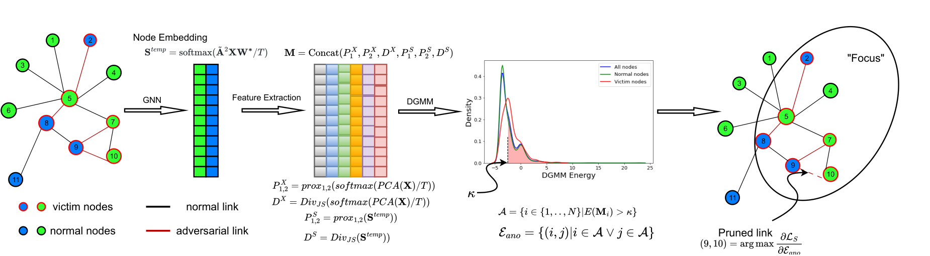
We are now ready to present FocusedCleaner (whose framework is shown in Fig. 1) consisting of two modules: bi-level structural learning and victim node detection.
We follow and improve the idea of structural learning (also used in GASOLINE) to solve the sanitation problem (4), which is impossible to solve directly since the clean graph is unknown to the defender. At a high level, we aim to find a better graph structure from which GNNs will make fewer erroneous predictions; however, we integrate a victim node detection module that will restrict the region of updates in the graph. Specifically, we reformulate the sanitation problem as the following (somehow high-level) bi-level optimization problem:
| (5a) | ||||
| s.t. | (5b) | |||
| (5c) | ||||
where and are the losses for structure learning and training the GNN model, respectively. is the initially observed poisoned graph and we treat as the optimization variables. Importantly, denotes the victim node detection module that will predict the normal node set and victim node set . Then and will provide guidance to structure learning through two aspects. First, the victim node set defines a candidate search region , which is the set of edges incident to at least one victim node in . is crucial when deciding which edges to clean. Specifically, we adopt a greedy strategy to solve the structure learning problem. That is, we compute the gradient of with respect to each edge and pick to edge corresponding to the largest gradient to clean. Second, when calculating the loss over the nodes, we make the restriction that those nodes should belong to the normal node set . We show that this strategy (compared to also calculating losses over victim nodes) could improve sanitation performance in the ablation study. We note that the optimization problem omitted some details for easier illustration of the interaction between structure learning and victim node detection; the detailed construction is presented in Section VI-C.
Overall, the victim node detection module provides two kinds of “focus” for the structural learning process. First, it restricts the loss to be calculated only over normal nodes. Second, it provides a reduced search region for identifying malicious edges. In return, the structure learning will provide a steadily sanitized graph for victim node detection, resulting in more accurate identification of victim nodes.
Next, we detail our realizations of the structural learning and victim node detection modules.
VI-C Improved Bi-level Structure Learning Module
We present the structure learning module without involving victim node detection for the moment. The typical bi-level structure learning consists of two optimization processes: GNN training (inner optimization in Eqn. 5b) and poisoned edge selection (outer optimization in Eqn. 5a). We made a few improvements to the typical structure learning module to boost sanitation performance.
First, we introduce an attribute smoother [32] to the outer optimization, serving as a regularizer to preserve high-level graph homophily. Second, we also bring in an adaptive testing loss trick (detailed later) to the outer optimization process to augment more information thus better guiding the poisoned edge selector. Moreover, we only consider the normal unlabeled nodes for calculating the loss to prevent the contaminated entropy caused by the victim nodes. Specifically, we formulate the bi-level structure learning as follows:
| (6a) | ||||
| s.t. | (6b) | |||
| (6c) | ||||
| (6d) | ||||
| (6e) | ||||
where , is the normalized adjacency matrix, is the sanitized graph, is the initial poisoned graph, is the output of the two-layered linearized GNN [33, 7], is the attribute smoother. We note that and denote the true label and the estimated label for nodes in the validation and test set, respectively. and determine the relative importance of the validation loss and testing loss in the outer optimization (Eqn. (6a)). Since the testing loss is highly skewed due to the adversarial noise in the early stage, we adaptively assign at -th sanitation step. As a result, we can adaptively let the outer loss (Eqn. (6a)) to partially pay attention to the testing loss for each sanitation step in an ascending manner. The intuition is that at the beginning we only focus on the validation loss; as the poisoned graph is sanitized step by step, we pay more attention to the testing set to augment more information to guide the cleaner.
VI-D Victim Node Detection Module
We define a victim node as a node whose incident edges/non-edges have been manipulated by the attacker. We design a victim node detection module based on two unsupervised methods termed ClassDiv and LinkPred, respectively.
VI-D1 ClassDiv Detector
Our basic idea is to identify some proper metrics that capture the difference between victim nodes and other normal nodes, and then use these metrics as input features to train an unsupervised model.
Intuitively, structural poisoning attacks against GNNs will break the homophily [34] of the graph, i.e., similar nodes tend to be interconnected. As a result, a victim node would tend to be different from its neighbors since an attacker may add an edge to connect it with a very different node or delete an edge between it and a similar neighbor. In light of this, we choose three metrics , [35] and [36] to measure how different a node is from its neighbors without loss of generality. Specifically, the three metrics utilize the logits of nodes, denoted as , given by an inner trained GNN model in Eqn. (6b) to compute the measure of difference.
We build an unsupervised Deep Gaussian Mixture Model [37] (DGMM) based on carefully designed features. First, we define the soft class probability [38] as
| (7) |
where is the temperature to be tuned. We denote . Adjusting will lead to different scales of class information and amplify the class divergence between a victim node and its neighbors or decrease the class divergence between a normal node and its neighbors. Second, we increase the efficiency of computing these metrics by vectorization technique. Specifically, we first define the pairwise KL divergence [39]:
Definition 1.
Let be the output of the pre-trained GNN, the pairwise softmax KL divergence is defined as:
| (8a) | ||||
| (8b) | ||||
| (8c) | ||||
Here represents the element-wise product of two matrices. We thus can reformulate and by the defined pairwise softmax KL divergence:
Definition 2.
Let be the pairwise KL divergence based on the output of GNN, and are formulated as:
| (9) | ||||
| (10) |
Proof.
∎
Third, we construct the input features for DGMM as:
| (11a) | ||||
| (11b) | ||||
| (11c) | ||||
| (11d) | ||||
| (11e) | ||||
where is the input features that distill the class divergence information for each node. We use PCA [40] to reduce the attributes dimension to the class number . It is worth noting that if the graph does not have attributes, we only consider . Next, we feed the hybrid features into the unsupervised DGMM [37] to identify the victim nodes as follows:
| (12a) | ||||
| (12b) | ||||
| (12c) | ||||
| (12d) | ||||
| (12e) | ||||
where denotes the probability of the node belonging to the cluster (we set equal to the class number ), is the energy function of DGMM. We adopt the Adam optimizer [41] to optimize the energy function . After training, we compute for each node and higher tend to be anomalous. For evaluation, we denote the -th quantile of the energy scores as and regard a fraction of of the nodes as the victims. However, setting a fixed value of is not a wise choice since, as the graph is sanitized, there should be fewer victim nodes. To address this, we use an adaptive threshold for victim node detection. Inspired by the momentum trick [42], we update the threshold at each sanitation step for victim node detection as:
| (13a) | ||||
| (13b) | ||||
where is the threshold for the -th sanitation step, is the -th quantile based on the energy score at -th sanitation step, is the hyperparameter to balance the quantile at -th step and the threshold at last step. Thereafter, we adaptively predict the victim node set at -th sanitation step as:
| (14) |
The remaining nodes are regarded as normal.
VI-D2 LinkPred Detector
Alternatively, we also observe that link prediction [3] can be used to detect the potential victim nodes. Intuitively, a link prediction model can assign each link a probability, and a link with a lower probability tends to be maliciously injected. We then regard a node as a victim if it is incident to a malicious link. To this end, we utilize the node embeddings output from the inner training (Eqn. (6b)) of GNN as input and build up a two-layer MLPs [43] with an inner-product layer as the prediction model (termed as LinkPred):
| (15a) | ||||
| (15b) | ||||
Similarly, we remove if the graph does not have attributes. The loss function is the reweighting binary cross-entropy loss with the reweighting parameter to tackle the imbalanced problem when training. We choose the threshold which can max the G-mean [44] of the prediction results. We then obtain the victim node set at -th sanitation step as:
| (16) |
where is the link set, is the threshold at -th step. Finally, this victim node detection module then interacts with structure learning as illustrated in Section VI-B to perform sanitation. The algorithm of is shown in Alg. 1.
Output: Sanitized graph .
VI-E Time and Space Complexity
The time complexity of involves the computation of the meta-gradients for all the node pairs and the hybrid features in Eqn. 11. By utilizing the vectorization technique for computing and , the time complexity of computing decreases from to . While it is known that the time complexity of GASOLINE [14] is , where is the average nodes degree. Since narrow down the search space from to ( is the adversarial links set), the time complexity of structural learning module is . After augmenting the victim node detection module, the time complexity of is . Similar to GASOLINE, the space complexity of is if the graph is stored as sparse matrix and for dense matrix.
VII Experiments
In this section, we evaluate the sanitation performance of FocusedCleaner and how it contributes to the robustness of GNN-based node classification and answering the following three vital questions:
- •
How is the performance of FocusedCleaner in sanitizing poisoned graphs?
- •
Is it necessary to augment the bi-level structural learning framework with victim node detection?
- •
How can FocusedCleaner contribute to the adversarial robustness of GNNs for node classification?
VII-A Experimental Settings
VII-A1 Datasets
We evaluate the methods over three standard datasets: Cora [45, 46], Citeseer, and Polblogs, where Polblogs has no node features. Since Polblogs does not have node attributes, we use the identity matrix to represent its attribute matrix. We follow the same setting as GASOLINE [14] and randomly split the datasets into training (), validation() and testing () dataset. The statistics of the datasets are presented in Tab. III. We only consider the largest connected component (LCC) [7] of each graph.
| Datasets | Classes | Features | ||
|---|---|---|---|---|
| Cora | ||||
| Citeseer | ||||
| Polblogs | / |
GCN [1] is used as the default GNN model for all the evaluations. METTACK and MinMax are employed as the two representative global structural attacks to test all the sanitation and defense methods.
VII-A2 Baseline Methods
To evaluate the sanitation performance of FocusedCleaner, we compare it with other state-of-the-art graph structure learning methods (which could also be used as sanitizers): GCN-Jaccard, maskGVAE, and GASOLINE-D (we ignore GASOLINE here since GASOLINE has been proved to be less effective than GASOLINE-D in Sec. 6.1). For a fair comparison, we restrict all these sanitizers to deleting edges only. We note that since these sanitizers can clean the poisoned data, they can act as preprocessing-based defense methods. Meanwhile, there are other robust GNN models that are designed to defend against attacks; we term them as robust-model-based defense methods. Thus, to evaluate the defense performance of FocusedCleaner, we compare it with both preprocessing-based and notable robust-model-based methods, including ProGNN [32], RGCN [24], MedianGNN [27], SimPGCN, GNNGUARD [26], ElasticGNN [28] and AirGNN [29]. We use Deeprobust [47] to implement two typical structural poisoning attack methods: METTACK and MinMax and two defense methods GNN-Jaccard [23] and ProGNN [32]. We use GreatX [48] to implement RGCN, MedianGNN, SimPGCN, GNNGUARD, ElasticGNN and AirGNN. We implement GASOLINE-D and maskGVAE using the codes provided by the authors. The descriptions of the preprocessing-based models are listed below:
- •
GCN-Jaccard It prunes links based on the nodes’ attribute similarities.
- •
maskGVAE It trains the graph partition task and adopts the clustering results to supervise the graph autoencoder.
- •
GASOLINE-D It adopts the bi-level optimization to augment the optimal graph structure by pruning links for the node classification task. It is a variant of GASOLINE.
While the description of robust GNNs are:
- •
RGCN It utilizes gaussian distributions to represent node features and assigns an attention mechanism to penalize nodes with large variance.
- •
ProGNN It jointly trains a dense adjacency matrix and the node classification with three penalties: feature smoothness, low-rank and sparsity.
- •
MedianGNN It utilizes the median aggregation layer to enhance the robustness of GNN.
- •
SimPGCN It utilizes a kNN graph to capture the node similarity and enhance the node representation of the GNN.
- •
GNNGUARD It utilizes the cosine similarity to calculate the link pruning probability during GNN training.
- •
ElasticGNN It introduces -norm to graph signal estimator and proposes elastic message passing during GNN training.
- •
AirGNN It adopts an adaptive message passing scheme to enhance GNN with adaptive residual.
The default hyperparameter settings for FocusedCleaner are: , , and . We tune from , ranged from , ranged from and ranged from . Since the Polblogs does not have node attributes, we set and remove the corresponding features . For all the defense models, we report the mean accuracy of runs with different random seeds. The dimension of the GCN hidden layer is . For METTACK and MinMax, we consider different attacking powers: , , , and based on the number of links for clean graph.
VII-B Analysis of Sanitation Performance
VII-B1 Evaluation Metric
Let and be the set of malicious edges injected by the attacker and the set of suspected malicious edges produced by a sanitizer. We define the defender’s Affordable Sanitation Budget as the ratio , where denotes the number of edges in the poisoned graph. Practically, measures how much effort the defender could afford to deal with the sanitation result . Because in practice, the defender usually needs to invest manpower to examine the found malicious edges for verification. Thus, setting a large for a sanitizer would be overloaded. We follow the baseline method GASOLINE-D to set a fixed value of throughout the evaluation (For GCN-Jaccard, we are tuning the threshold as the number of deleting links is near for the poisoned graph with different attacking powers, i.e., the threshold for Cora, Citeseer and Polblogs are , and ); later on, we also discuss the effects of on sanitation performance.
As previously mentioned in Sec. 4, we utilize two metrics and score to quantify the sanitation performance of the graph sanitizer. We select and score as the main metrics because, on the one hand, they measure how good the sanitizer is in successfully spotting malicious edges (i.e., ) and on the other hand, they prevent a sanitizer from irresponsibility output too many suspected edges (i.e., and ), thus causing lots of false alarms. Moreover, we define another metric Coverage Ratio, i.e.,
| (17) |
to measure the percentage of malicious edges that are successfully identified.
VII-B2 Sanitation Results
Since we have two different victim node detectors ClassDiv and LinkPred, we term the corresponding sanitizer as FocusedCleanerCLD and FocusedCleanerLP, respectively. We use the attacks to poison a graph with varying attack power, which is the fraction of malicious edges over all edges in the clean graph. We note that the attacks are allowed to insert and remove edges; however, we observe that more than of operations are inserting.
Fig. 4 and 5 presents the and score of different sanitizers against METTACK and MinMax under various attack powers. Note, the results of GCN-Jaccard are missing on Polblogs because this method relies on node features. It is observed that our sanitizers outperform others by a large margin in almost all cases, which demonstrates the effectiveness of the detection module in providing a focus for sanitation. Overall, FocusedCleanerCLD is slightly better than FocusedCleanerLP. We also observe that on Polblogs, our sanitizers are not as good as GASOLINE-D in some cases. The possible reason is that nodes in Polblogs have no features, which might impair the victim node detection’s performance. It is observed that scores show a similar trend as and our methods almost always outperform other baselines.
| Preprocessing-based methods | Robust models | |||||||||||||
|---|---|---|---|---|---|---|---|---|---|---|---|---|---|---|
| Dataset | Ptb rate | GCN | GCN-Jaccard | maskGVAE | GASOLINE-D | FocusedCleanerLP | FocusedCleanerCLD | RGCN | ProGNN | MedianGNN | SimPGCN | GNNGUARD | ElasticGNN | AirGNN |
| Cora | 83.6 | |||||||||||||
| 81.1 | ||||||||||||||
| 76.5 | ||||||||||||||
| 71.9 | ||||||||||||||
| 66.0 | 66.0 | |||||||||||||
| Citeseer | 74.9 | |||||||||||||
| 71.7 | ||||||||||||||
| 65.5 | ||||||||||||||
| 60.8 | ||||||||||||||
| 58.0 | ||||||||||||||
| Polblogs | 88.5 | |||||||||||||
| 88.0 | ||||||||||||||
| 86.0 | ||||||||||||||
| 78.9 | ||||||||||||||
| 72.3 | ||||||||||||||
| Preprocessing-based methods | Robust models | |||||||||||||
|---|---|---|---|---|---|---|---|---|---|---|---|---|---|---|
| Dataset | Ptb rate | GCN | GCN-Jaccard | maskGVAE | GASOLINE-D | FocusedCleanerLP | FocusedCleanerCLD | RGCN | ProGNN | MedianGNN | SimPGCN | GNNGUARD | ElasticGNN | AirGNN |
| Cora | 83.6 | |||||||||||||
| 82.9 | ||||||||||||||
| 81.8 | ||||||||||||||
| 79.6 | ||||||||||||||
| 77.4 | ||||||||||||||
| Citeseer | 74.1 | |||||||||||||
| 73.7 | ||||||||||||||
| 73.2 | ||||||||||||||
| 73.2 | ||||||||||||||
| 71.1 | ||||||||||||||
| Polblogs | 92.2 | |||||||||||||
| 90.9 | ||||||||||||||
| 90.3 | ||||||||||||||
| 66.8 | ||||||||||||||
| 69.2 | ||||||||||||||
VII-B3 Discussion on Affordable Sanitation Budget
The selection of is a practical issue. It depends on the defender’s ability to process the sanitation results as well as his prior knowledge of the attack power, i.e., the number of malicious edges expected in the poisoned graph. Thus, it is beneficial to see the effects of different levels of on sanitation performance. To this end, we vary the values of and check the performance of the sanitizer against different attack powers. We use FocusedCleanerCLD against METTACK as the example. The sanitation results () are shown in Fig. 6. In general, when matches the attack power (the diagonal entries), we can achieve the best recovery ratios. In addition, Fig. 7 shows the values of as we increase the budget . As expected, as the defender invests more (i.e., larger ), more malicious edges (over ) will be identified for all attack powers. Moreover, for a fixed attack power (i.e., a particular line in Fig. 7), the increase of will slow down as we increase , demonstrating a typical diminishing return phenomenon – it is more evident for lower attack powers (i.e., fewer injected malicious edges).


VII-C Sensitivity Analysis
FocusedCleanerCLD has some vital hyperparameters which can influence its sanitation performance, i.e., temperature in the soft class probability, hyperparameter for the momentum trick, relative importance for the attribute smoother and the fraction for computing energy score’s quantile. We present the sensitivity analysis on these four hyperparameters in Fig. 8. Fig. 8(a) shows that crafting a suitable temperature for the GNN features will lead to better recovery performance, this is due to the increasing performance of the victim node detection module. Fig. 8(b) shows that choosing the appropriate combination of the quantile at -th step and the threshold at ()-th step will lead to a more suitable threshold for the unsupervised victim node detection. Fig. 8(c) demonstrates that introducing the feature smoothness penalty to the outer loss can also improve the sanitation performance of the FocusedCleaner. Fig. 8(d) verifies that setting is the best choice for the victim node detection. This phenomenon is rational since the too-narrow search space of the sanitizer will degenerate the sanitation performance.
VII-D Ablation Study
The fact that FocusedCleaner outperforms GASOLINE-D demonstrates the importance of the victim node detection module as the “focus” in sanitation. On the other hand, to show the importance of the bi-level structure learning module, we run the following experiments. Since the LinkPred-based detection module itself can detect adversarial links, we directly use it as a sanitizer without bi-level structure learning. We implement the FocusedCleanerLP and LinkPred on Cora dataset as an exemplar. Tab. VI shows that FocusedCleanerLP outperforms LinkPred by a large margin. In combination, these results show that the structure learning and detection modules can enhance each other in the sanitation process.
| Attacking power | FocusedCleanerLP | LinkPred |
|---|---|---|
On the other hand, we also analyze the importance of the adaptive testing loss trick () for . We set to represent the ignorance of the testing loss during sanitation, and the ablation study results are shown in Tab. VII. The results demonstrate that dynamically introducing the testing loss can better supervise the cleaner to assign a higher meta-gradient to the adversarial noise, thus leading to a better sanitation performance.
| Attacking power | FocusedCleanerCLD-w. | FocusedCleanerCLD-w.o. |
|---|---|---|
Moreover, we also analyze the necessity of introducing “focus” on the structure loss by only considering the normal nodes in the validation and testing set. The results are shown in Tab. VIII. The experimental results demonstrate that introducing the “focus” into the structure learning loss indeed boosts the sanitation performance of .
| Attacking power | FocusedCleanerCLD-w. | FocusedCleanerCLD-w.o. |
|---|---|---|
VII-E Sanitation for Robust Node Classification
We proceed to evaluate FocusedCleaner as a preprocessing-based defense method and compare it to other defense approaches (both preprocessing-based and robust-model-based). For preprocessing-based methods, we test GCN on the sanitized graph. For robust-model-based methods, we directly feed the poisoned graph to the robust models. Table IV and Table V summarize the node classification accuracies under different attack powers. Among all the methods, our proposed FocusedCleanerCLD and FocusedCleanerLP can achieve the best results in almost all cases, even outperforming robust-model-based methods. This shows that correctly eliminating the adversarial links might be a potentially better choice than mitigating the impairments of adversarial noises. Besides, the consistency between the recovery ratio and the robustness performances shows that robustness is indeed a result of sanitation.
We note that preprocessing-based and robust-model-based methods are two complementary defense approaches rather than conflicting. Indeed, we can feed the sanitized graph into the robust models, and we can observe a further performance boost. We show such results in the Sec. I of the supplement.
VII-F FocusedCleaner with Robust Models
The two types of defense approaches are not conflicting with each other but are rather complementary. That is, we can use preprocessing-based methods to sanitize the graph and then feed the graph into robust models. Specifically, we use MedianGNN and ElasticGNN as two representative robust models. Tab. IX and Tab. X show the node classification accuracies with/without the sanitation step. Indeed, sanitation will enhance the performance of robust models as sanitized graphs will have a higher level of homophily compared with poisoned graphs.
| Dataset | Attacking power | MedianGNN-w. | MedianGNN-w.o. | ElasticGNN-w. | ElasticGNN-w.o. |
|---|---|---|---|---|---|
| Cora | |||||
| Citeseer | |||||
| Polblogs | |||||
| Dataset | Ptb rate (%) | MedianGNN-w. | MedianGNN-w.o. | ElasticGNN-w. | ElasticGNN-w.o. |
|---|---|---|---|---|---|
| Cora | |||||
| Citeseer | |||||
| Polblogs | |||||
VIII Conclusion
In this paper, we target on the graph sanitation problem which aims at pruning the maliciously adversarial links from the poisoned graph. In particular, we propose a new framework–FocusedCleaner to joint learn a bi-level structure learning module with a crafted unsupervised victim node detection module. Specially, the victim node detection module provide the “focus” to help the structure learning module precisely identify and prune the candidate adversarial links. To validate the sanitation performance, we design a new metric– based on the Jaccard index to scientifically measure the sanitation quality. The experimental results demonstrate that our sanitizers achieve comparable performances both on graph sanitation and graph defense task.
References
- [1] T. N. Kipf and M. Welling, “Semi-supervised classification with graph convolutional networks,” in International Conference on Learning Representations, 2017.
- [2] W. Hamilton, Z. Ying, and J. Leskovec, “Inductive representation learning on large graphs,” Advances in neural information processing systems, vol. 30, 2017.
- [3] M. Zhang and Y. Chen, “Link prediction based on graph neural networks,” Advances in neural information processing systems, vol. 31, 2018.
- [4] J. Bruna and X. Li, “Community detection with graph neural networks,” stat, vol. 1050, p. 27, 2017.
- [5] K. Xu, W. Hu, J. Leskovec, and S. Jegelka, “How powerful are graph neural networks?,” in International Conference on Learning Representations, 2019.
- [6] X. Ma, J. Wu, S. Xue, J. Yang, C. Zhou, Q. Z. Sheng, H. Xiong, and L. Akoglu, “A comprehensive survey on graph anomaly detection with deep learning,” IEEE Transactions on Knowledge and Data Engineering, 2021.
- [7] D. Zügner and S. Günnemann, “Adversarial attacks on graph neural networks via meta learning,” in International Conference on Learning Representations, 2019.
- [8] K. Xu, H. Chen, S. Liu, P.-Y. Chen, T.-W. Weng, M. Hong, and X. Lin, “Topology attack and defense for graph neural networks: An optimization perspective,” in Proceedings of the 28th International Joint Conference on Artificial Intelligence, IJCAI’19, p. 3961–3967, AAAI Press, 2019.
- [9] A. Paudice, L. Muñoz-González, A. Gyorgy, and E. C. Lupu, “Detection of adversarial training examples in poisoning attacks through anomaly detection,” arXiv preprint arXiv:1802.03041, 2018.
- [10] Y. Zhu, Y. Lai, K. Zhao, X. Luo, M. Yuan, J. Ren, and K. Zhou, “Binarizedattack: Structural poisoning attacks to graph-based anomaly detection,” in 2022 IEEE 38th International Conference on Data Engineering (ICDE), pp. 14–26, 2022.
- [11] J. Bobadilla, F. Ortega, A. Hernando, and A. Gutiérrez, “Recommender systems survey,” Knowledge-based systems, vol. 46, pp. 109–132, 2013.
- [12] T. Zhao, Y. Liu, L. Neves, O. Woodford, M. Jiang, and N. Shah, “Data augmentation for graph neural networks,” in Proceedings of the AAAI Conference on Artificial Intelligence, vol. 35, pp. 11015–11023, 2021.
- [13] S. Liu, R. Ying, H. Dong, L. Li, T. Xu, Y. Rong, P. Zhao, J. Huang, and D. Wu, “Local augmentation for graph neural networks,” in International Conference on Machine Learning, pp. 14054–14072, PMLR, 2022.
- [14] Z. Xu, B. Du, and H. Tong, “Graph sanitation with application to node classification,” in Proceedings of the ACM Web Conference 2022, pp. 1136–1147, 2022.
- [15] A. H. Murphy, “The finley affair: A signal event in the history of forecast verification,” Weather and Forecasting, vol. 11, no. 1, pp. 3 – 20, 1996.
- [16] T. N. Kipf and M. Welling, “Variational graph auto-encoders,” arXiv preprint arXiv:1611.07308, 2016.
- [17] H. Park, S. Lee, S. Kim, J. Park, J. Jeong, K.-M. Kim, J.-W. Ha, and H. J. Kim, “Metropolis-hastings data augmentation for graph neural networks,” Advances in Neural Information Processing Systems, vol. 34, pp. 19010–19020, 2021.
- [18] W. K. Hastings, “Monte carlo sampling methods using markov chains and their applications,” 1970.
- [19] B. Wang, A. Pourshafeie, M. Zitnik, J. Zhu, C. D. Bustamante, S. Batzoglou, and J. Leskovec, “Network enhancement as a general method to denoise weighted biological networks,” Nature communications, vol. 9, no. 1, pp. 1–8, 2018.
- [20] J. Li, M. Liu, H. Zhang, P. Wang, Y. Wen, L. Pan, and H. Cheng, “Mask-gvae: Blind denoising graphs via partition,” in Proceedings of the ACM Web Conference 2021, p. 3688–3698, 2021.
- [21] O. Goldschmidt and D. S. Hochbaum, “A polynomial algorithm for the k-cut problem for fixed k,” Mathematics of Operations Research, vol. 19, no. 1, pp. 24–37, 1994.
- [22] J. Xu, Y. Yang, C. Wang, Z. Liu, J. Zhang, L. Chen, and J. Lu, “Robust network enhancement from flawed networks,” IEEE Transactions on Knowledge and Data Engineering, vol. 34, no. 7, pp. 3507–3520, 2022.
- [23] H. Wu, C. Wang, Y. Tyshetskiy, A. Docherty, K. Lu, and L. Zhu, “Adversarial examples for graph data: Deep insights into attack and defense,” in Proceedings of the Twenty-Eighth International Joint Conference on Artificial Intelligence, IJCAI-19, pp. 4816–4823, International Joint Conferences on Artificial Intelligence Organization, 7 2019.
- [24] D. Zhu, Z. Zhang, P. Cui, and W. Zhu, “Robust graph convolutional networks against adversarial attacks,” in Proceedings of the 25th ACM SIGKDD International Conference on Knowledge Discovery & Data Mining, pp. 1399–1407, 2019.
- [25] X. Zhang and M. Zitnik, “Gnnguard: Defending graph neural networks against adversarial attacks,” in Proceedings of Neural Information Processing Systems, NeurIPS, 2020.
- [26] W. Jin, T. Derr, Y. Wang, Y. Ma, Z. Liu, and J. Tang, “Node similarity preserving graph convolutional networks,” in Proceedings of the 14th ACM international conference on web search and data mining, pp. 148–156, 2021.
- [27] L. Chen, J. Li, Q. Peng, Y. Liu, Z. Zheng, and C. Yang, “Understanding structural vulnerability in graph convolutional networks,” in Proceedings of the Thirtieth International Joint Conference on Artificial Intelligence, IJCAI-21 (Z.-H. Zhou, ed.), pp. 2249–2255, International Joint Conferences on Artificial Intelligence Organization, 8 2021. Main Track.
- [28] X. Liu, W. Jin, Y. Ma, Y. Li, H. Liu, Y. Wang, M. Yan, and J. Tang, “Elastic graph neural networks,” in International Conference on Machine Learning, pp. 6837–6849, PMLR, 2021.
- [29] X. Liu, J. Ding, W. Jin, H. Xu, Y. Ma, Z. Liu, and J. Tang, “Graph neural networks with adaptive residual,” Advances in Neural Information Processing Systems, vol. 34, pp. 9720–9733, 2021.
- [30] R. T. Rockafellar, Convex analysis, vol. 11. Princeton university press, 1997.
- [31] W. Jin, Y. Li, H. Xu, Y. Wang, S. Ji, C. Aggarwal, and J. Tang, “Adversarial attacks and defenses on graphs,” SIGKDD Explor. Newsl., vol. 22, p. 19–34, jan 2021.
- [32] W. Jin, Y. Ma, X. Liu, X. Tang, S. Wang, and J. Tang, “Graph structure learning for robust graph neural networks,” in Proceedings of the 26th ACM SIGKDD International Conference on Knowledge Discovery & Data Mining, pp. 66–74, 2020.
- [33] F. Wu, A. Souza, T. Zhang, C. Fifty, T. Yu, and K. Weinberger, “Simplifying graph convolutional networks,” in International conference on machine learning, pp. 6861–6871, PMLR, 2019.
- [34] M. McPherson, L. Smith-Lovin, and J. M. Cook, “Birds of a feather: Homophily in social networks,” Annual review of sociology, pp. 415–444, 2001.
- [35] Y. Zhang, S. Khan, and M. Coates, “Comparing and detecting adversarial attacks for graph deep learning,” in Proc. Representation Learning on Graphs and Manifolds Workshop, Int. Conf. Learning Representations, New Orleans, LA, USA, 2019.
- [36] Y. Zhang, F. Regol, S. Pal, S. Khan, L. Ma, and M. Coates, “Detection and defense of topological adversarial attacks on graphs,” in International Conference on Artificial Intelligence and Statistics, pp. 2989–2997, PMLR, 2021.
- [37] B. Zong, Q. Song, M. R. Min, W. Cheng, C. Lumezanu, D. Cho, and H. Chen, “Deep autoencoding gaussian mixture model for unsupervised anomaly detection,” in International Conference on Learning Representations, 2018.
- [38] G. E. Hinton, O. Vinyals, and J. Dean, “Distilling the knowledge in a neural network,” ArXiv, vol. abs/1503.02531, 2015.
- [39] I. Csiszar, “-Divergence Geometry of Probability Distributions and Minimization Problems,” The Annals of Probability, vol. 3, no. 1, pp. 146 – 158, 1975.
- [40] K. P. F.R.S., “Liii. on lines and planes of closest fit to systems of points in space,” The London, Edinburgh, and Dublin Philosophical Magazine and Journal of Science, vol. 2, no. 11, pp. 559–572, 1901.
- [41] D. P. Kingma and J. Ba, “Adam: A method for stochastic optimization,” in 3rd International Conference on Learning Representations, ICLR 2015, San Diego, CA, USA, May 7-9, 2015, Conference Track Proceedings (Y. Bengio and Y. LeCun, eds.), 2015.
- [42] N. Qian, “On the momentum term in gradient descent learning algorithms,” Neural networks, vol. 12, no. 1, pp. 145–151, 1999.
- [43] S. Haykin, Neural networks: a comprehensive foundation. Prentice Hall PTR, 1994.
- [44] M. Kubat, R. C. Holte, and S. Matwin, “Machine learning for the detection of oil spills in satellite radar images,” Machine learning, vol. 30, no. 2, pp. 195–215, 1998.
- [45] A. K. McCallum, K. Nigam, J. Rennie, and K. Seymore, “Automating the construction of internet portals with machine learning,” Information Retrieval, vol. 3, pp. 127–163, 2000.
- [46] P. Sen, G. Namata, M. Bilgic, L. Getoor, B. Galligher, and T. Eliassi-Rad, “Collective classification in network data,” AI magazine, vol. 29, no. 3, pp. 93–93, 2008.
- [47] Y. Li, W. Jin, H. Xu, and J. Tang, “Deeprobust: a platform for adversarial attacks and defenses,” Proceedings of the AAAI Conference on Artificial Intelligence, vol. 35, pp. 16078–16080, May 2021.
- [48] B. Wu, J. Li, C. Hou, G. Fu, Y. Bian, L. Chen, and J. Huang, “Recent advances in reliable deep graph learning: Adversarial attack, inherent noise, and distribution shift,” arXiv preprint arXiv:2202.07114, 2022.