Liquidity based modeling of asset price bubbles via random matching
Abstract
In this paper we study the evolution of asset price bubbles driven by contagion effects spreading among investors via a random matching mechanism in a discrete-time version of the liquidity based model of [25]. To this scope, we extend the Markov conditionally independent dynamic directed random matching of [13] to a stochastic setting to include stochastic exogenous factors in the model. We derive conditions guaranteeing that the financial market model is arbitrage-free and present some numerical simulation illustrating our approach.
Keywords: asset price bubbles, dynamic directed random matching with stochastic intensities, contagion, liquidity
Mathematics Subject Classification (2020): 60G07, 91G15, 91G30
JEL Classification: C02, G10, G12
1 Introduction
The formation of asset price bubbles has been object of many investigations in the economic and mathematical literature. Different causes have been indicated as triggering factors for bubble birth and evolution, such as a risk shifting problem in [2], the joint effect of the individual incentive to time the market and the inability of arbitrageurs to coordinate their selling strategies in [1], heterogenous beliefs between interacting traders as in [17], [19], [33], [32], [40], [41], a disruption of the dynamic stability of the financial system in [8], [9], the diffusion of new investment decision rules from a few expert traders to a larger population of amateurs in [15], the tendency of investors to adopt the behavior of other agents in [26], the presence of short-selling constraints in [31] and of noise traders with erroneous stochastic beliefs in [11].
However, mathematical models for microfinancial interactions leading to the formation of asset price bubbles are still missing. This paper aims at filling this gap by studying a random matching mechanism among investors which impacts the trading volume of an asset and then its price via illiquidity effects. To this purpose, we first introduce a discrete time version of the liquidity based model of [25], where the fundamental price of the asset is exogenously given, while the market price is influenced by the trading activities of investors via an erosion of the limit order book. The birth of a bubble is then caused by a deviation of the market value from the fundamental one.
Here, we model the signed volume of market orders by assuming that the investment attitudes of the traders on the market are influenced via a random matching mechanism. To this scope, we suppose that agents on the market can be of three types, i.e. optimistic, neutral and pessimistic regarding the future returns of the asset, and that they trade according to their type. This means that an optimistic agent places a buy market order while a pessimistic one places a selling market order. Neutral agents neither buy nor sell the asset. The evolution of the signed volume of market orders is thus determined by the fraction of optimistic, neutral and pessimistic agents, respectively.
In order to model the evolution of these quantities, we extend the Markov conditionally independent dynamic directed random matching of [13] to a stochastic setting. More precisely, the model in [13] describes a mechanism how a continuum of agents search in a directed way for a suitable counterparty. The word “directed” refers to the fact that the search is not purely random, but the agents are motivated to meet another agent that provides them with some benefit. In particular, every agent is described by its type which may change at any time step, and can randomly mutate to another type and randomly match with another agent. This meeting may induce a further type change. Furthermore, agents can also enter some potentially enduring partnerships with random break-up times.
These models have a broad application for example in the field of financial markets, monetary theory and labor economics. The first mathematical basis for this approach in a discrete time setting is provided in [13] and strongly relies on techniques of non-standard analysis, as a continuum of agents is considered. Given some deterministic functions describing the probabilities associated to the random matching and random changes introduced above, they prove existence of a dynamical system with independent agents types’ and deterministic cross-sectional distribution of types. We now extend this model by allowing the probabilities driving the system to also depend on an additional state of the world to allow the random matching mechanism to be driven by some stochastic exogenous factors. Hereby, the technical difficulty is to find a suitable setting to extend the results in [13] in a consistent way. For this purpose we construct a probability space as the product of the space of the random matching and the space of the factors which may influence the transition probabilities, and introduce a Markov kernel on . After proving the existence of such a dynamical system with input processes, we study conditional type distributions.
We then apply these results to model investment attitudes leading to bubble formation in the discretized version of [25]. More precisely, we assume that the signed volume of market orders is described by a random matching mechanism, where the agents can be of positive, negative or neutral type, as explained above. The stochasticity of the transition probabilities is crucial here as it reflects the impact of heterogenous factors such as socio-economic indicators, external events, public news. We are able to show that the market model is arbitrage-free by proving the existence of an equivalent martingale measure under suitable assumptions. Furthermore, we provide some examples for the input processes of the random matching mechanism in an arbitrage-free market model. We illustrate these results with numerical simulations.
The paper is organized as follows. In Section 2 we introduce a discrete time version of the liquidity based model of asset prices in [25]. In Section 3 we extend the directed random matching mechanism in [13] to a stochastic setting. We combine these two constructions in Section 4, where we propose a model of the signed volume of market orders influence by a random matching mechanism. In this setting we derive some conditions guaranteeing that the financial market model is arbitrage-free and we conclude with some numerical simulations.
2 The formation of asset price bubbles
We consider a word-of-mouth mechanism spreading among investors who meet by random matching, giving rise to the formation of asset price bubbles. To this scope, we introduce a discretized version of the liquidity-based model in [25].
2.1 A liquidity-based model for asset price bubbles in discrete time
We here present a discrete time version of the continuous time model of [25], which explains the birth of bubbles as the deviation of the market price from the fundamental price caused by the impact of trading volume and illiquidity.
Let be a given trading horizon and consider a time discretization of the interval . Also introduce a filtered probability space , where we set for . In Section 3 we further specify a possible construction of this space in the context of random matching. The market model consists of the money market account and one liquid financial asset (stock), which is traded through limit and market orders.
Remark 2.1.
In order to be consistent with the notation of the random matching mechanism, see Section 3, we indicate the time with a superscript for filtrations or processes.
The fundamental price of the asset is given by the stochastic process , where represents the value at time for . Such a process is exogenously given. On the other hand, the market price of the asset is generated by the trading activity of the investors as we describe in the following.
Coherently with the construction of [25], we assume that the average price to pay per share for a transaction of size via a market order at time is given by
| (2.1) |
where and are non-negative, adapted processes on the space , representing the quoted price and a measure of illiquidity, respectively. Fix a time for . The limit order book at is described by the density function , where is the number of shares offered at price at time . As in [25], the total amount paid by a trader who wants to buy shares at time is given by
| (2.2) |
where is the solution of
Due to the linear structure in (2.1) it follows that and , see [25] for further details.
Let be an adapted stochastic process representing the signed volume of aggregate market orders (buy minus sell orders).
Next, we introduce a process with values in to describe the short-term resiliency of the limit order book. In particular, if buy market orders are executed at time , represents the proportion of new sell limit orders placed from to , having therefore the effect to partly fill the temporary gap in the limit order book.
If the gap caused by the new buy market orders is not fully filled before other market orders are executed, the market price of the asset deviates from the fundamental value, thus creating a bubble. However, it is observed that such a deviation decays in the long run, see [25] for details. Such an effect is quantified by the speed of decay process .
The evolution of the market price process is then given by
| (2.3) |
where , . Moreover, , for . At initial time we have and . In particular, (2.3) is a discretized version of the SDE considered in [25].
Following [25], we now provide the definition of an asset price bubble in this setting.
Definition 2.2.
The birth and the burst times of the bubble are identified by the stopping times
| (2.5) |
and
respectively. We use here the convention . Note that is the first time when the three process , and are different from zero, see (2.4).
Definition 2.3.
The market wealth process is defined by
and the fundamental wealth process by
Note that
Equation (2.4) shows that the main force driving the bubble evolution is the signed volume of market orders . We now focus on modeling by assuming that the investment attitudes of the traders on the market are influenced via a random matching mechanism. To this scope, we suppose that agents on the market can be of three types, i.e. optimistic, neutral and pessimistic regarding the future returns of the asset, and that they trade according to their type. This means that an optimistic agent places a buy market order while a pessimistic one places a selling market order. Neutral agents neither buy nor sell the asset. Based on this characterization, from now on we refer to optimistic and pessimistic agents also as buyers and sellers, respectively. We admit that agents may influence each other if they meet, and that they may change their type at each time , via a random matching mechanism as we explain in Section 3. The evolution of is determined by the processes , , standing for the fraction of optimistic, neutral and pessimistic agents, respectively. In particular, the value of at time is given by
| (2.6) |
where is an adapted stochastic process modelling the average size of buy market orders as in [6]. We assume that at time it holds , i.e. that the fraction of optimistic agents is equal to that of pessimistic ones, so that . We now model the evolution of the fractions , and by using a special case of the Markov conditionally independent dynamic directed random matching which we introduce in the next section.
3 Markov Conditionally Independent dynamic directed random matching
Consider a probability space representing all possible states of the world, on which we consider a large economy. The space of agents is given by an atomless probability space . Furthermore, it is a common assumption that the agents also face some individual risks. The natural approach to take this into account is to consider a random variable on the product space to a Polish space which is essentially pairwise independent, see Definition 2 in [13].
Definition 3.1.
Consider the random variable where is a Polish space endowed with the Borelian -algebra . We set for all We say that is essentially pairwise independent if for -almost all , is independent of for -almost all .
In Proposition 2.1 of [38] and Proposition 1.1 of [37] it is shown that an essentially pairwise independent random variable, which is also jointly measurable, is constant for -almost all . This is the so called “sample measurability problem”, which has been studied in [12], [27]. To overcome this issue, the -algebra needs to be enlarged to allow jointly measurable random variables to be essentially pairwise independent but not constant. This measurability problem can be solved by working with an extension of the product space which still satisfies the Fubini property, see [38]. We here recall the definition of a Fubini extension, see e.g. Definition 1 of [13].
Definition 3.2.
A probability space is said to be a Fubini extension of the product probability space if for any real-valued -integrable random variable on we have that
- 1.
the functions and are integrable on for -almost all , and on for -almost all , respectively;
- 2.
and are integrable on and on , respectively, with
The Fubini extension is denoted by .
Moreover, note that by definition it holds . In Theorem 6.2 in [36] and Proposition 5.6 in [38] it is shown that there exists a rich Fubini extension, which allows the construction of processes with essentially pairwise independent and jointly measurable random variables, which are not -almost surely constant. From now on, we always work with such a rich Fubini extension of the original product space. We now describe a matching mechanism among the agents, by following Definition 2 in [14].
Definition 3.3.
- 1.
A full matching is a one-to-one mapping, such that for each , and .
- 2.
A (partial) matching is a matching from to such that for some subset of , the restriction of to is a full matching on , and on . This means that agent is matched with agent for , whereas any agent not in is unmatched, represented by setting .
- 3.
A random matching on is a mapping such that is a matching for each .
In the sequel we use “matching” to denote a partial matching for the sake of simplicity.
Next, we introduce the definition of a dynamical system with input processes. A dynamical, directed random matching mechanism has been studied for the first time in [13], where the probabilities describing the random matching are deterministic functions which only depend on the current probability distribution on the space of extended type distributions. We generalize this approach by allowing the probabilities also to depend on the state of the world, which influences the random matching. Hereby, the technical difficulty is to find a suitable setting to extend the results in [13] in a consistent way, as the existence of the random matching system in [13] relies extensively on techniques of nonstandard analysis. This is necessary in order to construct a Fubini extension by working with Loeb spaces which satisfy a Fubini property. We provide a generalization of the setting in [13] by assuming that is a product space and by using stochastic kernels.
Let be a probability space and another measurable space. We consider the product space
| (3.1) |
and recall the definition of a Markov kernel from Definition 8.25 in [28] for the reader’s convenience.
Definition 3.4.
Let be measurable spaces. A map is called a Markov kernel or stochastic kernel from to if:
- 1.
is -measurable for any ;
- 2.
is a probability measure on for any .
Let be a Markov kernel (or stochastic kernel) from to . Given we set with a slight notational abuse. We then introduce a probability measure on as the semidirect product of and , that is,
| (3.2) |
for , .
Let be a rich Fubini extension of . We classify all agents in according to their type belonging to the finite space . We say that an agent has type if he is not matched. We denote by the extended type space. If an agent has the extended type this means that he is of type and is currently matched to another agent of type . If an agent of type is not matched at the moment, the agent’s extended type is . We consider probability distributions on In particular, we introduce the space of extended type distributions, which is the set of probability distributions on satisfying for any and in . We endow with the topology induced by the topology on the space of matrices with rows and columns. Moreover, let be a stochastic process on with values in , representing the evolution of the underlying extended type distribution. We assume that is deterministic.
In this setting we describe how agents may change their type by random matching with other agents. Consider time periods .
Each time period can be divided into three steps: mutation, random matching and match-induced type changing with break-up. We assume that the probabilities of these three mechanisms depend on the state of the world , i.e. these steps are determined by input processes on as we describe next. Here, are matrix valued processes, with for .
The first step of each time period is the random mutation step, i.e. an agent of type becomes an agent of type with a given mutation probability , where
| (3.3) |
with . Precisely, if is the underlying extended type distribution at time under the scenario , then represents the probability that an agent of type becomes an agent of type at time given . Here we assume that for every , the function is -measurable, and that for each and it holds
| (3.4) |
In the second step any currently unmatched agent can be matched. For each we define
| (3.5) | |||
| (3.6) |
with . If is the underlying extended type distribution at time under the scenario , then is the probability that an unmatched agent of type is matched to an agent of type given the scenario at time . Here, we assume that for every , the function is -measurable, and that for all and the function is continuous in with respect to the topology . Moreover, for any and we suppose the following to hold
| (3.7) |
Moreover, we define .
In the third step, a currently matched pair of agents of respective types and , including those who have been matched at the second step, can break up. To describe this behavior we consider the process
| (3.8) |
with . If is the underlying extended type distribution at time under the scenario , then represents the probability that a matched pair of types and breaks up under . We assume that for every , it holds and that the function is -measurable.
For each and , we now introduce a process given by
| (3.9) |
In particular, if is the underlying extended type distribution at time under the scenario , then is the probability that a matched pair of agents of respective types and , which stays in their relationship, becomes a pair of agents of type and , at time given . Here, we assume that for every , the function is -measurable. We also assume that for each it holds
| (3.10) |
for any .
For each , if a matched pair of agents of respective types and breaks up, the agent of type can become an agent of type with probability given by the process
| (3.11) |
with . Precisely, if is the underlying extended type distribution at time under the scenario , then represents the probability that given a pair of agents of type and that break up at time , the agent of type becomes an agent of type given . Here, we assume that for every , the function is -measurable, and that for each
| (3.12) |
We assume that are deterministic, i.e. .
Remark 3.5.
Note that for fixed the processes are deterministic and depend only on the current time and the extended type distribution at time . This means that for fixed the setting boils down to the framework of [13].
Next, we use the processes to give a definition of a dynamical system with random probabilities, as an extension of a dynamical system in [13].
Definition 3.6.
A dynamical system defined on is a triple such that for each integer period we have
- 1.
is the -measurable agent-type function. The corresponding end-of-period type of agent under the realization is given by .
- 2.
A random matching , describing the end-of-period agent to whom agent is currently matched, if agent is currently matched. If agent is not matched, then . The associated -measurable partner-type function is given by
providing the type of the agent to whom agent is matched, if agent is matched, or if agent is not matched.
Let the initial condition of be given, i.e. functions , and . We now construct a dynamical system defined on with input processes . We assume that is given for some , and define by characterizing the three sub-steps of random change of types of agents, random matchings, break-ups and possible type changes after matchings and break-ups as follows.
Mutation: For consider an -measurable post-mutation function
In particular, is the type of agent after the random mutation under the scenario . The type of the agent to whom an agent is matched is identified by a -measurable function
given by
for any . In particular, is the type of the agent to whom agent is matched under the scenario . Given and , for any and in , for any , for -almost every agent , we set
| (3.13) |
| (3.14) |
We then define
The post-mutation extended type distribution realized in the state of the world is denoted by , where
| (3.15) |
Matching: We introduce a random matching and the associated post-matching partner-type function given by
satisfying the following properties:
- 1.
is -measurable.
- 2.
For any , any and any , it holds
This means that
- 3.
Given and the post-mutation extended type distribution in (3.15), an unmatched agent of type is matched to a unmatched agent of type with conditional probability , that is for -almost every agent and -almost every , we define
(3.16) This also implies that
(3.17)
The extended type of agent after the random matching step is
We denote the post-matching extended type distribution realized in by , where
| (3.18) |
Type changes of matched agents with break-up: We now define a random matching by
| (3.19) |
We then introduce an -measurable agent-type function and an -measurable partner-type function with
for all . Given , , for any and , for -almost every agent , and for -almost every , we set
| (3.20) |
| (3.21) |
| (3.22) |
The extended-type function at the end of the period is
We denote the extended type distribution at the end of period realized in by , where
| (3.23) |
Remark 3.7.
In the following definition we describe a dynamical system which satisfies additional conditional independence assumptions.
Definition 3.8.
A dynamical system as in Definition 3.6 is Markov conditionally independent (MCI) given if for -almost every and , for -almost every , for every period , and for all , , the following properties hold:
- 1.
Initial dependence: and are independent.
- 2.
Markov and independent mutation, conditional to :
(3.24) - 3.
Markov and independent random matching, conditional to :
(3.25) - 4.
Markov and independent matched-agent type changes with break-ups, conditional to :
(3.26)
We now prove the existence of a MCI random matching by using the same arguments as in [13]. The proof relies on the product structure of the space in (3.1) and the Markov kernel in (3.2), as well as on concepts from nonstandard analysis. Note here that an object with an upper left star means the transfer of a standard object to the nonstandard universe. For a detailed overview of the necessary tools of nonstandard analysis, we refer to Appendix D.2. in [13].
From now on, we work under the following assumption.
Assumption 3.9.
Let be the probability space in (3.1). We assume that there exists its corresponding hyperfinite internal probability space, which we denote from now on also by by a slight notational abuse.
Remark 3.10.
It is possible to construct such a space whose corresponding Loeb space can be transferred to a classical standard probability space, as it can be seen for example in [13], where is the space of trajectories of a multi-dimensional Markov process.
In the outlined setting we now prove the existence of a rich Fubini extension , on which a dynamical system described in Definition 3.6 for such input probabilities is defined.
Remark 3.11.
Before we state the main results, we give an intuition how the product structure and the Markov kernel allows us to use the same arguments as in [13]. If we fix the state of the world the input functions are deterministic and we are in the setting of [13]. Thus, by the results in [13] the existence of a space and follows directly. Motivated by this, we fix and construct for each a measure . By using the definition of the Markov kernel, we can then define a measure on the product space.
In a first step, we focus on the random matching step and show the existence of a suitable hyperfinite probability space and partial matching. This is a generalization of Lemma 7 in [13].
Proposition 3.12.
Let be a hyperfinite counting probability space with Loeb space . Then, there exists a hyperfinite internal set with internal power set such that for any initial internal type function any initial internal partial matching with
and any matching probability function and , there exist an internal random matching from to and an internal probability measure with the following properties.
- 1.
It holds
where is a hyperfinite internal set, its internal power set and is the hyperfinite internal probability space which exists by Assumption 3.9.
- 2.
We have , where is a Markov kernel from to . From now on, we denote .
- 3.
The internal random matching is defined as
where is an internal random matching. We use the notation
(3.27) for any .
- 4.
Let . Then
for any and .
- 5.
The internal mapping from to is defined by the immersion
where is the internal mapping from to , given by
for any . Then for any and fixed and we have
for -almost every agent satisfying and .
- 6.
For any and , denote the corresponding Loeb probability spaces of the internal probability spaces and by and , respectively. Moreover, denote the corresponding Loeb probability spaces of the internal probability spaces and by and , respectively. The mapping is an essentially pairwise independent random variable from to for any and .
Proof.
See Appendix A. ∎
We are now ready to give the following theorem, which is the main result of the section.
Theorem 3.13.
Let Assumption 3.9 hold and be some input functions. Then for any extended type distribution and any deterministic initial condition there exists a rich Fubini extension on which a discrete dynamical system as in Definition 3.6 can be constructed with discrete time input processes coming from . In particular,
where is a measurable space and a Markov kernel from to . The dynamical system is also MCI according to Definition 3.8 and with initial cross-sectional extended type distribution equal to with probability one.
Proof.
See Section 2 in [7]. ∎
We now state some properties of the dynamical system with input processes, which is a generalization of the results in Appendix C in [13]. In particular, given the following result allows to recursively calculate for every , which will be useful for applications.
For each time we define a map as follows
| (3.28) |
and
| (3.29) |
with
and
Theorem 3.14.
Assume that the discrete dynamical system introduced in Definition 3.6 is Markov conditionally independent given according to Definition 3.8. Given , the following holds:
- 1.
For each , .
- 2.
For each
and
- 3.
For each ,
and
- 4.
For -almost every agent , the extended-type process is a Markov chain in on whose transition matrix at time is given by
(3.30) (3.31) (3.32) (3.33) - 5.
For -almost every and every -almost every , the Markov chains and are independent on .
- 6.
- 7.
We have -a.s. that
Proof.
See Section 3 in [7]. ∎
4 Application: A dynamic directed random matching model for the evolution of asset price bubbles
We now use the random matching mechanism described in Section 3 to describe interactions among investors in the setting of Section 2. We consider an atomless probability space representing the space of investors. We introduce the space of investors’ types , where investors of type , , are respectively optimistic, neutral and pessimistic, and the space of processes with values in the space of matrices with rows and columns11 1 This space can be endowed with a topology on the space of matrices. representing the extended type distributions. We denote with the fraction of investors of type at time matched with a partner of type , and with the fraction of unmatched agents of type at time . For any , we then have
| (4.1) |
Let be a filtered probability space from Section 2.1 on which the stochastic processes , , , are defined. Then, Theorem 3.13 provides the existence of a rich Fubini extension for a discrete dynamical system as in Definition 3.6 with
where is a measurable space on which the stochastic process can be constructed as in the proof of Theorem 3.13, and a Markov kernel from to according to Definition 3.4.
By Theorem 3.14, the dynamics of the fraction of optimistic, neutral and pessimistic agents are identified by the conditional transition probabilities . Next, we specify the form of these functions in this setting.
We do not make any particular assumptions on , which identify the conditional probabilities of matching, break-up and post break-up change of type. We just emphasize that their evolution depends on some state of . We focus instead on modeling the functions and , appearing in (3.13) and (3.21), respectively. Such quantities represent the probabilities of type change, independent of matching or after a new match, conditional to the state of and to the current values of the fractions of investors’ types. They depend on the state of , on the values of the current fractions of optimistic, neutral and pessimistic investors, and on the type of the agent to whom they are matched in the case of post-match type change, as follows:
- (i)
A match with an optimistic agent may induce an upgrade in type (i.e. from to or ; or from to ).
- (ii)
A match with a pessimistic agent may induce a downgrade of type (i.e. from to or ; or from to ).
- (iii)
The propensity of an agent to become more optimistic, i.e. to change type from to or from to , is increasing with respect to . On the contrary, the propensity of an agent to become more pessimistic is increasing with respect to . This holds for both the type changes, conditional or unconditional to the match.
Before giving an example of such conditional probabilities, we comment on the above model.
Remark 4.1.
The main features of the model described above are the following:
- (i)
All the processes determining the matching, breaking-up and type change probabilities depend on some underlying stochastic processes on the probability space . These factors may represent socio-economic indicators as well as the fundamental price of the assets or the impact of public news. In this way, the birth of the bubble may be determined by changes in the driving factors, leading to an higher probability of matching with optimistic traders or of changing type from pessimistic to optimistic and vice versa.
- (ii)
Investors can change their views with a probability depending on the number of buyers and sellers in the market, see (2.6). This assumption reflects that, with an increasing price, investors may be prone to think that the price will grow further at least on the short or medium term. For example in the model of [34] agents are willing to pay prices exceeding their own valuation of the fundamental value of a bubbly asset because of speculation opportunities in the near future.
- (iii)
Traders can also influence each other when they meet, with a probability again depending on the difference between the number of buyers and sellers. This reflects some phenomena which are typically observed during both the blowing-up and the bursting phase. When the bubble grows, heard behavior may be induced by a tendency to mimic the actions of acquaintances making gains and by word-of-mouth spread of information regarding the fast increase of the stock price. This will eventually fuel further up the prices, see [30] for a description and formalization of this phenomenon and [3], where such mechanisms are documented in the US 2007 Housing bubble. Similar attitudes, but in a different direction, characterize the investors’ behavior starting the burst and speeding up the decrease of the price after the burst.
We conclude the section by giving a concrete example of a possible choice of and , .
Example 4.2.
Fix and , representing time. We set
and
We model such conditional probabilities in the following way.
- (i)
Consider an increasing function such that and set
(4.2) Given the random variables , the type change probabilities after a match are then defined as follows:
- •
After a match of two agents of the same type who stay in a relationship we have
i.e. they both maintain their types.
- •
After a match of two agents who are respectively optimistic and neutral and stay in a relationship, we assume
i.e. none of the agents changes his type to pessimistic and they do not switch types. Moreover, we set
i.e. the probability that the neutral agent changes to optimistic due to the match is given by a random term depending only on plus a term which is strictly positive only if the number of buyers is higher than the number of sellers, and increasing with respect to their difference. The opposite holds for a possible change of the optimistic agent to neutral.
- •
After a match of two agents who are respectively neutral and pessimistic and stay in a relationship, we assume that
i.e. we exclude the possibility that one of them may become optimistic. In analogy to the previous case, we fix
- •
For a match of two agents who are respectively neutral and pessimistic and stay in a relationship, we put
i.e. the agents do not switch their types and do not become neutral. We also set
(4.3) consistently with the construction above.
- •
Condition (3.10) holds, i.e. .
- •
- (ii)
Consider an increasing function such that , and introduce and analogously to (4.2). We define
and then the matrix of the probabilities , , where
are random variables, .
Example 4.3.
We focus again on the post-matching change of type described as in Example 4.2: agents may change their views after a match because of the information from other traders. In particular, during the blowing-up phase of the bubble, upgrade of types may be induced by matches with optimistic agents (i.e. buyers). In the current example we include the idea that the tendency of an agent to switch to more optimistic forecasts after a match also depends on the number of optimistic agents she has already met (and vice versa). We include these considerations as follows. We let again be the finite number of time periods. The type22 2 This is a small notational difference with respect to the setting of Section 3, where is not included in the indices set. In this way the representation in (4.4) is easier. of an agent is identified by a number defined as
| (4.4) |
where , , are the number of optimistic, neutral and pessimistic investors that the agent has met, respectively, and indicates an optimistic, neutral and pessimistic view, respectively33 3 Clearly, not all in (4.4) represent feasible types: for example, at the -th step, only types represented by with are possible. When a type is infeasible, the fraction of agents of that type is zero.. This means that, after a match, an agent of type in (4.4) changes to type
where for and for . Moreover, if and only if the investor changes forecasts.
Note that the views of an agent of type are immediately identified as optimistic if , neutral if and pessimistic if . We can also recover the fractions of optimistic, neutral and pessimistic investors at time , denoted above by , respectively, by
where is the fraction of investors of type at time . We then extend Example 4.2 by defining , , by also including the number of optimistic, neutral and pessimistic agents already met: pessimistic agents of type which encounter an optimistic agent may switch to neutral or optimistic with a probability increasing with respect to . This is in line with Remark 4.1 (iii).
As an example, for two agents of types
and defining
we can set
where and are defined in Example 4.2. Here, is the probability that a pessimistic agent (note that ) that has already met optimistic, neutral and pessimistic investors and meets a further optimistic investor (note that ), becomes optimistic (note that ). This probability is increasing with respect to , so that the more optimistic investors the agent has already met, the more she is prone to switch to optimistic views.
4.1 Absence of arbitrage
In this section, we provide a setting under which the financial market model considered in Section 4 is arbitrage-free, i.e. it admits an equivalent martingale measure for , see Theorem 1.7 in [18]. For simplicity, we assume that for all . Then, by (2.3) and (2.6) it follows that
| (4.5) |
for any . For given as in (3.2), we define a measure of the form
| (4.6) |
where is a probability measure on .
Assumption 4.4.
Let be stochastic processes defined on with in (4.6) such that
- 1.
The stochastic processes and are conditionally independent under , i.e. and are conditionally independent given for every .
- 2.
For every , and are conditionally independent under given .
- 3.
The stochastic processes are -martingales.
Proposition 4.5.
Proof.
In the following, we analyze under which conditions is a martingale under with respect to . For the sake of simplicity, we assume that the agents break up immediately, by setting for any . Thus, we only consider the probability that when two agents of types break up immediately after matching, the first agent becomes of type . Similarly to Example 4.2 we choose suitable functions , for any , , and define
| (4.8) | ||||
| (4.9) | ||||
| (4.10) |
for , where , in such a way that (3.7) holds and that . Here is the distribution of agents types after the -th time step and is the distribution of types after the random change at the -th time step. Finally, in view of (3.4) and (3.12), we define
| (4.11) |
and
| (4.12) |
Note that (4.10) and (4.12) imply that
| (4.13) |
that is, when two agents of the same type meet, they keep their type.
Remark 4.6.
In the construction (4.8)-(4.10), type changes are governed by a stochastic driver defined on the space plus a term which only depends on the former distribution of types. Also note that depends in general on the distribution immediately after the break up, which coincides with the distribution before the matching, as agents break up immediately.
Lemma 4.7.
Proof.
From the definition of in (4.6) we get
| (4.17) |
by Point 1. and 7. in Theorem 3.14. By (4.1) we have
as the agents immediately break up. Then by (4.17) it follows
| (4.18) |
where we use that for all by (3.28), as for any . In particular, by (3.29), (4.8)-(4.10) and (4.12)-(4.13), in this setting is given by
| (4.19) |
with where is defined in (4.7). The result follows by putting together (4.18), (4.19) and (4.7). ∎
We now give an example where the functions can be chosen to guarantee the existence of a probability measure of the form (4.6) which is a martingale measure for . Proposition 4.5 then implies that such a measure is an equivalent martingale measure for the market price of the asset, and consequently that the market model is arbitrage-free.
Example 4.8.
Let
| (4.20) |
with for and where with for finite numbers , endowed with -algebras and respectively. Without mentioning any further, we assume that each -algebra is generated by the subsets of the corresponding space. Moreover, we denote by elements of for , respectively. Let the processes and be defined on and , respectively, and and be defined on . Introduce by choosing
| (4.21) |
with probability measure on and where , and are probability measures on , and , respectively, for any , such that and are martingales under and , respectively. This implies that and are also martingales under . Moreover, we assume that
| (4.22) |
and for any , .
We define
| (4.23) |
and
| (4.24) |
for some functions The functions (4.10) are defined by
| (4.25) |
for some functions
| (4.26) |
Remark 4.9.
In equations (4.23)-(4.26) the probabilities governing type changes which are defined on are identified only by two possible states at every time. Moreover, we only allow for random type changes before the matching to pessimistic and optimistic type. For post matchings type change, we assume that neutral investors cannot change their type. Such assumptions allow for less lengthy computations in the following. An extension to a more general case, see for example Section 4.2, can be easily provided. In particular, when the probabilities are identified by an higher number of states, we have more degree of freedom for defining the measure .
Assumptions (4.27) and (4.29)-(4.30) are in line with the model in Section 4. In particular, under (4.27), if there are more optimistic than pessimistic investors, agents can switch to more pessimistic views only due to some exogenous, stochastic effects modeled by . Furthermore, there is instead a strictly positive term, depending on the difference between optimistic and pessimistic investors, which increases the probability that pessimistic or neutral traders switch to more optimistic forecasts. The reverse happens if there are more pessimistic than optimistic traders.
Similar considerations hold for the upgrade/downgrade probabilities in (4.10).
Under the hypothesis , there is always a strictly positive term which increases the probability of upgrade of type, see (4.25), whereas the probability downgrade of type after matching is only given by a stochastic, exogenous effect represented by , see (4.25). Again, the reverse holds when .
Further bounds on conditions on the involved functions are necessary to guarantee that the type change probabilities remain in .
The following lemma is a straight forward consequence of the construction of and , together with the definition of the processes , , and in Example 4.8 and with (4.22).
Lemma 4.10.
We then get the following result.
Proposition 4.11.
Proof.
Let be of the form (4.31). Moreover, define
| (4.32) |
for any . By Proposition 4.5 and Lemma 4.10, we need to find for such that
| (4.33) | ||||
| (4.34) |
where
| (4.35) |
with
| (4.36) |
and
| (4.37) |
for .
Note that (4.33) comes from (4.14), whereas (4.34) follows by (4.15) and (4.23)-(4.25).
By (4.34) it follows that has to satisfy
| (4.38) |
and that
| (4.39) |
or
| (4.40) |
to guarantee that . Without loss of generality we assume from now on that , as identical considerations hold with opposite sign if . The goal is to find conditions on , , such that (4.39) holds. In order to do that, we focus on .
We first derive conditions which guarantee that . Choose and such that
| (4.41) |
and (to simplify the following computations) . Also fix . Then by (4.36)-(4.37), by assumption (4.27) and since , we have that
| (4.42) | ||||
| (4.43) |
where the last inequality follows from (4.41).
Similarly, by (4.35), (4.43), by assumptions (4.29)-(4.30) and again since , we get
In order to guarantee that we then choose such that
By (4.43) this is possible if is small enough.
Next, we derive conditions which guarantee that . Choose
| (4.44) |
| (4.45) |
where the first equality and (4.45) follow from (4.44) and (4.27)-(4.28), respectively. Looking now at (4.35) with , we can then choose small enough so that . This concludes the proof. ∎
Remark 4.12.
4.2 Numerical simulations
In this section we provide some numerical simulations of the model defined in Equations (2.4) and (2.6), where and are governed by the dynamical system introduced in Section 3 with matching and type change probabilities having dynamics given by (4.8)-(4.10). In particular, we consider the following setting. We discretize the time interval in subintervals. The processes and appearing in (2.3) are binomial models, defined on the probability space , which approximate two geometric Brownian motions with drift equal to zero and volatilities and . That is, , and constant , where is a random variable defined on such that
where
and is defined analogously. The functions and , and , which appear in (4.8) and (4.10), respectively, are defined by
| (4.46) |
for any . Note that the choice of these functions are coherent with our framework, where investors might have a type upgrade or downgrade when or , respectively. Moreover, since , a direct switch from optimistic to pessimistic views or vice versa is more unlikely to happen. Also note that, since the processes and , , are bounded by , (4.46) guarantees that the values in both (4.8) and (4.10) are bounded by . In this way, the sum for fixed does not exceed . Furthermore, we have:
- 1.
The process in (2.6) is defined by , where is a binomial model on approximating a geometric Brownian motion with drift equal to zero and volatility . Note that this choice guarantees that the dynamics of stay in .
- 2.
The process in (4.9) is defined by , where is a binomial model on approximating a geometric Brownian motion with drift equal to zero and volatility .
- 3.
For the processes in (4.8) are defined by , where is a binomial model on approximating a geometric Brownian motion with drift equal to zero and volatility .
- 4.
For the processes in (4.10) are defined by , where is a binomial model on approximating a geometric Brownian motion with drift equal to zero and volatility .
The processes , , introduced above, are all independent of each other. We choose parameters , , , , , , , , , , , . We also set the reversion process in (2.4) to be constant, i.e. specifically, for all . In Figure 1 we show some trajectories of the process on the right and the bubble process on the left. We decided to divide the trajectories in three couples of panels for the reader’s convenience. We note the following:
- •
In our model, bubbles can be negative: this is a difference with respect to the classical martingale theory of bubbles introduced by Cox and Hobson [10] and Loewenstein and Willard [29] and mainly developed by Jarrow, Protter et al. [20], [21], [22], [23], [24] and [5], where the fundamental value is always smaller than the market value. However, this is not in contrast with absence of arbitrages and is in agreement with real markets, where asset prices might sometimes be underestimated, see for example [16] and [35].
- •
- •
Due to the presence of the functions and , , in our model investors may change type independently or after a match according to the current phase of the market, that is, if prices are rising, they have an higher probability to switch to more optimistic views, and vice versa. This drives both the ascending and the descending phase of the bubble. However, there are some exogenous factors, which we model on the space , that may influence the bubble as well, and may anticipate or delay the burst. In particular, they can make the increase of the bubble before the burst (respectively the decrease after the burst) more or less steep.

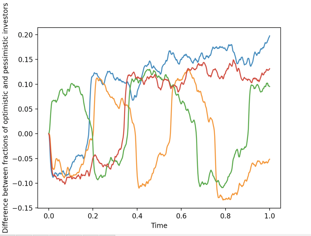


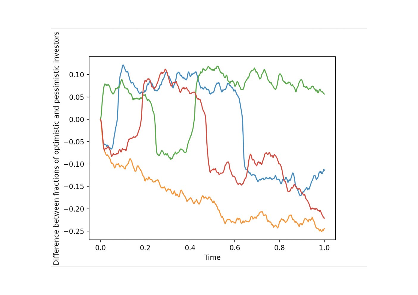
In Figure 2 we plot the function , where is the value for the -th simulated trajectory of the bubble, . The left and right panels show the sample average for and , respectively.
In Figure 3 we plot instead the function above for a sample of trajectories in the case when the values of the fractions of investors are 44 4 We let anyway the bubble start from zero here: one can assume a sudden jump of at initial time, or that before time .. In this case, we see that at the beginning, the bubble blows up on average, because of the actions of the functions and , . However, as the number of pessimistic investors changing their views starts to decrease, the bubble slows down, and then bursts on average because of the action of the mean reverting term in (2.4).
Figure 3 clearly shows that, when the fraction of pessimistic and optimistic investors are different, the bubble is not a martingale under the measure for which we simulate the processes. However, we find a measure under which the expectation of the bubble at time is very close to its value at by tuning the parameters. In particular, this measure is identified by letting the binomial processes driving and increasing with probability and the ones driving and increasing with probability , at the first time step. We see that the average value of is under the first measure and close to under the new measure.


5 Conclusions
We have modeled the formation of asset price bubbles by introducing a random matching mechanism among agents in a discrete time version of the model in [25]. In order to do it, we extend results of [13] to a stochastic setting. In particular, via the introduction of a Markov kernel, we are able to construct the probability space where the asset price process is defined as the product of the space of the random matching and the space of the factors which may influence the transition probabilities. This approach allows to isolate and model the self exciting mechanism governing the blow up of the bubble and the exogenous factors impacting the bursting phase of the bubble. In Section 4.2 we present numerical experiment showing how this approach is able to capture important behavioral features of asset price bubbles.
Appendix A Proof of Proposition 3.12
For every fixed we construct the measure as in the proof of Lemma 7 in [13]. Furthermore, as the construction of the space in Lemma 7 in [13] is independent of the input functions, we can also follow their approach. Then, the definitions of and in Points 1. and 2. in the Proposition allow us to finish the proof. For the readers’s convenience we show the proof in details in the following.
Proof.
Let be the hyperfinite counting probability space with its Loeb space . The proof consists of four steps.
Step 1: For each , and , let
and .
For each , and define a probability on such that
Let be the internal set of all the internal functions from to . For any and , also let be the internal product probability measure on , where is the internal power set of . For each fixed and , the agents in the set are now supposed to be matched with agents in .
Step 2: The issue now is that and might fail to have the same internal cardinality, for , and may fail to have an even internal cardinality, which would allow an internal full matching on . Scope of the second step of the proof is to fix such a problem. For with , let
For any , let be the family of the sets of the form for if is odd, and the set with one element if is even. Set . Define an internal probability measure on with internal power set by letting for .
Let
The probability measure can be trivially extended to the common sample space with its internal power set by letting for .
Given the hyperfinite internal probability space and the internal transition probability , , we can define the internal probability measure on with its internal power set by letting for any and .
Step 3: For any fixed and , we consider the internal partial matchings on that match agents from to . Let , which is the set of initially unmatched agents who remain unmatched. Let denote the set ; then it is clear that . Let . For each , let be the internal set of all the internal full matchings on . Let be the internal counting probability measure on . For with , let be the internal set of all the internal bijections from to . Let be the internal counting probability on . Let be the internal set of all the internal partial matchings from to . Define to be the set of , such that
- 1.
the restriction , where is the set of initially matched agents.
- 2.
for each .
- 3.
The restriction for .
- 4.
For with , .
We now define an internal probability measure on such that
- 1.
for ,
- 2.
For , .
The probability measure can be trivially extended to the sample space .
For any , define an internal probability measure on with the internal power set by letting
| (A.1) |
The construction in (A.1) provides the Markov kernel from to as in Point 2 of the Proposition. From now on, denote for any .
For , let and
Denote the corresponding Loeb probability spaces of the internal probability spaces and by and respectively. Set
Then by construction of , it is clear that . Moreover, is by construction an internal matching and satisfies Point 4. of the proposition.
It is then possible to define as stated in Point 1. and 2. of the proposition and consider the corresponding Loeb probability space, see Point 6. Furthermore, we can extend and to as stated in Point 3. and 5.
Step 4: We now prove Points 5. and 6. of the proposition. Define an internal process from to such that for any we have
Fix from now on and . It is clear that if and , then
which means that
With similar arguments it follows that
Moreover, and are independent random variables on the sample space for any in . The exact law of large numbers as in Lemma 1 in [13] implies that, under the scenario of a current distribution and of a realization , it holds
and
for -almost all and for any , which means that
| (A.2) |
Let be the set of such that (A.2) holds. Then , and hence .
Fix any ; then for some , so .
For any we have
| (A.3) |
which also implies that
For any if and only if ; and if and only if . Hence, for fixed , and for any , we can see that if then
and that if then
For any , that is, for any such that , we have that
It is clear that
which has -measure zero by (A.3). By the fact that , we know that
for -almost all .
Since the Loeb product space is a Fubini extension, the Fubini property implies that for -almost all is equal to for -almost all . Hence satisfies the second part of the Lemma. Let be an -measurable set with such that for any for -almost all . Therefore, by the construction of we know that the collection of random variables is mutually independent in the sense that any finitely many random variables from that collection are mutually independent. This also implies Point 6. of the proposition. ∎
References
- Abreu and Brunnermeier [2003] Dilip Abreu and Markus K. Brunnermeier. Bubbles and crashes. Econometrica, 71(1):173–204, 2003.
- Allen and Gale [2000] F. Allen and D. Gale. Bubbles and crisis. The Economic Journal, 110:236–255, 2000.
- Bayer et al. [2016] Patrick Bayer, Kyle Mangum, and James W. Roberts. Speculative fever: Investor contagion in the housing bubble. Technical report, National Bureau of Economic Research, 2016.
- Becker et al. [2002] Ralf M. Becker, Urs Fischbacher, and Thorsten Hens. Soft landing of a stock market bubble: An experimental study. Zurich IEER Working Paper, 2002.
- Biagini et al. [2014] Francesca Biagini, Hans Föllmer, and Sorin Nedelcu. Shifting martingale measures and the slow birth of a bubble. Finance and Stochastics, 18(2):297–326, 2014.
- Biagini et al. [2018] Francesca Biagini, Andrea Mazzon, and Thilo Meyer-Brandis. Liquidity induced asset bubbles via flows of ELMMs. SIAM Journal on Financial Mathematics, 9(2):800–834, 2018.
- Biagini et al. [2022] Francesca Biagini, Andrea Mazzon, Thilo Meyer-Brandis, and Katharina Oberpriller. Supplement to “liquidity based modeling of asset price bubbles via random matching”. preprint, 2022. URL https://www.fm.mathematik.uni-muenchen.de/personen/professors/francesca_biagini/publications_biagini/index.html.
- Choi and Douady [2011a] Youngna Choi and Raphael Douady. Financial Crisis and Contagion: A Dynamical Systems Approach. 2011a. URL http://ssrn.com/abstract=1733706.
- Choi and Douady [2011b] Youngna Choi and Raphael Douady. Chaos and Bifurcation in 2007-08 Financial Crisis. Management Science, 2011b.
- Cox and Hobson [2005] Alexander M.G. Cox and David G. Hobson. Local martingales, bubbles and option prices. Finance Stochastics, 9(4):477–492, 2005.
- DeLong et al. [1990] J.Bradford DeLong, Andrei Shleifer, Laurence H. Summers, and Robert J. Waldmann. Noise trader risk in financial markets. Journal of Political Economy, 98(4):703?738, 1990.
- Doob [1937] Joseph L. Doob. Stochastic processes depending on continuous parameter. Transactions of the American Mathematical Society, 42, 1937.
- Duffie et al. [2018] Darrell Duffie, Lei Qiao, and Yeneng Sun. Dynamic directed random matching. Journal of Economic Theory, 174:124–183, 2018.
- Duffie et al. [2020] Darrell Duffie, Lei Qiao, and Yeneng Sun. Continuous Time Random Matching. Preprint, 2020. URL https://www.darrellduffie.com/uploads/working/DuffieQiaoSunCTRM_Dec2020.pdf.
- Earl et al. [2007] Peter E. Earl, Ti-Ching Peng, and Jason Potts. Decision-rule cascades and the dynamics of speculative bubbles. Journal of Economic Psychology, 28:351–364, 2007.
- Filardo [2011] Andrew J. Filardo. The impact of the international financial crisis on Asia and the Pacific: Highlighting monetary policy challenges from a negative asset price bubble perspective. BIS Working Paper, 2011.
- Föllmer [2005] Hans Föllmer. Equilibria in financial markets with heterogeneous agents: A probabilistic perspective. Journal of Mathematical Economics, 41(1-2):123–155, 2005.
- Föllmer and Schied [2016] Hans Föllmer and Alexander Schied. Stochastic finance: an introduction in discrete time. De Gruyter, 2016.
- Harrison and Kreps [1978] J. Michael Harrison and David M. Kreps. Speculative investor behavior in a stock market with heterogeneous expectations. The Quarterly Journal of Economics, 92(2):323–336, 1978.
- Jarrow and Protter [2009] Richard Jarrow and Philip Protter. Forward and futures prices with bubbles. International Journal of Theoretical and Applied Finance, 12(7):901–924, 2009.
- Jarrow and Protter [2011] Richard Jarrow and Philip Protter. Foreign currency bubbles. Review of Derivatives Research, 14(1):67–83, 2011.
- Jarrow et al. [2007] Richard Jarrow, Philip Protter, and Kazuhiro Shimbo. Asset price bubbles in complete markets. Advances in Mathematical Finance, In Honor of Dilip B. Madan:105–130, 2007.
- Jarrow et al. [2010] Richard Jarrow, Philip Protter, and Kazuhiro Shimbo. Asset price bubbles in incomplete markets. Mathematical Finance, 20(2):145–185, 2010.
- Jarrow et al. [2011] Richard Jarrow, Younes Kchia, and Philip Protter. How to detect an asset bubble. SIAM Journal on Financial Mathematics, 2:839–865, 2011.
- Jarrow et al. [2012] Robert A. Jarrow, Philip Protter, and Alexandre F. Roch. A Liquidity Based Model for Asset Price Bubbles. Quantitative Finance, 12(1):1339–1349, 2012.
- Kaizoji [2000] Taisei Kaizoji. Speculative bubbles and crashes in stock markets: an interacting-agent model of speculative activity. Phisica A, 287:493–506, 2000.
- Keisler and Sun [2001] Jerome H. Keisler and Yeng Eng Sun. Loeb measures and borel algebras. In Ulrich Berger, Horst Osswald, and Peter Schuster, editors, Reuniting the Antipodes - Constructive and Nonstandard Views of the Continuum, pages 111–117. Kluwer Academic Publishers, Dodrecht, 2001.
- Klenke [2020] Alexander Klenke. Probability Theory A Comprehensive Course. Springer, 2020.
- Loewenstein and Willard [2000] Mark Loewenstein and Gregory A. Willard. Rational equilibrium asset-pricing bubbles in continuous trading models. Journal of Economic Theory, 91(1):17–58, 2000.
- Lux [1995] Thomas Lux. Herd behaviour, bubbles and crashes. The economic journal, 105(431):881–896, 1995.
- Miller [1977] Edward M. Miller. Risk, uncertainty, and divergence of opinion. The Journal of Finance, 32(4):1151–1168, 1977.
- [32] José Scheinkman and Wei Xiong. Technical report.
- Scheinkman and Xiong [2003a] José Scheinkman and Wei Xiong. Overconfidence and speculative bubbles. Journal of political economy, 111(6):1183–1219, 2003a.
- Scheinkman and Xiong [2003b] Jose A. Scheinkman and Wei Xiong. Overconfidence and speculative bubbles. Journal of political Economy, 111(6):1183–1220, 2003b.
- Siegel [2003] Jeremy J. Siegel. What is an asset price bubble? An operational definition. European financial management, 9(1):11–24, 2003.
- Sun [1998a] Yeneng Sun. The theory of hyperfinite processes: the complete removal of individual uncertainty via exact LLN. Journal of Economic Theory, 29, 1998a.
- Sun [1998b] Yeneng Sun. The almost equivalence of pairwise and mutual independence and the duality with exchangeability. Probability Theory and Related Fields, 112(3):425–456, 1998b.
- Sun [2006] Yeneng Sun. The Exact Law of Large Numbers via Fubini extension and characterization of insurable risks. Journal of Economic Theory, 126(1):31–69, 2006.
- Wan [2018] Junmin Wan. Prevention and landing of bubble. International Review of Economics & Finance, 56:190–204, 2018.
- Xiong [2012] Wei Xiong. Bubbles, crises, and heterogeneous beliefs. Technical report, Princeton University, Princeton, NJ, 2012.
- Zhuk [2013] Sergey Zhuk. Speculative bubbles, information flow and real investment. Information Flow and Real Investment, 2013.