A Tree Structure Approach to Reachability Analysis

The development and production of self-driving cars and the deployment of drones in industrial applications are exemplars of society’s ever-increasing fascination of autonomous vehicles. Commensurate to the growing integration of these vehicles in day-to-day life is the concern regarding how safe these unmanned vehicles are. These concerns are particularly prevalent in safety-critical applications such as human-robot interactions, disaster responses, and the use of high-value machinery. In such applications, being able to characterize all possible behaviours of these autonomous vehicles would be a rigorous way to verify their safety. Reachable sets lend themselves well towards this goal. When computed forwards in time, they characterise all possible states that can be reached using a constraint admissible control from some initial set of states. Similarly, when computed backwards in time, they characterise all possible states that are able to reach a terminal set of states using a constraint admissible control.

The computation of reachable sets may be done via the Hamilton-Jacobi-Bellman (HJB) equations, i.e. one of the most powerful formal verification tools for guaranteeing performance and safety properties of systems. This approach is rather general and works for controlled nonlinear systems that involve disturbances or adversarial behaviors, and despite this, characterizes the exact reachable set rather than approximations. However, this method suffers from the curse of dimensionality and it is hard to build numerical methods for high dimensional problems. In the last two decades several contributions on the mitigitation of the curse of dimensionality have been investigated mainly for optimal control problems such as, e.g. model order reduction KVX04; AFV17, tree structure algorithms AFS19; AS20, spectral methods KK18, max-plus algebra M07; M09, Hopf-Lax approaches CDOW19; YD21, neural networks DLM20; DM21, tensor decomposition DKK21; OSS22 and sparse grids method BGGK13.

For the approximation of the reachable sets in MB05, the authors provides a formulation that requires numerically solving a Hamilton-Jacobi partial differential equation. This is a grid-based approach which is typically limited to systems of no more than 4 states on standard computers. Therefore, the study of higher dimensional problems remains an open research area. Under certain assumption on the system, one could decompose it appropriately, and obtain efficient algorithms for computing reachable sets, see e.g. CHVBT18. Other approaches have been studied in AK13 where reachable sets for nonlinear systems are computed via results on reachability for uncertain linear system. Linearisation error is explicitly accounted for in AK13 using an iterative algorithm to bound this error in an over-approximative manner. Similarly, in YA21, uncertain linear systems are considered with a focus on producing zonotopic under-approximations of reachable sets. In their work, the representational complexity of the reachable sets grows as the algorithm iterates in time, thus motivating the use of a ‘pruning’ step, which reduces the order of the zonotopic sets.

In this paper, we present an algorithm based on a tree structure to approximate the HJB equation for backwards reachable sets. The idea of the algorithm is based on the paper AFS19 and approximates the value function using the Dynamic Programming Principle (DPP) on an unstructured mesh for optimal control problems. The idea of our proposed algorithm is as follows.

We start from a discretization of the terminal set and compute the value function on those points. Then, we neglect the interior points, say those nodes for which the value function is strictly negative. This is a pruning strategy that aims to mitigate the exponential increase in the cardinality of the tree. We then evolve these nodes backwards in time, making use of a result provided in Section 4, where the forward controlled dynamical system is equivalent, up to minor changes in the problem, to the backward system. This is the main difference with respect to the method in AFS19. We are able, in this work, to compute the tree backwards in time and to prune the tree using the information from the value function. Our pruning is based on geometric considerations where the interior of the reachable set is pruned. This comes from the observation, which is demonstrated in this work, that the boundary of the reachable set at a particular time cannot evolve from the interior of the reachable set at a prior time. Thus, it is wasteful to propagate the tree structure of AFS19 for nodes that lie interior to the reachable set. When the value function is convex, interior nodes can be easily identified using off-the-shelf algorithms for computing convex hulls.

The outline of the paper is the following. In Section 2 we present the control problem setup and in Section 3 we provide the relevant background for the characterization of the backwards reachable set. In Section 4 we show the equivalence between backwards and forwards reachable sets. Our algorithm is introduced and discussed in Section 5. Numerical examples are then shown in Section 6. Finally, conclusions and future works are discussed in Section 7.

• •

  Let $\mathbb{I}_{n}$ denote an $n$-by-$n$ identity matrix.

• •

  Let $\langle\cdot,\cdot\rangle$ denote the Euclidean inner product.

• •

  Let $\lVert w\rVert$ denote any norm of a vector $w$.

• •

  Let $int\left(\mathcal{A}\right),cl\left(\mathcal{A}\right)$, and $\partial\mathcal{A}$ denote the interior, closure, and boundary of a set $\mathcal{A}$, respectively.

• •

  Let $\mathcal{C}^{k}(\Omega;\,\mathbb{R})$ denote the space of $k$-times continuously differentiable functions from $\Omega$ to $\mathbb{R}$ with $\mathcal{C}\doteq\mathcal{C}^{0}$.

• •

  Let $\mathbb{B}_{R}(x_{0})\doteq\{x\in\mathbb{R}^{n}\,|\,\lVert x-x_{0}\rVert\leq R\}$ denote a ball of radius $R\geq 0$ with centre $x_{0}\in\mathbb{R}^{n}$.

• •

  An ellipsoidal set with centre $q$ and shape $Q$ is defined as

  $$\mathcal{E}(q,Q)\doteq\left\{x\in\mathbb{R}^{n}\,|\,(x-q)^{T}Q^{-1}(x-q)\leq 1\right\},$$

  (1)

  where $q\in\mathbb{R}^{n}$ and $Q\in\mathbb{R}^{n\times n}$ is a symmetric, positive definite matrix. The axes of $\mathcal{E}(q,Q)$ are aligned with the eigenvectors of $Q$ with lengths along these axes being equal to the square root of the corresponding eigenvalues.

• •

  Let $\text{conv}\left(\mathcal{A}\right)$ denote the convex hull of a finite set of points $\mathcal{A}=\{a_{i}\}_{i\in\{1,\cdots,n_{p}\}}$, defined by

  $$\text{conv}\left(\mathcal{A}\right)=\left\{\sum^{n_{p}}_{i=1}\lambda_{i}a_{i}\,\Bigg|\,\lambda_{i}\geq 0\text{ for all }i\in\{1,\cdots,n_{p}\}\text{ and }\sum^{n_{p}}_{i=1}\lambda_{i}=1\right\}.$$

  (2)

In this section we begin with a system description and review relevant background relating to optimal control. Consider the continuous-time nonlinear system described by

where $T\geq 0$, $x(t)\in\mathbb{R}^{n}$ is the state and $u(t)\in\mathbb{U}$ is the input at time $t$, with $\mathbb{U}\subset\mathbb{R}^{m}$ being compact. The input is selected such that $u\in\mathcal{U}$, where

The following flow field conditions are assumed throughout. {assumption} The function $f:\mathbb{R}^{n}\times\mathbb{U}\rightarrow\mathbb{R}^{n}$ satisfies

1. i)

   $f\in\mathcal{C}\left(\mathbb{R}^{n}\times\mathbb{U}\,;\mathbb{R}^{n}\right)$; and

2. ii)

   $f$ is locally Lipschitz continuous in $x$, uniformly in $u$, i.e. for any $R>0$, there exists a Lipschitz constant $C^{f}_{R}>0$ such that $\lVert f(x,u)-f(y,u)\rVert\leq C^{f}_{R}\lVert x-y\rVert,\;\;\forall(x,y,u)\in\mathbb{B}_{R}(0)\times\mathbb{B}_{R}(0)\times\mathbb{U}$.

Under Assumption 2, the system described by (3) admits a unique and continuous solution for any initial condition $x(0)=x_{0}$ and fixed control $u(\cdot)\in\mathcal{U}$. We denote these solutions at time $0\leq t\leq T$ by $\varphi(t;0,x_{0},u(\cdot))$.

Attach to (3) the value function $V:[0,T]\times\mathbb{R}^{n}$ corresponding to the optimal control problem

where the running cost $h:\mathbb{R}^{n}\times\mathbb{U}\rightarrow\mathbb{R}$ and the terminal state cost $g:\mathbb{R}^{n}\rightarrow\mathbb{R}$ satisfy the assumptions below. {assumption} The functions $h:\mathbb{R}^{n}\times\mathbb{U}\rightarrow\mathbb{R}$ and $g:\mathbb{R}^{n}\rightarrow\mathbb{R}$ satisfy

1. i)

   $h\in\mathcal{C}\left(\mathbb{R}^{n}\times\mathbb{U};\,\mathbb{R}\right)$ and $g\in\mathcal{C}\left(\mathbb{R}^{n};\,\mathbb{R}\right)$; and

2. ii)

   $h$ and $g$ are locally Lipschitz continuous in $x$ (uniformly in $u$ for $h$), i.e. for any $R>0$, there exists a Lipschitz constant $C^{h}_{R}>0$ such that $|h(x,u)-h(y,u)|\leq C^{h}_{R}\lVert x-y\rVert,\;\;\forall(x,y,u)\in\mathbb{B}_{R}(0)\times\mathbb{B}_{R}(0)\times\mathbb{U}$ and there exists a $C^{g}_{R}>0$ such that $|g(x)-g(y)|\leq C^{g}_{R}\lVert x-y\rVert,\;\forall(x,y)\in\mathbb{B}_{R}(0)\times\mathbb{B}_{R}(0)$.

The value function defined by (5) satisfies the Dynamic Programming Principle (see e.g. BCD97), which is presented below.

The value function can be characterized via the viscosity solution of a HJB equation. A detailed discussion on viscosity solutions can be found in crandall1983viscosity.

Let us now consider a special case of the optimal control problem in (5), which can be used to characterize a backwards reachable set. This set characterizes all states $x\in\mathbb{R}^{n}$ for which there exists an admissible control $u(\cdot)\in\mathcal{U}$ leading to some terminal set of states

in time $T\geq 0$, where $g:\mathbb{R}^{n}\rightarrow\mathbb{R}$ is a bounded and locally Lipschitz continuous function. The backwards reachable set is more precisely defined below.

The backwards reachable set can be characterized via the viscosity solution of the HJB equation given in (7)–(8), which is described in the following theorem (see e.g. BCD97).

Next, we will demonstrate that the boundary of the backwards reachable set $\mathcal{G}(T)$ can only reach the boundary of the terminal set $\mathcal{X}_{T}$. This result will motivate the use of a geometric pruning criterion that will be introduced in our proposed algorithm for computing $\mathcal{G}(T)$.

An analogous set to the backwards reachable set is the forwards reachable set, which characterizes all states that can be reached from some initial set of states under the influence of an admissible control. We will verify that the forwards reachable set of a time-reversed system is exactly the backwards reachable set of (3). This will prove to be convenient for us as the algorithm in Section 5 is more intuitively described when considering a forwards reachability problem. The aforementioned time-reversed system is described by

where $T\geq 0$, $f:\mathbb{R}^{n}\times\mathbb{U}\rightarrow\mathbb{R}^{n}$ satisfies Assumption 2, and $u(\cdot)\in\mathcal{U}$. When referring to the forwards reachable set, we will use $\mathcal{X}_{0}$ defined identically to $\mathcal{X}_{T}$ in (9) to describe the initial set of states. The forwards reachable set for (15) is now precisely defined below.

To demonstrate that $\mathcal{F}_{-}(T)$ is exactly the backwards reachable set $\mathcal{G}(T)$, we formally verify a standard result relating solutions of (3) to (15). In particular, we wish to show that an initial state $x$ that evolves under a control $u(\cdot)$ for (3) can be recovered by setting the terminal state of (3) as the initial state for (15) and applying a time-reversed control $u_{-}(\cdot)$. It follows naturally that the other direction would hold as well. This is more precisely described below.

Likewise with the characterization of the backwards reachable set in Theorem 13, the forwards reachable set $\mathcal{F}_{-}(T)$ for (15) can be also be characterized via the solution of a corresponding HJB PDE.

In this section we provide the description of our new algorithm to approximate solutions of (7) with zero running cost, i.e. $h=0$. Our algorithm is based on a tree structure as proposed in AFS19 that is adapted to our problem for computing the backwards reachable set as defined in (10). This tree structure is depicted in Figure 1. In AFS19, the value function is computed by first constructing a tree, which represents a discretization in time and space of the forwards reachable set from a known initial state denoted by $x^{0}_{1}$ in the diagram. Using the Dynamic Programming Principle (DPP) stated in Theorem 6, the value function is then computed backwards in time starting from the nodes in the tree corresponding to some terminal time $t=T$. However, when it comes to computing the backwards reachable set, we want to compute the set of all initial states such that a known terminal set $\mathcal{X}_{T}$ can be reached. Thus, a key difference between our approach and the algorithm proposed in AFS19 is that we build the tree backwards in time starting from time $T$ at the terminal set. We now move to describing how the algorithm of AFS19 could be adjusted to compute the backwards reachable set and state its connection to the value function in (5). A geometric condition for pruning is then introduced to reduce the computational expense.

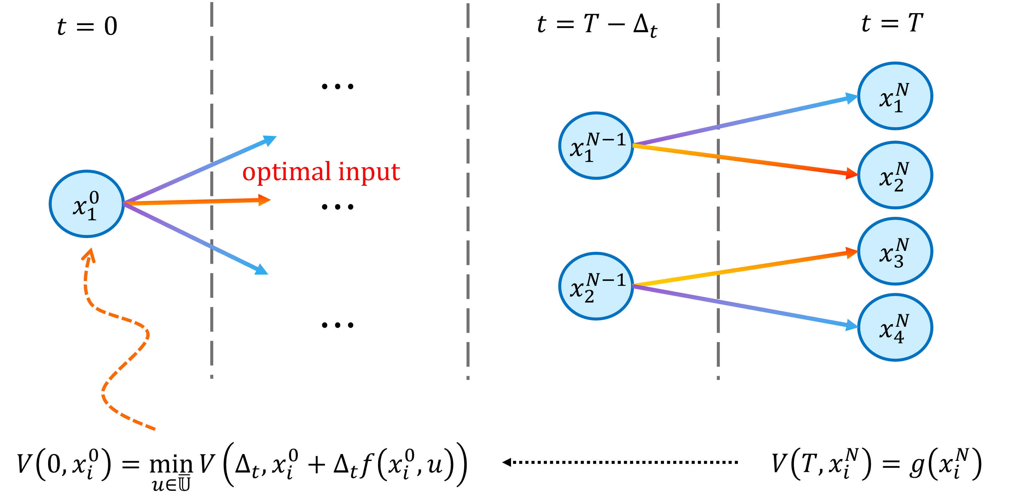
To begin, the control set $\mathbb{U}$ is discretized into a finite set $\bar{\mathbb{U}}\doteq\{u_{1},\ldots,u_{n_{u}}\}\subset\mathbb{U}$. Let $\Delta_{t}$ denote the time discretization interval with $t_{k}\doteq T-k\Delta_{t}$ being the $k$-th time point for a total of $N\doteq\lceil\textstyle{\frac{T}{\Delta_{t}}}\rceil$ time points. We define the $k$-th tree level $\mathcal{T}^{k}$ as the set of nodes generated at time $t_{k}$, which has a cardinality denoted by $n_{k}$. Additionally, we use $x^{k}_{i}$ to denote the $i$-th node of the $k$-th tree level.

Then, we start to compute the nodes of our tree. The initial (zeroth) level contains nodes given by a discretization of the terminal set $\mathcal{X}_{T}$. Let $\{x^{0}_{i}\}_{i\in\{1,\ldots,n_{0}\}}$ be a finite set of points in $\mathcal{X}_{T}$. For these points, we can directly compute the value function as follows:

which is given by the terminal condition of (11) at time $T$. Equivalently, we can consider this step as initialising the value function $w$ in (21) for the forwards reachable set of the time-reversed system in (15).

We continue generating the nodes of the tree for level $1$ corresponding to the time $t_{1}=T-\Delta_{t}$. The set of nodes $\mathcal{T}^{1}\doteq\{x^{1}_{i}\}_{i\in\{1,\ldots,n_{1}\}}$ will be computed from the time-reversed ODE (15). Although other discretizations are possible, an Euler discretization has been chosen here leading to:

Once the nodes in $\mathcal{T}^{1}$ are generated we approximate the value function at time $T-\Delta_{t}$ using a one-step discretisation of the DPP (rewritten from (6)) using the discretized input set $\bar{U}$:

The DPP in (29) approximates the value function for a point $x^{1}_{i}$ at time $T-\Delta_{t}$ via a minimization of the value function at time $T$ across all points that can be reached by $x^{1}_{i}$ forwards in time. However, the value function at time $T$ is only computed in (27) on the finite set of points $\mathcal{T}^{0}=\left\{x^{0}_{i}\right\}_{i\in\{1,\ldots,n_{0}\}}$, which may not contain the point $x^{1}_{i}+\Delta_{t}f(x^{1}_{i},u_{j})$. In general, (29) may require an interpolation of the value function.

In order to compute an approximation of the value function using pre-computed values of nodes on previous tree levels, we can instead perform the minimization in (29) over all nodes in $\mathcal{T}^{0}$ that can be reached by $x^{1}_{i}$. To be more precise, we consider an Euler discretisation of the forward system (3):

where $x[n]\approx x(T-t_{n}),$ $u[n]\approx u(T-t_{n})\in\mathbb{U},\;\forall n\in\{0,1,\ldots\}$. The set of points that can be reached in a single time-step $\Delta_{t}$ is defined precisely below.

From this, we construct a general iteration step for generating nodes on all tree levels $k\in\{1,\ldots,n_{k}\}$, as well as approximating the value function at these nodes:

In (32), we generate nodes contained in the forwards reachable set of the time-reversed system in (15) starting from an initial set $\mathcal{X}_{0}=\mathcal{X}_{T}$. From Theorem 20, this gives us the backwards reachable set of (3). The value function is then approximated via a minimization over a subset of nodes in the previous tree level. Unlike in Figure 1, the entire tree does not need to be generated a priori. Algorithm 1 summarises the procedure outlined above.

As the number of nodes grows by a factor of $n_{u}$ in each tree level $k$ of Algorithm 1, a pruning strategy becomes necessary to mitigate the exponential increase in the cardinality of the tree. In AFS19, a pruning strategy based on the distance of the nodes on the same level of the tree was implemented. This turned out to be efficient due to the fact that the value function is a Lipschitz continuous function. Here, in our problem, we offer an alternative pruning criterion based on storing only the nodes that lie along the boundary of the reachable set. In Lemma 1, it was shown that the boundary of the backwards reachable set cannot come from the interior of the terminal set $\mathcal{X}_{T}$. This applies in a recursive manner, meaning, the boundary of the backwards reachable set at time $t$ cannot come from the interior of the set at a time $\tau>t$. Thus, propagating the tree from nodes that lie in the interior of the backwards reachable set seems to be a wasted expense.

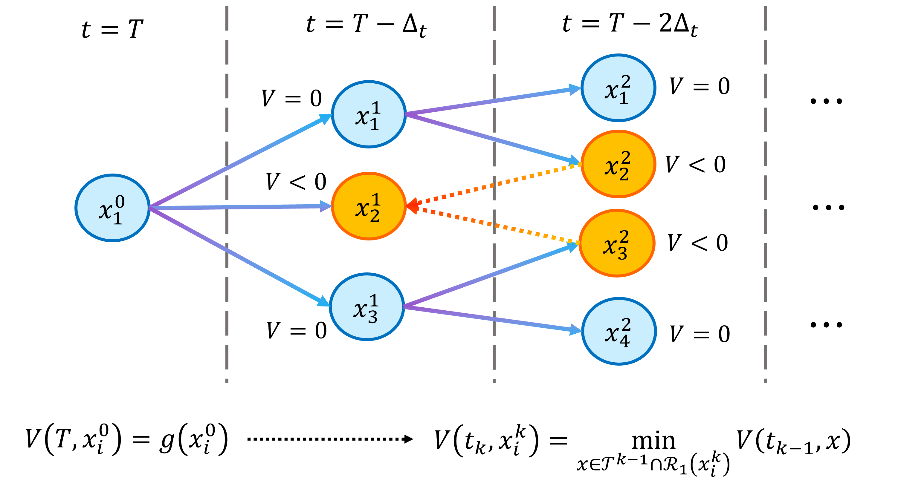
Interior nodes can be identified by points for which $V(t,x)<0$, and are candidates for pruning. Algorithm 1 could potentially be modified in Steps 2 to 5 with a pruning step that removes nodes in $\mathcal{T}^{k}$ if $V(t_{k},x^{k}_{i_{j}})<-\epsilon$ for some chosen tolerance $\epsilon>0$. However, removing all such nodes may be problematic as (33) minimizes over all nodes in the previous level $k-1$. If none of the nodes in the previous level have a value less than $-\epsilon$, then it is not possible for any node on level $k$ to have a value less than $-\epsilon$ and hence interior nodes can no longer be identified. This issue is highlighted in Figure 2. If nodes $x^{2}_{2}$ and $x^{2}_{3}$ can reach node $x^{1}_{2}$ using an input $u\in\mathbb{U}$ and $V(T-\Delta_{t},x^{1}_{2})<0$, then it must also be the case that the value at these nodes is also strictly negative, and are hence interior nodes. However, if $x^{1}_{2}$ is pruned from the previous level, then $x^{2}_{2}$ and $x^{2}_{3}$ can no longer be identified as interior nodes. In general, some interior nodes may need to be stored so that nodes on further tree levels can be identified as being interior. These nodes can then be stored more sparsely by removing some of its members without impacting knowledge of the boundary of the reachable set.

There is, however, a case where interior nodes can be identified without needing to store interior nodes in previous tree levels. In particular, a geometric condition for identifying interior nodes can be used. To this extent, first consider the short result below.

It follows from Lemma 35 that for convex value functions, points that lie interior to the convex hull of the nodes on any given tree level $k$ must also be interior to the backwards reachable set $\mathcal{G}(t_{k})$ (ignoring integration errors of (32)). This implicitly identifies nodes for which $V<0$.

A modification to Algorithm 1 is presented in Algorithm 2 where assumptions on convexity are used to avoid explicit computation of the value function for identifying interior points. Here $\tilde{\mathcal{T}}^{k}$ denotes the tree at level $k$ containing a set of nodes $\{\tilde{x}^{k}_{i}\}_{i\in\{1,\ldots,\tilde{n}_{k}\}}$ prior to any pruning. If a node in $\tilde{\mathcal{T}}^{k}$ lies interior to the convex hull of $\tilde{\mathcal{T}}^{k}$, it is not added to the tree level $\mathcal{T}^{k}$, and is thus not propagated in the overall tree structure.

References

- (1) K. Kunisch, S. Volkwein, L. Xie, HJB-POD-based feedback design for the optimal control of evolution problems, SIAM Journal on Applied Dynamical Systems 3 (4) (2004) 701–722.
- (2) A. Alla, M. Falcone, S. Volkwein, Error analysis for POD approximations of infinite horizon problems via the dynamic programming approach, SIAM Journal on Control and Optimization 55 (5) (2017) 3091–3115.
- (3) A. Alla, M. Falcone, L. Saluzzi, An efficient DP algorithm on a tree-structure for finite horizon optimal control problems, SIAM Journal on Scientific Computing 41 (4) (2019) A2384–A2406.
- (4) A. Alla, L. Saluzzi, A HJB-POD approach for the control of nonlinear PDEs on a tree structure, Applied Numerical Mathematics 155 (2020) 192–207, Structural Dynamical Systems: Computational Aspects held in Monopoli (Italy) on June 12-15, 2018. doi:https://doi.org/10.1016/j.apnum.2019.11.023.
- (5) D. Kalise, K. Kunisch, Polynomial Approximation of High-Dimensional Hamilton–Jacobi–Bellman Equations and Applications to Feedback Control of Semilinear Parabolic PDEs, SIAM Journal on Scientific Computing 40 (2) (2018) A629–A652.
- (6) W. M. McEneaney, A curse-of-dimensionality-free numerical method for solution of certain HJB PDEs, SIAM journal on Control and Optimization 46 (4) (2007) 1239–1276.
- (7) W. M. McEneaney, Convergence rate for a curse-of-dimensionality-free method for Hamilton–Jacobi–Bellman PDEs represented as maxima of quadratic forms, SIAM Journal on Control and Optimization 48 (4) (2009) 2651–2685.
- (8) Y. T. Chow, J. Darbon, S. Osher, W. Yin, Algorithm for overcoming the curse of dimensionality for state-dependent Hamilton-Jacobi equations, Journal of Computational Physics 387 (2019) 376–409.
- (9) I. Yegorov, P. M. Dower, Perspectives on characteristics based curse-of-dimensionality-free numerical approaches for solving Hamilton-Jacobi equations, Applied Mathematics & Optimization 83 (1) (2021) 1–49.
- (10) J. Darbon, G. P. Langlois, T. Meng, Overcoming the curse of dimensionality for some Hamilton–Jacobi partial differential equations via neural network architectures, Research in the Mathematical Sciences 7 (3) (2020) 1–50.
- (11) J. Darbon, T. Meng, On some neural network architectures that can represent viscosity solutions of certain high dimensional Hamilton–Jacobi partial differential equations, Journal of Computational Physics 425 (2021) 109907.
- (12) S. Dolgov, D. Kalise, K. K. Kunisch, Tensor Decomposition Methods for High-dimensional Hamilton–Jacobi–Bellman Equations, SIAM Journal on Scientific Computing 43 (3) (2021) A1625–A1650.
- (13)
M. Oster, L. Sallandt, R. Schneider,
Approximating optimal feedback
controllers of finite horizon control problems using hierarchical tensor
formats, SIAM Journal on Scientific Computing 44 (3) (2022) B746–B770.
arXiv:https://doi.org/10.1137/21M1412190, doi:10.1137/21M1412190.
URL https://doi.org/10.1137/21M1412190 - (14) O. Bokanowski, J. Garcke, M. Griebel, I. Klompmaker, An adaptive sparse grid semi-Lagrangian scheme for first order Hamilton-Jacobi Bellman equations, Journal of Scientific Computing 55 (3) (2013) 575–605.
- (15) B. A. Mitchell, I.M., C. Tomlin, A time-dependent hamilton-jacobi formulation of reach- able sets for continuous dynamic games., IEEE Trans. on Automatic Control, 50 (7) (2005) 947–957.
- (16) M. Chen, S. Herbert, M. Vashishtha, S. Bansal, C. Tomlin, Decomposition of reachable sets and tubes for a class of nonlinear systems., IEEE Trans. on Automatic Control, 63 (11) (2018) 3675–3688.
- (17) M. Althoff, B. Krogh, Reachability analysis of nonlinear differential-algebraic systems., IEEE Trans. on Automatic Control 59 (2) (2013) 371–383.
- (18) L. Yang, N. Ozay, Scalable zonotopic under- approximation of backward reachable sets for uncertain linear systems., IEEE Control Systems Letters 6 (2021) 1555– 1560.
- (19) M. Bardi, I. Capuzzo-Dolcetta, Optimal Control and Viscosity Solutions of Hamilton-Jacobi-Bellman Equations, Birkhäuser, Basel, 1997.
- (20) M. G. Crandall, P.-L. Lions, Viscosity solutions of Hamilton-Jacobi equations, Transactions of the American mathematical society 277 (1) (1983) 1–42.
- (21) P. Cannarsa, C. Sinestrari, Semiconcave functions, Hamilton-Jacobi equations, and optimal control, Vol. 58, Springer Science & Business Media, 2004.
- (22) F. Borrelli, A. Bemporad, M. Morari, Predictive control for linear and hybrid systems, Cambridge University Press, 2017.
- (23) R. T. Rockafellar, Convex analysis, Vol. 18, Princeton university press, 1970.
- (24)
I. M. Mitchell, A
toolbox of level set methods.
URL https://www.cs.ubc.ca/$\sim$mitchell/ToolboxLS/ - (25) C. B. Barber, D. P. Dobkin, H. Huhdanpaa, The quickhull algorithm for convex hulls, ACM Transactions on Mathematical Software (TOMS) 22 (4) (1996) 469–483.