Fast Community Detection in Dynamic and Heterogeneous Networks
Abstract
Dynamic heterogeneous networks describe the temporal evolution of interactions among nodes and edges of different types. While there is a rich literature on finding communities in dynamic networks, the application of these methods to dynamic heterogeneous networks can be inappropriate, due to the involvement of different types of nodes and edges and the need to treat them differently.In this paper, we propose a statistical framework for detecting common communities in dynamic and heterogeneous networks. Under this framework, we develop a fast community detection method called DHNet that can efficiently estimate the community label as well as the number of communities. An attractive feature of DHNet is that it does not require the number of communities to be known a priori, a common assumption in community detection methods. While DHNet does not require any parametric assumptions on the underlying network model, we show that the identified label is consistent under a time-varying heterogeneous stochastic block model with a temporal correlation structure and edge sparsity. We further illustrate the utility of DHNet through simulations and an application to review data from Yelp, where DHNet shows improvements both in terms of accuracy and interpretability over existing solutions.
Keywords: dynamic heterogeneous network, modularity, community detection, null model, consistency, Yelp reviews.
1 Introduction
One of the fundamental problems in network data analysis is community detection that aims to divide the network into non-overlapping groups of nodes such that nodes within the same community are densely connected and nodes from different communities are relatively sparsely connected. Community detection can provide valuable insights on the organization of a network and greatly facilitate the analysis of network characteristics. As such, community detection methods have been applied to numerous scientific fields such as social science (Moody and White 2003), biology (Sørlie et al. 2001) and business (Linden et al. 2003). Over the past few decades, the problem of community detection has been approached from methodological, algorithmic and theoretical perspectives with substantial developments. We refer to Fortunato 2010 and Abbe 2017 for comprehensive reviews on this topic.
While the majority of existing community detection methods are developed for a homogeneous network or a dynamic network, networks that are dynamic and heterogeneous are fast emerging in recent years. For example, in a dynamic healthcare network, nodes can be patients, diseases, doctors and hospitals and edges can be in the type of patient-disease (patient treated for disease) and patient-doctor (patient treated by doctor) and doctor-hospital (doctor works at hospital). These edges are expected to evolve with time as patients may develop new diseases that are treated by different doctors at possibly different hospitals. Figure 1 provides an illustration of a dynamic heterogeneous Yelp review network, which is analyzed in Section 6. In this figure, there are three types of nodes including users, businesses and categories and three types of edges including user-user (user is friend with user), user-business (business is reviewed by user) and business-category (business is labeled with category). As users review different businesses over time, this network is both heterogeneous and dynamic.

Due to the rich information embedded in a dynamic heterogeneous network, many methods have been developed recently for its analysis, such as network embedding (Wang et al. 2022; Zhang et al. 2022), representation learning (Yin et al. 2019) and link prediction (Xue et al. 2020; Jiang et al. 2021). However, community detection in dynamic heterogeneous networks is less studied. One relevant work is Sun et al. 2010, which provides a mixture model-based generative model for estimating the community structure, which is assumed to be time-varying. Other works on this topic include Sengupta and Chen 2015 and Zhang and Cao 2017, though they only focus on a single heterogeneous network.
In our work, we focus on detecting common communities in a dynamic heterogeneous network, that is, the community assignment does not vary with time but the interactions within and between communities do. Finding common communities are useful in many applications. For example, in genetic studies and brain connectivity studies, the common communities represent functional groups of genes or brain regions that are coordinated in biological processes, and identifying them is of keen scientific interests (Zhang and Cao 2017; Zhang et al. 2020). In the Yelp review network, it is plausible that businesses, categories and the majority of users have a common community structure over time, as the service offered by a business and the interests of users (e.g., pets, parks, fine dining) are often stable over a period of time. One notable advantage of considering a common community structure is that the networks observed at different time points are allowed to be highly sparse if , the number of time points, increases. For example, we show in Theorem 1 that consistent community detection is achievable as long as , where is the average degree, while the single network case requires to achieve community detection consistency. Moreover, our approach allows the community strength to be highly variable over time. For example, a community needs to be active for only a very short period of time for it to be consistently identified; see more discussions after Theorem 1.
In this paper, we propose a statistical framework for modularity-based common community detection in the dynamic heterogeneous network, where no parametric assumptions are made on the model underlying the observed networks. Under this framework, we develop a fast community detection method called DHNet that can efficiently estimate the community label as well as the number of communities. An attractive feature of DHNet is that it does not require the number of communities to be known a priori, a common assumption in community detection methods. Although DHNet does not rely on parametric assumptions on the underlying network model, we propose a new dynamic heterogeneous stochastic block model with a temporal correlation structure and edge sparsity, and show that DHNet can consistently estimate the community label under this model. This provides theoretical justifications of the proposed method and also sheds lights on how different network properties (e.g., sparsity, size, community strength) affect its performance. The consistency property of our method when applied to dynamic bi-partite or multi-partite networks follows as special cases.
The remainder of the article is organized as follows. Section 2 describes a community detection framework and proposes a modularity function for finding common communities in a dynamic heterogeneous network. Section 3 describes a fast community detection method called DHNet that can efficiently estimate the community label as well as the number of communities. Section 4 shows the consistency property of DHNet under a dynamic heterogeneous stochastic block model. Section 5 demonstrates the efficacy of DHNet through simulation studies and Section 6 applies the proposed method to review data from Yelp. The paper is concluded with a short discussion section.
2 Community Detection with Modularity
2.1 Notation
We write for an integer . To ease notation, we start the introduction with a single heterogeneous networks with types of nodes. Let be the set containing the -th type of nodes for , where is the number of -th type nodes. Denote the heterogeneous network as , where set contains edges between nodes of the same type and set contains edges between nodes of different types. When , forms a multi-partite network, i.e., edges are only established between different types of nodes. Let denote the homogeneous network formed within node set with an adjacency matrix , and denote the bi-partite network formed between node sets and with an bi-adjacency matrix , . See Figure 2 for an example of a heterogeneous network with .
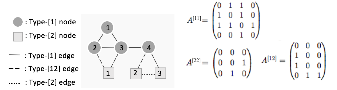
Consider a dynamic heterogeneous network with types of nodes, where is a heterogeneous network at time defined as above. The network at time can be uniquely represented by its adjacency matrix defined as
where is defined as in Figure 2. Define , where is the number of links incident to from at time , and , where is the number of links incident to from at time . Write the number of edges in as for .
2.2 Modularity function
The modularity function measures the strength of division of a network into communities, and the maximum modularity function value is a metric frequently used for quantifying the strength of community structure within a network (Fortunato 2010). The function was first defined in Newman and Girvan 2004 for a simple network with nodes, edges, adjacency matrix and a community assignment , where , as
| (1) |
where is the indicator function. In (1), the expectation is calculated under a null model for random networks with no community structure. The most common choice for the null model is the Chung-Lu model (Newman and Girvan 2004; Newman 2006). In a Chung-Lu model (Chung et al. 2006), given the expected degrees for the nodes, the probability of having an edge between nodes and depends only on the their expected degrees. As noted by Newman 2006, the Chung–Lu model is the only random graph model where the probability of having an edge between nodes and is the product of separate functions of the expected degrees of nodes and , written as , where the functions must be the same since the adjacency matrix is symmetric. Under the Chung–Lu model, it has been shown that every network in the null space occurs with the same probability and there is no preference for any particular graph configuration (Zhang and Chen 2017), which makes the model a desirable choice as the null. It is seen that the modularity function in (1) measures the difference between the observed number of intra-community edges and the expected number of intra-community edges under the null with no community structure. Correspondingly, the community label of a network is identified by maximizing the modularity function with respect to .
To define the modularity function in a dynamic heterogeneous network, we first describe the corresponding null model that characterizes a dynamic heterogeneous network with no community structure. Consider the heterogeneous network at time , with degree sequence . We define a heterogeneous Chung-Lu model as the null. Specifically, under the null, we assume that a heterogeneous network at time is generated with
| (2) |
where all edges in are independent. Under (2), it is easy to show that the expected degree sequence under the null is the same as the observed degree sequence . Following the same argument as in Zhang and Chen 2017, it can be shown that under (2), every heterogeneous network in the null space occurs with the same probability.
Next, we move to define the modularity matrix. At time and given , we write the modularity matrix as
where . The modularity matrix measures the distance between the observed network and the expected network under the null model at time . Given the dynamic heterogeneous networks , the integrated modularity matrix is defined as
. The integrated modularity matrix measures the distance between the observed network and the expected network under the null model over all .
We are now ready to define the modularity function. Write the community assignment label as with , the modularity function of the dynamic heterogeneous network is defined as
| (3) |
From the above definitions, it can be shown that . This modularity function measures the overall difference between the observed number of intra-community edges and the expected number of intra-community edges under the null model. When approaches 1, the observed number of intra-community edges is greater than the expected values, which indicates a strong community structure. In contrast, when approaches 0, the observed number of intra-community edges is close to the expected values under the null, which indicates no or weak community structure.
In practice, the networks are often only observed on a number of time points , where is the total number of observations or snapshots. In this case, we can define
| (4) |
where , , and write the modularity function as
where . The above modularity function can be considered as an averaged version of the modularity in each graph , .
3 Modularity maximization
We aim to find the community assignment that maximizes the modularity function (3), that is,
| (5) |
Finding the exact maximizer of (3) is challenging due to the combinatorial nature of the problem and the fact that the number of communities is generally unknown. Brandes et al. 2008 showed that finding the partition that maximizes the modularity function for a simple graph is NP-hard. There are a number of existing heuristic algorithmic solutions to maximizing the modularity function, some of which are fast and hence feasible for very large networks (Clauset et al. 2004; Wakita and Tsurumi 2007; Blondel et al. 2008), while some others could be more precise though restricted to graphs of moderate sizes (Guimera et al. 2004; Massen and Doye 2005).
In our approach, we adopt a fast Louvain-type maximization method. The Louvain method was first proposed by Blondel et al. 2008 for modularity maximization in simple graphs. In the Louvain method, small communities are first identified by optimizing the modularity function locally on all nodes. Then each small community is grouped into one “meta” node and the first step is repeated. The Louvain method is fast to compute and enjoys a good empirical performance. It has been successful applied to network analyses from various scientific fields, permitting up to 100 million nodes and billions of edges. Notably, the modularity maximum found by the Louvain method often compares favorably with those found by alternative methods such as Clauset et al. 2004 and Wakita and Tsurumi 2007; see Fortunato 2010.
Motivated by the Louvian algorithm, we propose a dynamic heterogeneous network modularity maximization algorithm, referred to DHNet. To do so, we first define a unit, which is set of nodes with at most one from each node type. For example, a unit may contain one node of any type or nodes of different types. A unit serves as the building block of a community in a heterogeneous network. Next, given a heterogeneous modularity matrix as in (4), we define a modularity network, which is a network of nodes and the edge between nodes is . From (3) and (5), it is easy to see that our optimization task is to find a partition of the modularity network such that the within-community sum of edges from is maximized.
The algorithm DHNet starts with assigning each node to its own unit and then each unit to its own community, leading to communities at the start of the algorithm with each community containing only one node (or unit). The optimization procedure is then carried out in two phases that are repeated iteratively. In the first phase and for each unit , DHNet removes this unit from its current community and assigns it to its neighboring community (communities to which unit is linked to), such that it leads to the largest increase of the modularity in (3). If no move increases the modularity, then unit remains in its current community. In the second phase, the algorithm merges nodes of the same type in each community, such that each community contains at most one node from each node type, and builds a new modularity network. In the new modularity network, the units are communities from the first phase and the edge between two nodes are given by summing the edge weights connecting two corresponding sets of nodes from the first phase. These steps are repeated iteratively until the modularity value no longer increases. The algorithm can be summarized as Algorithm 1.
Input: Dynamic heterogeneous networks ,…, .

Figure 3 shows an example of applying DHNet to a dynamic heterogeneous network with two types of nodes. First, Step 1 calculates the modularity matrix from heterogeneous networks ,…, as in (4) and Step 2 assigns each node to its own unit and assign each unit to its own community. Then Step 3 is implemented once and the algorithm reaches convergence. Specifically, in Figure 3 and after Steps 3.1-3.2, nodes , and are placed into three communities, colored black, red and blue, respectively. Step 3.3 then produces a new modularity network with 6 nodes and 3 units. The first unit has nodes and 7, where nodes and are merged as they are of the same type. Similarly, the second unit has and 8 and the third unit has and 9. After this step, merging any of the three units cannot further increase the modularity and thus DHNet returns three communities with nodes , and , respectively.
Remark 1 (initialization). In Step 3.1, if there are multiple communities that lead to the same maximum modularity increase, DHNet randomly selects a community to assign the unit to. Hence, the result of DHNet may differ each time the algorithm is implemented. Moreover, the result of the algorithm may differ depending the node ordering in Step 2. That is, a node ordering of or may give different results. We recommend applying the Louvain method times with random node orderings and using the assignment with the largest modularity function value as the final output. In our simulation studies and real data analysis, we set and notice that the output from DHNet is not sensitive to node orderings. Generally, it is recommended that should increase with the size of the network.
Remark 2 (time complexity). In DHNet, computing whether and where to move each unit based on modularity changes is of time complexity . Hence, the computation time at each iteration is roughly linear in the number of units, which is less than or equal to the total number of nodes. Figure 4 provides the computation time of DHNet with varying network size and number of communities . We set and generate these networks from DHSBM where the inter- and intra-community connecting probabilities are 0.1 and 0.15, respectively, in the homogeneous networks, and the inter- and intra-community connecting probabilities are, respectively, 0.05 and 0.1 in the multi-partite networks. All experiments are ran on an Intel(R) Xeon(R) with and memory processor.
4 Consistency
In this section, we investigate the theoretical properties of DHNet for finding common communities in a dynamic heterogeneous network. To do so, we first propose a discrete-time heterogeneous stochastic block model with a temporal correlation structure.
Dynamic Heterogeneous Stochastic Block Model (DHSBM)
- 1.
Dynamic heterogeneous network with node types has a latent community label , where and denotes the community that node of type- belongs to, .
- 2.
The label follows a multinomial distribution with trials and probability , .
- 3.
Define the time-varying probability matrix such that
and is a function of , , and .
- 4.
Given , we treat ’s as independent Bernoulli random variables satisfying
where , and given and ,
In Assumption 4, it is possible to let , though we assume to simplify notation. In our theoretical analysis, we allow to vary with . Next, we require that , , and , so that the above Bernoulli distribution is valid with the probability parameter in . Based on Assumption 4, some algebra shows that
which shows that the marginal distribution of is . Hence, for a fixed , follows a stochastic block model with a probability matrix . Additionally, under our DHSBM model, we have
And for the special case , , are independent. If is constant over time, then for .
Next, we show the consistency property of the estimated assignment vector under the DHSBM model when the network size and the number of time points increases in that . This regime is more general and includes the results from Zhang and Cao 2017 and Zhang and Chen 2020 as special cases. We say a label is consistent if it satisfies
which stipulates that the misclassification ratio tends to zero. Here means that they belong to the same equivalent class of label permutations. To allow sparsity, we reparameterize as , where is fixed as . This reparameterization allows us to separate , the sparsity parameter, from the structure of the network.
Theorem 1
Consider a dynamic heterogeneous network from the DHSBM with , ’s, and ’s, and further assume that the community sizes are balanced, i.e., is bounded away from zero. Define a matrix
Let with . If the following assumptions hold
| (6) |
and , then we have
where is the maximizer of (3).
It is seen that the network is allowed to be highly sparse at each time point , e.g., the probability of forming an edge can be . Denoting the average degree as , it is seen that consistency is achievable when , while the single network case requires to achieve community detection consistency (Zhang and Chen 2020). When , the above result reduces to that in Zhang and Cao 2017 and when , the above result reduces to that in Zhang and Chen 2020. We note that Zhang and Cao 2017 only considered the case where the network size is fixed and their results require . In comparison, our result in Theorem 1 allows and/or to diverge and only requires as .
The condition in (6) requires that edges are on average more likely to be established within communities than they are between communities, though communities may not exist for all types of edges or at all time points. For example, in the simulation setting in Section 5.2, the edges within type-[1] nodes and/or type-[2] nodes have no community structure, while the edges linking type-[1] and type-[2] nodes do at some time points. This type of assortative condition, requiring more edges within communities than between communities, is often required for algorithm-based community detection such as modularity maximization. For the special case of , , and is time homogeneous, the condition (6) can be simplified as
When , and is time-varying, the condition (6) is satisfied if
which indicate that edges are more likely to form within communities than between communities.
5 Simulation
In this section, we evaluate the clustering accuracy of DHNet and compare it with several alternative solutions including:
Method 1: treat the dynamic heterogeneous network as a dynamic homogeneous network without distinguishing the different node and edge types and apply a dynamic network community detection method (Zhang and Cao 2017).
Method 2: apply a heterogeneous community detection method (Zhang and Chen 2020) to an aggregated matrix where , that is, detect community based on a static summary heterogeneous graph.
Method 3: infer the community label from for a randomly selected time point in . That is, community detection based on a single snapshot of the dynamic heterogeneous network, which is the same as Zhang and Chen 2020.
Method 4: decompose the dynamic heterogeneous network with different types of nodes into dynamic homogeneous networks and apply a dynamic network community detection method (Zhang and Cao 2017) to each separately, i.e., discard information from the edges linking different types of nodes.
We generate networks from the DHSBM proposed in Section 4 with types of nodes, communities and equal-spaced observations within the time interval . We consider three different settings in our experiments including a time-homogeneous DHSBM with independently sampled networks in Section 5.1, a DHSBM with independently sampled networks in Section 5.2 and a DHSBM with temporally correlated networks in Section 5.3. In each setting, we consider dense and sparse networks. We set , , , and . To evaluate the clustering accuracy, we adopt the normalized mutual information (NMI) (Danon et al. 2005), a commonly used metric in community detection experiments to quantifies the difference between two clustering labels.
5.1 Simulation setting 1
We consider networks independently sampled from a DHSBM with a time-homogeneous probability matrix defined as
In the type- (type-) homogeneous network (), the parameter represents the inter-community connecting probability and represents the intra-community connecting probability. In the type- bi-partite network, describes the inter-community connecting probability and describes the intra-community connecting probability. The strength of the community structure is regulated by and . We consider both dense and sparse networks in this setting with scenarios 1 and 2 on dense and sparse networks, respectively. Specifically, we consider
Scenario 1: , , , , ,
Scenario 2: , , , , .
In Scenarios 1 and 2, neither or has a community structures. We have also considered the case where has a weak community structure while has no community structure. The results are similar to those from Scenarios 1 and 2 and delayed to the supplement. We set and vary , i.e., the strength of the community structure in , from to . Figure S1 summarizes the community detection results averaged over 100 data replicates for Scenarios 1-2, respectively.
For dense networks in Scenario 1, it is seen from the left panel in Figure S1 that DHNet outperforms the other methods on all values of . The NMIs from Methods 1-3 are below 0.25 for both types of nodes. For Method 1, the clustering output places nodes of the same type in the same community, leading to an NMI close to zero. For Method 2, the aggregated network becomes very dense and the number of inter-community edges are very similar to that of the intra-community edges for each edge type, leading an NMI close to zero. Method 3 detects community based on a random snapshot of network, which contains relatively weak structural information, leading to a lower NMI. In addition, Method 4 ignores the edges linking different types of nodes and hence perform well only when a strong community structure exists among the investigated type of nodes.
For sparse networks in Scenario 2, it is seen from the right panel in Figure S1 that the performance of Methods 1 and 3 increases notably with , as the community structure strength (i.e., the difference between the inter- and intra- community connecting probability) is high in this scenario. Due to this reason, Method 2 also performs better in the sparse case as the community structure signal is strong in the aggregated network, with many more inter-community edges than intra-community edges. Our method still outperforms most of the other methods when the signal is weak, e.g., .
5.2 Simulation setting 2
We consider networks independently sampled from a DHSBM with a time-varying probability matrix defined as
We set , , , and the same as those in the two scenarios in Simulation 1 and , and as plotted in Figure 6. In this setting, at time , community 1 in is active while communities 2-3 are inactive; at time , community 1 in becomes inactive while communities 2-3 are active; at time , community 2 in becomes inactive while communities 1 and 3 are both active. We consider in , and Figure S2 summarizes the community detection results averaged over 100 data replicates for Scenarios 1-2, respectively.
It is seen that DHNet performs better than Methods 1-4 for all values of , regardless the sparsity of the networks. Interestingly, the performance of Method 2 in Figure S2 is much worse than that in Figure S1 from Simulation 1 when is large. This is because the connecting probability is time varying in Simulation 2, and the signal from communities that are active at different time points may get ablated in an aggregated picture when is large.
5.3 Simulation setting 3
We consider temporally correlated network samples from a DHSBM with a time-varying connecting probability matrix. Specifically, we adopt the time-varying connecting probability from Simulation setting 2. At time , the edge is a Bernoulli random variable with
where iid and
Given , a larger leads to a higher correlation between the networks at two adjacent time points. We set , for Scenario 1 and for Scenario 2, as to keep the probability parameter . Figure S3 summarizes the community detection results averaged over 100 data replicates for Scenarios 1-2, respectively.
Similar conclusions as before can be drawn for all methods shown in Figure S3. DHNet has the best performance out of the five methods. When , is uncorrelated with the past observations, and the model is equivalent to the model used in Simulation setting 2. In fact, as increases, the effective sample size decreases, leading to a deteriorated performance of DHNet. Method 3 relies only on a random snapshot of network and as such, it is insensitive to changes in .
6 Yelp review network
Yelp is a well-known review website, founded in 2004 in the United States. It collects reviews on a wide range of businesses such as restaurants, bars and shops from many countries. On the Yelp platform, users can rate businesses, submit reviews, and share experiences. We analyze the review data from the Yelp Challenge (https://www.kaggle.com/yelp-dataset/yelp-dataset) during the period from January 1st, 2006 to December 31, 2017. This dataset contains a set of businesses and the category labels of each business (a business usually has several labels), a set of users and the friendship information among these users, and the reviews of these businesses by these users. The businesses and users are anonymized and labeled with numerical identifiers. In this dataset, the business-category (business is labeled with category) and user-user (user is friend with user) information are not labeled by time (i.e., not time-varying) while the user-business (business reviewed by user) interactions are labeled by time, and a user may review a business several times.
Our analysis focuses on finding heterogeneous communities in the Yelp review network and predicting interests for new users. Our results show improvements both in terms of accuracy and interpretability over existing solutions, and demonstrate the need to consider network heterogeneity and dynamics in community detection.
6.1 Finding heterogeneous communities
To get a comprehensive view of the Yelp review network, we consider a heterogeneous network with three types of nodes including business, user and category, connected via three types of edges, user-user (user is friend with user), user-business (business is reviewed by user), and business-category (business is labeled with category); see Figure 1 for a simple illustration. As discussed earlier, the user-user and business-category edges are not time-varying but the user-business edges are. We focus on businesses that operated continuously in the study period, business categories that had at least 10 occurrences and users that reviewed at least 20 times in the study period. This gives a total of 3,566 businesses, 207 categories and 5,116 users, with 141,744 user-user and 17,280 business-category and 194,712 user-business edges. Due to the high sparsity of user-business edges, we use year as the time unit when constructing the dynamic network, that is, the network at time summarizes the review activity between users and businesses in the -th year of the study period, and correspondingly .
We applied DHNet to the constructed dynamic heterogeneous network with and identified 11 communities with a maximized modularity value of 0.237. Table 1 shows the representative categories, number of users and number of businesses in each identified community, along with a summarizing theme. The complete list of categories in each community can be found in the supplement. We found that each community identified by DHNet contains a distinctive type of businesses. For example, Communities 3-4 are on dining and Community 7 is mostly on Beauty & Medical. Users in Community 1 prefer activities related to pets, users in Community 6 prefer bars and entertainment and users in Community 9 show interests in traveling and sports. Community 11 is mostly on Auto and we did not identify users whose main review activity and interests are in this type of businesses. These insights can help us understand the life styles and interests of users in each community.
| categories |
|
|
theme | |||||
|---|---|---|---|---|---|---|---|---|
| 1 | Animal Shelters, Pet Groomers | 719 | 331 | Pets | ||||
| Pet Services, Veterinarians | ||||||||
| 2 | Tex-Mex, Southern | 939 | 408 | Tex-Mex | ||||
| 3 | Tea, Fast Food | 2629 | 1036 | Casual Dining | ||||
| Diners, Pizza, Restaurants | ||||||||
| 4 | French, Pasta Shops, Steak House | 679 | 337 | Fine Dining | ||||
| Professional Services, Seafood | ||||||||
| 5 | Candy Stores, Farmers Market | 13 | 239 | Stores | ||||
| Chocolatiers & Shops, Grocery | & Markets | |||||||
| 6 | Adult Entertainment, Bars | 46 | 225 | Bars, | ||||
| Dance Clubs, Beer Bar | Entertainment | |||||||
| 7 | Beauty & Spas, Doctors | 79 | 441 | Beauty | ||||
| Hair Salons, Health & Medical | & Medical | |||||||
| 8 | Home Services, Laundry Services | 5 | 289 | Shopping | ||||
| Music & Video, Shopping Centers | & Life | |||||||
| 9 | Hotels & Travel, Venues & Event Spaces | 4 | 123 | Leisure | ||||
| Landmarks & Historical Buildings, Tours | & Travel | |||||||
| 10 | Buffets, Indian, Pakistani | 3 | 103 | Asian Fusion | ||||
| 11 | Auto Parts & Supplies, Auto Repair | 0 | 34 | Auto | ||||
| Automotive, Gas Stations, Tires |
We had also applied Methods 1-3 from Section 5, though we did not implement Method 4, which considers each homogeneous networks separately and discards information from the edges linking different types of nodes, as there are no business-business or category-category edges and the user-user edges are not time-varying. The results from Method 1, which does not distinguish the different node and edge types, are very difficult to interpret. For example, one community contains only businesses and one community contains only users. Method 2, which considers an aggregated heterogeneous network over time, also identified 11 communities (see details of the communities in the supplement). The community detection results from Method 2 are less interpretable compared to DHNet and several communities contain mixed businesses themes. For example, Hobby Shops is placed into Community 4 that is on fine dining, and Colleges & Universities and Education are placed into Community 9 that is on leisure and travel. Method 3, which considers a snapshot of the dynamic work, does not perform well, as the network at each time point is highly sparse with a large number of isolated nodes.
6.2 Prediction interests for new users
In this section, we aim to predict the interests, in terms of business categories, for a new Yelp user based on Yelp activities of his/her friends, a practically useful task in making recommendations and placing advertisements. We focus on predicting interests in business categories as opposed to individual businesses, as the number of businesses is large and user-business interactions are highly sparse. For a new Yelp user, the platform can often collect his/her friendship information with other existing Yelp users, by accessing phone contacts, email contacts and Facebook friendship. In terms of make recommendations, the Yelp activities of friends of a new user can help to ease the “cold start” problem, the issue where personalized recommendations cannot be made before a user interacts with the system (e.g., reviewing businesses).
Consider training and testing datasets taken from two different time periods (e.g., data from years 2006-2015 as training and years 2015-2017 as testing). We are interested in making predictions for the new users in the testing set, which are user accounts that did not exist in the training data. Specifically, for a new user in the testing set, based on Yelp activities of his/her friends in the training data, we predict the his/her interests over the business categories and compare the prediction with the “true” measure calculated from the testing set.
We compare two different prediction strategies. The first strategy utilizes community detection results from DHNet in making the prediction and the second strategy directly averages interests from the new user’s friends without using any community information, referred to as the naive strategy. The naive strategy is a commonly adopted practice in recommender systems (Tey et al. 2021). Specifically, let denote the interest measure of the -th new user in the testing set, which is a probability distribution over all categories; it is calculated using the appearance frequency of each category in the businesses reviewed by this user. In the first strategy, we apply DHNet to the training network data and find the category distribution of each community, denoted as for the -th community, calculated using the appearance frequency of each category from the businesses in this community. We then make prediction using the weighted average of ’s as below
where denotes the number of friends that the -th user has in the -th community. In this strategy, the prediction is a weighted average of measures from all communities where the weight reflect the number of connections the new user has to each community. In the second strategy, we directly calculate the category distribution based on the businesses that -th user’s friends visited during the training period. This strategy only focuses on the ego-centric network of the new user and does not taken into the rich information in the network communities. To assess the prediction accuracy, we use the Jensen–Shannon divergence (JSD) to compare the estimated and observed category distributions, that is,
where refers to the estimated category distribution, ) and is the Kullback–Leibler divergence between distributions and .
| training years | 2006-2010 | 2007-2011 | 2008-2012 | 2009-2013 | 2010-2014 | 2011-2015 |
|---|---|---|---|---|---|---|
| testing years | 2011-2012 | 2012-2013 | 2013-2014 | 2014-2015 | 2015-2016 | 2016-2017 |
| 0.122 | 0.133 | 0.132 | 0.136 | 0.135 | 0.138 | |
| 0.252 | 0.196 | 0.199 | 0.196 | 0.182 | 0.196 |
Table 2 compares the performance of the two strategies in 6 different sets of training and testing periods, where
and denotes the number of new users in the testing period. It is seen that DHNet outperforms the naive strategy in terms of predicting accuracy in all training and testing datasets, demonstrating the advantage of utilizing community structures when predicting user interests.
7 Discussion
Maximizing the modularity function as in (5) is not limited to the Louvain-type method considered in DHNet. Other modularity maximization techniques developed for a homogeneous network may be applied to (5) with some modifications, such as the spectral method based on the eigen decomposition of the modularity matrix or the stochastic optimization method in Massen and Doye 2005. As noted in modularity maximization for other types of networks (Fortunato 2010; Zhang and Chen 2020), we find that the Louvain-type method is computationally much more efficient and yields a good performance in our setting.
While the modularity function value increases at each step of DHNet and the algorithm is guaranteed to converge, there is no guarantee that it will converge to the global optimum. Since the modularity maximization problem is NP-hard, most existing methods are heuristic methods that may only find local optima and are not guaranteed to find the global optimum. A thorough theoretical investigation of the local convergence of DHNet can be helpful and we leave it as future work. Finally, our proposed method can be extended to weighted and/or directed networks. To incorporate weighted and/or directed edges into our framework, we need to define a null model for a weighted and/or directed heterogeneous dynamic network, followed by calculating the expectations under the null model. This is an interesting topic to investigate next.
References
- Abbe (2017) Abbe, E. (2017), “Community detection and stochastic block models: recent developments,” The Journal of Machine Learning Research, 18, 6446–6531.
- Blondel et al. (2008) Blondel, V. D., Guillaume, J.-L., Lambiotte, R., and Lefebvre, E. (2008), “Fast unfolding of communities in large networks,” Journal of Statistical Mechanics: Theory and Experiment, 2008, P10008.
- Brandes et al. (2008) Brandes, U., Delling, D., Gaertler, M., Gorke, R., Hoefer, M., Nikoloski, Z., and Wagner, D. (2008), “On modularity clustering,” IEEE Transactions on Knowledge and Data Engineering, 20, 172–188.
- Chung et al. (2006) Chung, F., Fan, R., Chung, F. R., Graham, F. C., Lu, L., Chung, K. F., et al. (2006), Complex Graphs and Networks, no. 107, American Mathematical Soc.
- Clauset et al. (2004) Clauset, A., Newman, M. E., and Moore, C. (2004), “Finding community structure in very large networks,” Physical Review E, 70, 066111.
- Danon et al. (2005) Danon, L., Diaz-Guilera, A., Duch, J., and Arenas, A. (2005), “Comparing community structure identification,” Journal of Statistical Mechanics: Theory and Experiment, 2005, P09008.
- Fortunato (2010) Fortunato, S. (2010), “Community detection in graphs,” Physics Reports, 486, 75–174.
- Guimera et al. (2004) Guimera, R., Sales-Pardo, M., and Amaral, L. A. N. (2004), “Modularity from fluctuations in random graphs and complex networks,” Physical Review E, 70, 025101.
- Jiang et al. (2021) Jiang, S., Koch, B., and Sun, Y. (2021), “HINTS: Citation time series prediction for new publications via dynamic heterogeneous information network embedding,” in Proceedings of the Web Conference 2021, pp. 3158–3167.
- Linden et al. (2003) Linden, G., Smith, B., and York, J. (2003), “Amazon. com recommendations: Item-to-item collaborative filtering,” IEEE Internet Computing, 7, 76–80.
- Massen and Doye (2005) Massen, C. P. and Doye, J. P. (2005), “Identifying communities within energy landscapes,” Physical Review E, 71, 046101.
- Moody and White (2003) Moody, J. and White, D. R. (2003), “Structural cohesion and embeddedness: A hierarchical concept of social groups,” American Sociological Review, 68, 103–127.
- Newman (2006) Newman, M. E. (2006), “Finding community structure in networks using the eigenvectors of matrices,” Physical Review E, 74, 036104.
- Newman and Girvan (2004) Newman, M. E. and Girvan, M. (2004), “Finding and evaluating community structure in networks,” Physical Review E, 69, 026113.
- Sengupta and Chen (2015) Sengupta, S. and Chen, Y. (2015), “Spectral clustering in heterogeneous networks,” Statistica Sinica, 25, 1081–1106.
- Sørlie et al. (2001) Sørlie, T., Perou, C. M., Tibshirani, R., Aas, T., Geisler, S., Johnsen, H., Hastie, T., Eisen, M. B., Van De Rijn, M., Jeffrey, S. S., et al. (2001), “Gene expression patterns of breast carcinomas distinguish tumor subclasses with clinical implications,” Proceedings of the National Academy of Sciences, 98, 10869–10874.
- Sun et al. (2010) Sun, Y., Tang, J., Han, J., Gupta, M., and Zhao, B. (2010), “Community evolution detection in dynamic heterogeneous information networks,” in Proceedings of the Eighth Workshop on Mining and Learning with Graphs, pp. 137–146.
- Tey et al. (2021) Tey, F. J., Wu, T.-Y., Lin, C.-L., and Chen, J.-L. (2021), “Accuracy improvements for cold-start recommendation problem using indirect relations in social networks,” Journal of Big Data, 8, 1–18.
- Wakita and Tsurumi (2007) Wakita, K. and Tsurumi, T. (2007), “Finding community structure in mega-scale social networks,” in Proceedings of the 16th International Conference on World Wide Web, pp. 1275–1276.
- Wang et al. (2022) Wang, X., Lu, Y., Shi, C., Wang, R., Cui, P., and Mou, S. (2022), “Dynamic heterogeneous information network embedding with meta-path based proximity,” IEEE Transactions on Knowledge and Data Engineering, 34, 1117 – 1132.
- Xue et al. (2020) Xue, H., Yang, L., Jiang, W., Wei, Y., Hu, Y., and Lin, Y. (2020), “Modeling dynamic heterogeneous network for link prediction using hierarchical attention with temporal RNN,” arXiv preprint arXiv:2004.01024.
- Yin et al. (2019) Yin, Y., Ji, L.-X., Zhang, J.-P., and Pei, Y.-L. (2019), “DHNE: Network representation learning method for dynamic heterogeneous networks,” IEEE Access, 7, 134782–134792.
- Zhang and Cao (2017) Zhang, J. and Cao, J. (2017), “Finding common modules in a time-varying network with application to the Drosophila Melanogaster gene regulation network,” Journal of the American Statistical Association, 112, 994–1008.
- Zhang and Chen (2017) Zhang, J. and Chen, Y. (2017), “A hypothesis testing framework for modularity based network community detection,” Statistica Sinica, 27, 437–456.
- Zhang and Chen (2020) Zhang, J. and Chen, Y. (2020), “Modularity based community detection in heterogeneous networks,” Statistica Sinica, 30, 601–629.
- Zhang et al. (2020) Zhang, J., Sun, W. W., and Li, L. (2020), “Mixed-effect time-varying network model and application in brain connectivity analysis,” Journal of the American Statistical Association, 115, 2022–2036.
- Zhang et al. (2022) Zhang, Z., Huang, J., and Tan, Q. (2022), “Multi-view Dynamic heterogeneous information network embedding,” The Computer Journal, 65, 2016–2033.
Supplementary Materials for “Fast Community Detection in Dynamic and Heterogeneous Networks"
Maoyu Zhang, Jingfei Zhang and Wenlin Dai
This supplementary material gives the proof of Theorem 1 in Section S1, additional simulation results in Section S2 and additional real data analysis results in Section S3.
S1 Proof of Theorem 1
First, we formalize the notations that will be used in the proof. Consider a dynamic heterogeneous network , let denote the homogeneous network formed within node set with an adjacency matrix and denote the bi-partite network formed between node sets and with an bi-adjacency matrix at time , . Write the number of edges in and as and , respectively. For a dynamic heterogeneous network from the DHSBM model, each and are independent Bernoulli random variables with
For a community assignment label with , define matrices , and , such that
Define and Define matrices , such that
Write , where , and .
The modularity function can be expressed as
where and .
Define , we have:
Define , we have
Similarly, we can define and write
Write .
Consider a community label with . Further, define
where
Here we suppress the argument for brevity. Then for convenient, we write
where
and
Showing the that maximizes the is consistent is equivalent to showing the that maximizes the is consistent. We show consistency by showing that there exists , such that
where .
Since is Lipschitz in all its arguments, we have
Here . To continue with the proof, we need to use the Bernstein’s inequality, Lemma A.1 of zhao2012consistency.
Bernstein’s inequality Let be independent variables. Suppose that for all . Then, for all positive
Define . For any , if we write , we have
Notice that .
The left hand side of the inequality converges to in probability uniformly over as . Following similar arguments, we can show that
Therefore is uniformly close to , i.e., there exists such that
| (S1) |
To show that there exists , such that
Next we show that is uniquely maximized over at . Since is the population version of , if is maximized by the true community label should also be maximized by the true assignment . Define
Using the equalities
and
We have
Here we used the conditions in Theorem 1 for the inequality, and the relationship that
and
We have shown that is a maximizer of .
Next we need to show that is the unique maximizer of . This can be shown using Lemma in bickel2009nonparametric. Since the inequality holds only if whenever , and does not have two identical columns, using the results in Lemma 3.2, we have uniquely maximizes . Now that we have shown that is uniquely maximized by . By the continuity of in the neighborhood of , there exists , such that
Here we used the fact that
Thus, with (S1), we have that
and this implies that
where
since
We have thus established the consistency property of .
S2 Additional simulation results
In this section, we provide some additional simulation results for simulation settings 1-3, where the network generation is the same as in the simulation section of the text, except that we have also considered the case where has a weak community structure while has no community structure, leading to in Scenarios S1 and S2.
Scenario S1: , , , , ,
Scenario S2: , , , , .
S3 Additional real data results
| community | category | number |
|---|---|---|
| 1 | "Animal Shelters","Community Service/Non-Profit", "Greek", "Mediterranean", "Middle Eastern", "Pet Groomers", "Pet Services", "Pet Stores", "Pets", "Turkish", "Veterinarians" | 11 |
| 2 | "Barbeque", "Cajun/Creole" "Southern", "Tex-Mex" | 4 |
| 3 | "Bagels" "Bakeries" "Breakfast & Brunch" "Bubble Tea" "Burgers" "Cafes" "Cantonese" "Caribbean" "Caterers" "Chicken Wings" "Chinese" "Coffee & Tea" "Delis", "Desserts", "Dim Sum" "Diners" "Donuts" "Fast Food" "Food Delivery Services" "Gluten-Free" "Hot Dogs" "Ice Cream & Frozen Yogurt" "Italian" "Juice Bars & Smoothies" "Kosher" "Latin American" "Mexican" "Noodles" "Pizza" "Restaurants" "Salad" "Sandwiches" "Soup" "Tea Rooms" "Thai" "Vegan" "Vegetarian" "Vietnamese" | 38 |
| 4 | "Custom Cakes" "French" "Pasta Shops" "Professional Services" "Seafood" "Steakhouses" "Taiwanese" | 7 |
| 5 | "Beer" "Candy Stores" "Cheese Shops" "Chocolatiers & Shops" "Convenience Stores" "Drugstores" "Ethnic Food" "Farmers Market" "Florists" "Food" "Fruits & Veggies" "Grocery" "Health Markets" "Meat Shops" "Modern European" "Organic Stores" "Seafood Markets" "Specialty Food" "Wine & Spirits" | 19 |
| 6 | "Adult Entertainment" "Bars" "Beer Bar" "Breweries" "Brewpubs" "British" "Cocktail Bars" "Comfort Food" "Dance Clubs" "Dive Bars" "Gay Bars" "German" "Irish" "Irish Pub" "Jazz & Blues" "Karaoke" "Lounges" "Music Venues" "Nightlife" "Pool Halls" "Pubs" "Spanish" "Sports Bars" "Tapas Bars" "Tapas/Small Plates" "Wine Bars" | 26 |
| 7 | "Barbers" "Beauty & Spas" "Cosmetics & Beauty Supply" "Day Spas" "Doctors" "Fitness & Instruction", "Gyms", "Hair Removal" "Hair Salons" "Health & Medical" "Makeup Artists" "Massage" "Nail Salons", "Optometrists", "Skin Care" "Trainers", "Waxing", "Yoga" | 18 |
| 8 | "Accessories" "Antiques" "Appliances" "Art Galleries" "Art Supplies" "Arts & Crafts" "Bike Rentals" "Bike Repair/Maintenance" "Bikes" "Books" "Bookstores" "Cards & Stationery" "Children’s Clothing" "Colleges & Universities" "Computers" "Department Stores" "Dry Cleaning & Laundry" "Education" "Electronics" "Fashion" "Flowers & Gifts", "Furniture Stores" "Gift Shops" "Hardware Stores" "Hobby Shops" "Home & Garden" "Home Decor" "Home Services" "Jewelry" "Kitchen & Bath" "Laundry Services" "Local Services" "Mags" "Men’s Clothing" "Music & DVDs" "Music & Video" "Nurseries & Gardening" "Outdoor Gear" "Real Estate" "Shoe Stores" "Shopping" "Shopping Centers" "Specialty Schools" "Sporting Goods" "Sports Wear" "Thrift Stores" "Toy Stores" "Used" "Vintage & Consignment" "Vinyl Records" "Women’s Clothing" | 51 |
| 9 | "Active Life" "Amusement Parks" "Arcades" "Arts Entertainment" "Botanical Gardens" "Bowling" "Cinema" "Event Planning & Services" "Hotels" "Hotels & Travel" "Landmarks & Historical Buildings" "Local Flavor" "Museums" "Parks" "Party & Event Planning" "Public Services & Government" "Public Transportation" "Tours" "Transportation" "Venues & Event Spaces" | 21 |
| 10 | "Asian Fusion", "Buffets", "Indian", "Japanese", "Korean", "Pakistani", "Sushi Bars" | 7 |
| 11 | "Auto Parts & Supplies" "Auto Repair" "Automotive" "Gas Stations" "Tires" | 5 |
| community | category |
|---|---|
| 1 | "Animal Shelters" "Community Service/Non-Profit", "Greek" "Mediterranean", "Middle Eastern", "Pet Groomers", "Pet Services", "Pet Stores" "Pets" "Turkish", "Vegan" "Vegetarian" "Veterinarians" |
| 2 | "Barbeque", "Dim Sum", "Southern", "Tapas/Small Plates", "Tex-Mex" |
| 3 | "Bagels" "Bakeries" "Breakfast & Brunch" "Bubble Tea" "Burgers" "Cafes" "Cajun/Creole" "Cantonese" "Caribbean" "Caterers" "Chicken Wings" "Chinese" "Coffee & Tea" "Delis" "Desserts" "Diners" "Donuts" "Fast Food" "Food Delivery Services" "German" "Hot Dogs" "Ice Cream & Frozen Yogurt" "Italian" "Kosher" "Latin American" "Mexican" "Noodles""Pizza" "Restaurants" "Salad" "Sandwiches" "Seafood" "Soup" "Spanish" "Steakhouses" "Tea Rooms" "Thai" |
| 4 | "Asian Fusion" "Custom Cakes" "French" "Hobby Shops" "Japanese" "Korean" "Sushi Bars" "Taiwanese" "Vietnamese" |
| 5 | ""Beer" "Candy Stores" "Cheese Shops" "Chocolatiers & Shops" "Convenience Stores" "Drugstores" "Ethnic Food" "Farmers Market" "Florists" "Flowers & Gifts" "Food" Fruits & Veggies" "Gluten-Free" "Grocery" "Health Markets" "Juice Bars & Smoothies" "Meat Shops" "Organic Stores" "Pasta Shops" "Seafood Markets" "Specialty Food" "Wine & Spirits" |
| 6 | "Adult Entertainment" "Arts & Entertainment" "Bars" "Beer Bar" "Breweries" "Brewpubs" "British" "Cinema" "Cocktail Bars" "Comfort Food" "Dance Clubs" "Dive Bars" "Gay Bars" "Irish" "Irish Pub"n"Jazz & Blues" "Karaoke" "Lounges" "Modern European" "Music Venues" "Nightlife" "Performing Arts" "Pool Halls" "Pubs" "Sports Bars" "Tapas Bars" "Wine Bars" |
| 7 | "Barbers" "Beauty & Spas" "Cosmetics & Beauty Supply" "Day Spas" "Doctors" "Hair Removal" "Hair Salons" "Health & Medical" "Makeup Artists" "Massage" "Nail Salons" "Optometrists" "Skin Care" "Waxing" |
| 8 | "Accessories" Antiques" "Appliances" "Art Galleries" "Art Supplies" "Arts & Crafts" "Bike Rentals" "Bike Repair/Maintenance" "Bikes" "Books" "Bookstores" "Cards & Stationery" "Children’s Clothing" "Computers" "Department Stores" "Dry Cleaning & Laundry" "Electronics" "Fashion" "Furniture Stores" "Gift Shops" "Hardware Stores" "Home & Garden" "Home Decor" "Home Services" "Jewelry" "Kitchen & Bath" "Laundry Services" "Local Services" "Mags" "Men’s Clothing" "Music & DVDs" "Music & Video" "Nurseries & Gardening" "Outdoor Gear" "Professional Services" "Real Estate" "Shoe Stores" "Shopping" "Shopping Centers" "Specialty Schools" "Sporting Goods" "Sports Wear" "Thrift Stores" "Toy Stores" "Used" "Vintage & Consignment" "Vinyl Records" "Women’s Clothing" |
| 9 | "Active Life" "Amusement Parks" "Arcades" "Botanical Gardens" "Bowling" "Colleges & Universities" "Education" "Event Planning & Services" "Fitness & Instruction" "Gyms" "Hotels" "Hotels & Travel" "Landmarks & Historical Buildings" "Local Flavor" "Museums" "Parks" "Party & Event Planning" "Public Services & Government" "Public Transportation" "Tours" "Trainers" "Transportation" "Venues & Event Spaces" "Yoga" |
| 10 | "Buffets" "Indian" "Pakistani" |
| 11 | "Auto Parts & Supplies" "Auto Repair" "Automotive" "Gas Stations" "Tires" |