Why weak lensing cluster shapes are insensitive to self-interacting dark matter
Abstract
We investigate whether the shapes of galaxy clusters inferred from weak gravitational lensing can be used as a test of the nature of dark matter. We analyse mock weak lensing data, with gravitational lenses extracted from cosmological simulations run with two different dark matter models (CDM and SIDM). We fit elliptical NFW profiles to the shear fields of the simulated clusters. Despite large differences in the distribution of 3D shapes between CDM and SIDM, we find that the distributions of weak-lensing-inferred cluster shapes are almost indistinguishable. We trace this information loss to two causes. Firstly, weak lensing measures the shape of the projected mass distribution, not the underlying 3D shape, and projection effects wash out some of the difference. Secondly, weak lensing is most sensitive to the projected shape of clusters, on a scale approaching the virial radius (), whereas SIDM shapes differ most from CDM in the inner halo. We introduce a model for the mass distribution of galaxy clusters where the ellipticity of the mass distribution can vary with distance to the centre of the cluster. While this mass distribution does not enable weak lensing data to distinguish between CDM and SIDM with cluster shapes (the ellipticity at small radii is poorly constrained by weak lensing), it could be useful when modelling combined strong and weak gravitational lensing of clusters.
Keywords:
gravitational lensing: weak - dark matter - galaxies: clusters: general1 Introduction
Self-interacting dark matter (SIDM) is an alternative to the collisionless cold dark matter (CDM) that constitutes roughly 85% of the mass in the standard cosmological model, CDM. SIDM differs from CDM in that dark matter (DM) particles can interact with one another through some force in addition to gravity, at rates that are astrophysically interesting. These interactions are usually assumed to be elastic scattering, and in this context SIDM leads to a transport of heat towards the otherwise-cold inner regions of DM haloes (Kaplinghat et al. 2014), which typically lowers the DM density at the centre of haloes (Rocha et al. 2013, e.g.). This change in central density is a key prediction of SIDM, and there have been numerous attempts to measure and/or constrain the SIDM cross-section from observables related to the spherically averaged DM density profiles of haloes (with Kaplinghat et al. 2016; Ren et al. 2019; Sagunski et al. 2021; Bondarenko et al. 2021; Andrade et al. 2022; Eckert et al. 2022; Tam et al. 2022, as some fairly recent examples). The same interactions that transport heat through DM haloes, would also isotropize the orbits of DM particles, leading to DM haloes becoming rounder. Inferring how round galaxy clusters are using weak gravitational lensing, with the hope of using this to learn something about the nature of DM, is the subject of this paper.
Miralda-Escudé 2002 was the first paper to present a constraint on the SIDM cross-section derived from the shapes of DM haloes, where by ‘shapes’ we mean how the haloes depart from being spherically symmetric, often defined in terms of the ellipticity (or equivalently by the axis ratio) of iso-density contours. Specifically, gravitational lensing by the galaxy cluster MS2137-23 suggested that the DM distribution at a radius of was elliptical (i.e. it was not round). If one assumes that the halo should be round within the radius at which each particle has scattered once on average, then this leads to a constraint of , which is an order of magnitude tighter than the tightest constraints derived from spherically averaged density profiles.
Peter et al. 2013 used cosmological simulations to show that the Miralda-Escudé 2002 constraint was overstated by over an order of magnitude. There are a number of reasons for this, including the fact that it takes more than one scattering per particle to erase the triaxial shape of a halo (Agrawal et al. 2017), and that gravitational lensing is sensitive to the projected mass distribution of the lens, which – at some projected radius – receives a contribution from the mass at all 3D radii, . While finding that this previous lensing result was overstated, Peter et al. 2013 did find that X-ray isophotes of NGC 720, a massive elliptical galaxy, were likely incompatible with a cross-section as large as . Further X-ray observations of another 11 elliptical galaxies (McDaniel et al. 2021) broadly supported the Peter et al. 2013 findings, although further simulation work suggested that the inclusion of baryons into CDM and SIDM simulations makes the resulting shape distributions more similar to one another (Despali et al. 2022), such that a cross-section of is still consistent with the X-ray shapes of elliptical galaxies.
Returning to galaxy cluster scales, Brinckmann et al. 2018 ran DM-only zoom-in simulations of 28 galaxy clusters, each simulated with CDM as well as a couple of SIDM models. Focusing on their larger cross-section simulations (with ) they found that halo shapes differ from CDM at the level (where here refers to the intrinsic scatter of shapes for haloes simulated with a single DM model) out to 30% of the virial radius, whereas density profiles differ by only out to 5% of the virial radius. Robertson et al. 2019 also simulated galaxy clusters with different SIDM cross-sections, but this time included baryons and associated models for the physics of galaxy formation. They also found that shape differences in the DM distributions persisted out to fairly large radii. In addition they found that the shape differences between CDM and SIDM (with a cross-section of ) were significantly larger than the shape differences between DM-only and hydrodynamical simulations with the same DM model. This suggests that galaxy cluster shapes are relatively robust to the inclusion of baryonic physics. However, they found that changing the SIDM cross-section within the range currently allowed on cluster scales did not appreciably alter the shapes of the gas or galaxy distributions within clusters, suggesting that methods which are sensitive to the DM mass distribution (such as gravitational lensing) are necessary in order to use cluster shapes as a probe of SIDM.
As for observations of galaxy cluster shapes, Oguri et al. 2010 measured the ellipticity of individual clusters, fitting elliptical NFW profiles to a sample of 18 X-ray luminous clusters and finding them to have a mean axis ratio of 0.54. This was in good agreement with the expectation at the time, from projecting the 3D axis ratio distributions measured in CDM -body simulations (Jing & Suto 2002). More recently, Shin et al. 2018 measured the ellipticity of SDSS clusters identified by the redMaPPer algorithm, finding a mean axis ratio of 0.56. This result relied on stacking galaxy cluster shear fields, and so was dependent on the assumption that the major axis of each cluster’s mass distribution is aligned with the major axis of its galaxy distribution (which was used to orientate each cluster in the stack). Given the estimated uncertainties, this result is in agreement with the result for individual clusters, and also with more recent simulation results (Despali et al. 2017, e.g.) which had explicitly calculated projected shapes. The fact that observations of cluster shapes have, in general, been found to be in agreement with the CDM expectation, could potentially rule out some SIDM models where haloes are expected to be rounder. However, while the shapes of simulated clusters with CDM and SIDM have been compared in 3D, there has been little work on the observational consequences of this in terms of weak lensing inferred shapes. This is what we investigate in this paper.
This paper is structured as follows. In Section 2 we briefly describe the simulations that we use throughout the rest of the paper. Then in Section 3 we present the algorithms that we use to measure the shapes of our simulated clusters, and discuss differences in the 3D shapes of CDM and SIDM clusters, before turning our attention to 2D (projected) shapes in Section 4. In Section 5 we describe how to generate weak lensing maps for our simulated clusters, and then fit these with elliptical NFW profiles. We present the distribution of weak lensing-inferred axis ratios in CDM and SIDM, and discuss the radial scale on which weak lensing is most sensitive to the cluster shape. We also introduce a new mass distribution – an NFW profile with a radially-varying ellipticity – and show the results of fitting this to our sample of haloes. Finally, we conclude in Section 6.
2 The BAHAMAS-SIDM simulations
To see how the expected weak lensing signal depends on the nature of DM, we use galaxy clusters extracted from the bahamas-SIDM hydrodynamical simulations (Robertson et al. 2019). These simulations used the same initial conditions and model of galaxy formation as one of the original (CDM) bahamas simulations (McCarthy et al. 2017; McCarthy et al. 2018), but included SIDM interactions, with their implementation described in Robertson et al. 2017. bahamas was run using a modified version of the Gadget-3 code (Springel 2005). The simulations include subgrid treatments for metal-dependent radiative cooling (Wiersma et al. 2009a), star formation (Schaye & Dalla Vecchia 2008), stellar evolution and chemodynamics (Wiersma et al. 2009b), and stellar and AGN feedback (Dalla Vecchia & Schaye 2008; Booth & Schaye 2009), developed as part of the OWLS project (see Schaye et al. 2010 and references therein). The simulations we use are of a periodic box, on a side, with particles. They employ a WMAP 9-yr cosmology11 1 With , , , , and . (Hinshaw et al. 2013), and have DM and (initial) baryon particle masses of and , respectively. The Plummer-equivalent gravitational softening length is in physical coordinates below and is fixed in comoving coordinates at higher redshifts.
For simplicity, we focus in this paper on comparing just two DM models: the largest SIDM cross-section used in bahamas (, which we label SIDM1), and CDM. For each of these models we extract the 100 most massive friends-of-friends groups22 2 For a description of the friends-of-friends algorithm, see e.g. More et al. 2011 from the snapshot. These have halo masses that approximately span the range , where is the mass enclosed within a spherical aperture with radius , and is the radius within which the mean enclosed density is equal to 200 times the critical density. Note that previous work has shown that average halo shapes are somewhat mass dependent. For example, in Bett et al. 2007 the median minor-to-major axis ratio decreases by about 0.05 when moving from halo masses of to . This amount is small compared with the width of the axis ratio distributions we find in this work, indicating that our distributions primarily reflect scatter at fixed mass, as opposed to a range of halo masses leading to a range of axis ratios.
3 3D shapes as a function of radius
Before discussing the shapes of clusters as inferred from weak lensing, we first discuss the “true” shapes of clusters calculated directly from the 3D positions of particles in our simulated haloes. We calculate the shapes of the DM, stellar and gas distributions, including all particles of the relevant type in each calculation. This means that, for example, the stellar distribution of a cluster includes the stars of the central galaxy and any other cluster member galaxies, as well as what might be considered the intracluster light.
3.1 Inertia tensor shapes
Following previous work on the shapes of simulated dark matter haloes (Allgood et al. 2006; Schneider et al. 2012; Despali et al. 2017, e.g.), we calculate the shapes of the different components (DM, stars and gas) of our simulated haloes using algorithms that make use of the inertia tensor
| (1) |
where are the coordinates of the th particle, which has mass . We define positions of particles with respect to the centre of the halo, for which we use the location of the most gravitationally bound particle calculated by the SUBFIND algorithm (Springel et al. 2001). All spherical/ellipsoidal search volumes are centred on this most bound particle also.
3.1.1 Standard inertia tensor shape
To calculate what we call the standard inertia tensor shape at a certain radius, , we begin by finding all particles in a sphere of radius , and then calculate for this set of particles. We label the eigenvalues of as , and , with , such that is the standard deviation of particle positions along the major axis, while is the equivalent along the minor axis.
From the eigenvalues, an ellipsoid can be defined which has a minor-to-major axis ratio of and an intermediate-to-major axis ratio of , where the principal axes of the ellipsoid align with the corresponding eigenvectors of . Our process is iterative, where in each step is calculated for all particles within the ellipsoid found in the previous step. We keep the volume enclosed by the ellipsoid equal to the original volume of the sphere (i.e. ), and stop the iteration when subsequent iterations agree on both axis-ratios ( and ) to better than 1%. We note that this iterative procedure leads to the correct inference on the axis ratios of mass distributions with known axis ratios (for example, made by stretching a spherically symmetric particle distribution by a known amount along orthogonal axes). This is not the case if one simply calculates the inertia tensor for all particles within a spherical volume, which biases the axis ratios towards unity. This is demonstrated in Appendix B of Robertson et al. 2019.
3.1.2 Inertia tensor in shells
An alternative definition of the shape of the halo at a given radius considers only the mass at (or close to) that radius, as opposed to all mass enclosed. The procedure to calculate such a shape is similar to the one described above, but the particles used to calculate in a particular step are those in an ellipsoidal shell. These particles are defined as those with an ellipsoidal radius, , that is between and , where is a number slightly smaller than unity, that controls the width of the shell. The ellipsoidal radius for a particle at position is
| (2) |
with the eigenvector associated with the largest eigenvalue, , of from the previous step of the iteration, and similar for and .
3.1.3 Reduced inertia tensor
Another alternative shape definition again considers all particles within some ellipsoid (as done for the standard inertia tensor shape), but replaces the inertia tensor with the reduced inertia tensor
| (3) |
where is the ellipsoidal radius of the th particle, defined in Equation (2). This procedure gives more weight to particles closer to the centre than the standard inertia tensor does.
3.2 Comparison of shape definitions
It is not obvious which of these three algorithms to calculate axis ratios as a function of radius (using either the standard inertia tensor, the inertia tensor in shells, or the reduced inertia tensor) should be preferred, and all three have been used previously in the literature. Note that different shape definitions will typically lead to different axis ratios, and can paint slightly different pictures about how distinguishable different DM models are. For example, the difference in median DM between CDM and SIDM1 (shown in Fig. 1) is 0.037 at when the reduced inertia tensor is used, whereas it is only 0.017 when calculated in shells, because in the former case the shape at large depends also on the mass distribution at small radii – where CDM and SIDM1 are most different. Ultimately, we are interested in the shapes of haloes as they can be measured from observations, and it turns out that the reduced inertia shapes are the most correlated with the weak lensing shapes that we calculate later in the paper (Section 5.4). For this reason we use reduced inertia tensor shapes unless otherwise specified.
3.3 Joint distribution of DM and stellar shapes
To give a better indication of what the curves in Fig. 1 actually mean for distinguishing between the two DM models (CDM and SIDM1) using cluster shapes, we plot the distribution of shapes at fixed radii in Fig. 5. We plot the joint distributions of stellar and DM at two radii, 200 kpc and 2 Mpc. The left panel of Fig. 5 (with shapes at 200 kpc), demonstrates an interesting phenomenon, whereby even though the distribution of stellar shapes is very similar in the two different DM models, adding information about the stellar shapes to the DM shapes increases the ease of discriminating between CDM and SIDM1 considerably, when compared with using DM shapes alone. This can be quantified by the Kullback–Leibler (KL) divergence (Kullback & Leibler 1951), which for two probability distributions, and , is defined as
| (4) |
The KL divergence is the expected value of the difference between the logarithms of the probability densities and , where the expectation is taken over the probability distribution . For example, if one were to make random draws from the probability distribution (which we label the data, ) and then calculate the likelihood for two models – : the samples were drawn from and : the samples were drawn from – the expected value of the of the Bayes factor, . This makes a useful metric for determining how dissimilar – and therefore how easy to distinguish – the CDM and SIDM1 distributions of axis ratios are. It can also be calculated for multi-dimensional random variables (for example, the combination of the DM and the stellar , or the DM at multiple radii), and meaningfully be compared between situations that have different numbers of dimensions.
Given our fairly limited number of high-mass clusters, we do not try to estimate the probability distribution of shapes directly,33 3 For example, using kernel density estimation. but instead assume that the distribution of shapes can be adequately described by a multivariate Gaussian. We therefore calculate the mean and covariance matrix of the axis ratio distributions within each DM model, which are indicated by the elliptical contours in Fig. 5. The marginalised distribution of DM and stellar axis ratios are also plotted in Fig. 5 following this Gaussian approximation. A nice feature of multi-variate Gaussians is that the KL divergence between two of them can be calculated analytically (Duchi 2016, e.g.), which is how we calculate the values shown on the plot. Note that in addition to calculating the mean and covariance matrix for our full samples of 100 haloes, we also generate bootstrap samples (i.e. samples of 100 haloes, drawn from the full 100 with replacement) and calculate their means and covariances. The corresponding elliptical contours and marginalised 1D Gaussian distributions are plotted as faded lines in Fig. 5, which give an indication of the uncertainty on the distributions with each DM model due to the sample size of 100 haloes. The errors quoted on the values cover the 16th - 84th percentiles of the values for the bootstrapped samples. We emphasize that the results of our bootstrapping procedure are not used in any future analysis, but instead are to guide the eye as to the significance of the CDM vs SIDM1 shape distribution differences given the relatively small sample of simulated haloes.
Taking the example of the shapes of the DM and stellar distributions at 200 kpc, we can see that the distribution of DM shapes is fairly different between the two models (), while the distribution of stellar shapes is much more similar (). Nevertheless, adding the information about the stellar shapes to the DM shapes increases the KL divergence fairly considerably over the case of only the DM shapes (). So if one were hoping to find a log Bayes factor of greater than 10 (Nesseris & García-Bellido 2013, usually considered “very strong” evidence, e.g.) in favour of CDM over SIDM1 (and one lived in a CDM universe) then we would expect to need around 18 systems with accurately measured DM shapes, or 250 systems with accurately measured stellar shapes, or just 11 systems with both DM and stellar shapes.
Note that in the discussion so far about the number of systems it would take to confidently distinguish between a CDM and SIDM1 universe we have assumed that DM and stellar shapes of systems can be accurately measured, and that the reason multiple systems are required is that the distribution of axis ratios for any particular DM model is broad, with significant overlap between the CDM and SIDM1 distributions. In practice, observations will only be able to measure these shapes to some level of statistical accuracy (see Section 5.2), and so this assumption is a very optimistic best case scenario. Also, these simulations are only an approximate prediction of what the shape distributions would look like with different DM models, and (for example) different implementations of baryonic physics could quite possibly lead to changes that are larger than the differences seen between the stellar distributions for CDM and SIDM1 at 200 kpc (so that in practice no number of observed systems would allow us to confidently determine the nature of DM from the shape of the stellar distribution alone). Despite these caveats, we continue to use the KL-divergence throughout this paper as a means of measuring how different the distributions of various axis ratios are between CDM and SIDM1.
Turning to the case of shapes at larger radii, the right panel of Fig. 5 shows the joint DM-stellar shape distribution measured in 3D at a radius of 2 Mpc. As seen in Fig. 1, the DM shape distributions in CDM and SIDM1 become more similar when considering larger radii, but the challenge of using shapes at large radii to constrain the nature of DM is perhaps more obvious in Fig. 5, where at 2 Mpc is 0.03 in contrast with 0.56 at 200 kpc, such that it is (in a sense) approximately twenty times more difficult to distinguish between CDM and SIDM1 using DM shapes measured on the scale of 2 Mpc compared with a scale of 200 kpc.
In addition to the DM and stellar shapes, Fig. 1 also includes the gas shapes. In a similar manner to the stars, the gas shapes alone do not distinguish between DM models, but they do enhance the distinguishability of CDM and SIDM1 when combined with the DM shapes. However, the gas shapes are less correlated with the DM shapes than the stellar shapes are, such that the improvement is more modest.66 6 In 3D at a radius of 200 kpc, in contrast with . In addition, the combination of DM, star and gas shapes offers little improvement over just DM + star shapes.
4 2D shapes as a function of radius
One major difference between the 3D shapes that can be measured in simulations, and the shapes of haloes that can be accessed observationally, is that observed data is almost always a 2D projection of some quantity. We therefore look at how the shapes of the projected DM, stellar and gas distributions differ between clusters simulated with CDM and SIDM1. The shapes were calculated using a 2D analogue of the reduced inertia tensor calculation described in Section 3.1.3. For the projected mass distributions, the 3D positions of all particles within a radius of of the most gravitationally bound particle in each cluster were projected along a line-of-sight.
Fig. 3 is the 2D analogue of Fig. 1, in which the simulated haloes have been projected along the simulation -axis. Unsurprisingly, all cluster components are rounder in 2D than in 3D, because the 3D axis ratios were the ratios of minor and major axis lengths (i.e. were the most extreme axis ratio). Only in the case where the minor and major axes both lie in the plane of the sky would we expect the 2D axis ratio to match the 3D one, while in other cases the 2D shape will be rounder.
As well as both the CDM and SIDM1 axis ratios being rounder for 2D as opposed to 3D shapes, the distributions of DM shapes are now also harder to distinguish, with a drop of from 0.56 to 0.27 (at a fixed radius of ), implying that roughly half of the constraining power from DM shapes is lost when going from 3D to 2D minor-to-major axis ratios. We discuss the cause of this next.
4.1 The effects of projection
There are two main effects that projection has on the shapes of haloes. The first, as described above, is that the 2D shape is some line-of-sight-dependent combination of the major, intermediate and minor axis lengths. The second is that projection mixes different radial scales, in that the projected mass at some 2D radius, , receives a contribution from the 3D density at all 3D radii with . Given that the 3D axis ratios become more similar at larger radii, this second effect will tend to decrease the distinguishability of SIDM1 projected shapes compared with those in CDM.
While it is not necessary to consider these processes separately, we think it is interesting to note that the first of these two effects can account for the bulk of the difference in between 3D shapes measured at kpc and 2D shapes measured at kpc. This claim is based upon predicting the distribution of 2D shapes by analytically projecting the 3D shapes (described by minor, major and intermediate axis lengths) along random lines-of-sight. At 200 kpc, the KL divergence between 3D DM shapes is 0.56. When projecting the 3D distributions to calculate 2D axis ratios (with the mathematical details explained in Appendix A) this drops to 0.29, which is similar to the value of 0.27 for the true 2D DM shapes.
5 Weak gravitational lensing shapes
While the 2D shapes of clusters are more similar between CDM and SIDM1 than the 3D shapes, there are still differences in 2D shapes between these two DM models, at least at small to intermediate radii. In order to test whether these differences can be inferred from weak lensing data, we make mock weak lensing maps from our simulated clusters. We anchor our choices about the map size and number density of weakly lensed sources to the observations that will be made by SuperBIT, a balloon-borne visible-to-near-UV telescope, with an expected science flight in 2023 (Romualdez et al. 2018). In particular, we make maps of the weak lensing shear field with a arcmin field-of-view,77 7 Note that this is larger than the arcmin field-of-view of SuperBIT camera’s (Shaaban et al. 2022), but would be achievable by tiling observations. and assume that the dominant source of noise is shape noise (the fact that galaxies without lensing have intrinsic shapes that are not round), which means that the noise level is set by the number density of source galaxies, for which we adopt 30 galaxies per square arcmin (McCleary et al. in prep.).
5.1 Calculating gravitational shear maps
Our method for calculating a mock shear field for a simulated cluster begins by generating a projected density map, , for which we project the cluster’s mass distribution along the simulation -axis. To mitigate the effects of particle noise, we smooth out the mass from each particle in an adaptive manner, where the size of the smoothing kernel is smaller in higher density regions. We use an adaptive triangular shaped cloud scheme,88 8 Implemented in the Python package pmesh (Feng et al. 2017). where each particle’s mass is smoothed out in both the and directions by a triangular kernel with a full width of , where is the 3D distance to a particle’s 32nd nearest neighbour of the same particle species (so dark matter, gas and stars are each treated separately).
We then convert to the dimensionless convergence, , by dividing by the critical surface density for lensing . This is defined as
| (5) |
where , and are the angular diameter distances from the observer to the source, from the observer to the lens, and from the lens to the source, respectively. Note that for the lensing calculations in this paper we use the same WMAP 9-yr cosmology (Hinshaw et al. 2013) as was used to run the simulations, with an assumed source redshift of , and lens redshift (which is the redshift of the snapshots from which we extract the simulated clusters). This lens redshift is typical of the best observed galaxy clusters (Postman et al. 2012; Lotz et al. 2017, e.g.), while the source redshift is on the high-end of the redshift distribution expected for SuperBIT sources (McCleary et al. in prep.). Higher redshift sources lead to lower and subsequently more pronounced gravitational lensing, so this is a conservative choice with regards to our key finding that CDM and SIDM1 will be virtually impossible to distinguish from weak lensing inferred galaxy cluster shapes.
To calculate the shear field, , we use the fact that both and depend on second derivatives of the projected gravitational potential. This means that the relationship between the Fourier transforms of and is a simple one, and we calculate from using discrete Fourier transforms (Robertson et al. 2019, for details see). The initial resolution of our maps is pixels, leading to a pixel size of 3.5 arcsec (corresponding to in the lens plane), which is also the resolution of our resulting maps. However, this resolution is considerably higher than the resolution at which shear can actually be measured – 30 galaxies / arcmin2 corresponds to one galaxy per (11 arcsec)2. To save computation time, we therefore bin up our maps to a lower resolution of pixels, corresponding to a pixel size of 7.5 arcsec (which is at the lens redshift). To check that our findings are not sensitive to this pixel scale, we repeated our analysis at a lower resolution ( pixels), which produced very similar results.
5.2 Fitting elliptical NFW profiles
In order to find a weak lensing-measured axis ratio for each simulated cluster, we fit an elliptical Navarro-Frenk-White (eNFW) profile to each cluster’s mock shear field. Starting from the convergence due to a spherically symmetric NFW profile (Navarro et al. 1997), , an eNFW profile replaces with , a 2D elliptical radius defined by
| (6) |
where and are distances along the major and minor axes respectively, and is the axis ratio. To calculate the associated shear field for an eNFW mass distribution we use PyAutoLens (Nightingale et al. 2021).
When generating these mock shear fields we ignore sources of noise, specifically, we do not add any shape noise.99 9 Although we do use the expected level of shape noise for SuperBIT observations when defining our likelihood - which is then reflected in the width of the posteriors on our eNFW model parameters. We also ignore sources of systematic error. For example, we generate and fit to maps of the shear, as opposed to calculating the reduced shear () which is proportional to the change in the ellipticity of lensed galaxy images, and so more directly related to what is observable. This is because we wish to first demonstrate whether or not there is a signal to extract, before worrying about how one might extract it in the presence of noise and potential systematic errors.
In order to fit the eNFW model to our simulated shear fields, we need to define a likelihood function. We label the two components of shear and , and then – given our assumption that shape noise is the only source of noise – the likelihood is
| (7) |
where the product is over all pixels of our shear maps, superscripts and refer to the data and model respectively, and denotes the eNFW model parameters. Leauthaud et al. 2007 found that each component of the intrinsic ellipticities of individual galaxies are Gaussian distributed, with a standard deviation of across a wide range of sizes, magnitudes and redshifts. Thus, given a number of lensed galaxies, , per pixel of a shear map, the contribution of intrinsic ellipticities to the average ellipticity of galaxies in that bin will be normally distributed with zero mean and standard deviation . In our case, is set by the assumed number density of galaxies and the pixel size.
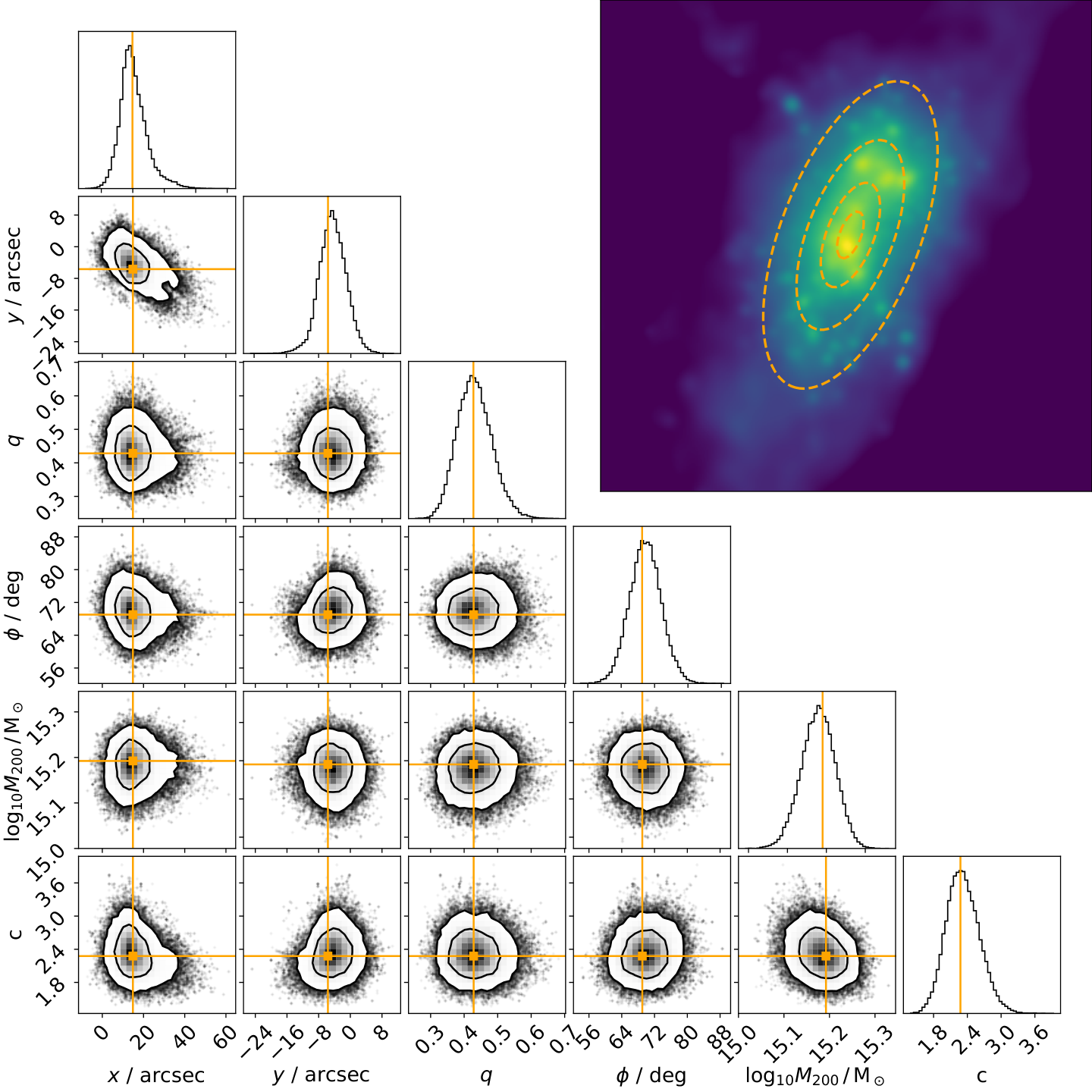
With our likelihood defined, we can now calculate a posterior distribution for the eNFW parameters, given some prior distribution for these parameters. The parameters in question are the and coordinates of the centre of the eNFW, the mass () and concentration () of the eNFW profile, and the axis ratio () and position angle ( – the angle from the -axis to the major axis of the mass distribution). Due to the fact that is ill-defined when , and to avoid complications associated with the periodicity of the parameter , we actually parameterise the eNFW in terms of two components of ellipticity, related to and by
| (8) |
We adopt Gaussian priors on the and coordinates of the halo centre, with a standard deviation of 5 arcmin, centred on the projected location of the most gravitationally bound particle within the galaxy cluster. We adopt a uniform prior on , for values between and , and a uniform prior on in the range 1 to 20. Finally, we adopt uniform priors on each of and in the range -1 to 1, with the additional constraint that .
Using these priors, and the likelihood defined in Equation (7), we use the package emcee (Foreman-Mackey et al. 2013) to perform an MCMC fit to the shear maps from each of our simulated clusters. An example posterior distribution (for one of our CDM haloes) is shown as a corner plot in Fig. 5, with the maximum a posteriori (MAP) model parameters marked in orange. In the top-right of Fig. 5 the convergence map for this cluster is plotted, with iso-convergence contours of the MAP model overlaid in orange. It is clear from this figure that a model with elliptical symmetry is simplistic when compared with the true projected mass distribution of this simulated cluster, owing to features like substructure in the lens that are not captured by the model. Nevertheless, the axis ratio and position angle of the model appear to have a strong correspondence with the projected density map. Also from this figure, we see that with SuperBIT-like data we can determine for an individual cluster to a precision of (the standard deviation of the marginalised posterior in this case). Note that the 100 most massive haloes from each of the CDM and SIDM1 bahamas simulations span a range of halo masses of approximately , and the standard deviation of the posterior distribution is found to increase with decreasing halo mass. For our sample of haloes, the relation between and is well described by .1010 10 This clearly cannot be valid for considerably higher masses, given that would become negative at masses greater than approximately . While we only have 5 clusters with , there is a slight indication that this relationship begins to plateau towards at the high mass end.
SuperBIT’s ability to measure the shapes of individual galaxy clusters with reasonable precision opens up new ways of analysing cluster shapes. In contrast, current ground based weak lensing data – which has a lower number density of usable weak lensing sources – typically requires cluster shear fields to be stacked in order to get a reasonable signal-to-noise ratio. Stacking has clear drawbacks for studies of cluster shapes, because intrinsically elliptical clusters will appear round when stacked, unless some method is employed to align the clusters before stacking. This can be done, for example by assuming that the cluster’s mass distribution is well-aligned with the distribution of cluster member galaxies (see Shin et al. 2018, for example), but then the shape of the stacked cluster mass distribution depends on both the intrinsic shape distribution of clusters and the level of alignment between the DM and stars within clusters. Being able to measure shapes for individual clusters allows things like the misalignment between cluster DM haloes and cluster galaxy distributions to be measured.
Because we fit to noise-free data, the MAP point in the eNFW parameter space takes on a special significance. The MAP parameters are independent of , and correspond to those that we would infer for a particular mass distribution in the limit of infinite signal-to-noise weak lensing data. For the rest of this paper we therefore focus only on the MAP estimates of the axis ratios from the eNFW fits to our mock shear fields.
5.3 Distribution of weak lensing axis ratios
Having fit an eNFW model to the shear field for each of the 100 most massive bahamas-CDM and bahamas-SIDM1 clusters, we show the distribution of axis ratios in Fig. 6. The CDM and SIDM1 distributions are almost indistinguishable, with a value of just , similar to that for the DM axis ratio measured in projection at . We also plot the 2D DM axis ratio measured at – which was already plotted in the left panel of Fig. 4 – such that we can discuss the joint distribution of weak lensing shapes combined with 2D shapes at small radii in Section 5.6.
5.4 On what scale does weak lensing measure the halo shape?
Given that 2D reduced inertia tensor shapes for the DM are different between CDM and SIDM1 (i.e. Fig. 3) it is somewhat disappointing that the distributions of weak lensing shapes do not seem to reflect this difference. To understand why, it is useful to address the question “on what radial scale does weak lensing measure the halo shape?”. Of course there need not be a unique answer to this that is valid for all haloes, because the eNFW fit attempts to describe the complete shear field (and so the complete mass distribution of the cluster) with an axis ratio that is independent of radius, while cluster mass distributions are more complex than this. The fact that the median axis ratios in Fig. 3 vary slightly with radius (especially with SIDM) tells us that individual clusters cannot have axis ratios that are independent of radius, and Fig. 3 overstates how smoothly the axis ratio varies with radius for individual systems, because it is a median of all systems.
To gain some insight into the radial scale on which weak lensing is most sensitive to the halo shape, we compare the axis ratios as a function of radius measured by the 2D inertia tensor, with the weak lensing axis ratios. For each DM model, and at each radius, we have 100 inertia tensor shapes, and the corresponding 100 weak lensing shapes. We calculate the Pearson correlation coefficient, , between these inertia tensor shapes and weak lensing shapes, and plot them as a function of the radius at which the inertia tensor shape was calculated in Fig. 7. The different line styles correspond to different inertia tensor definitions, and it is clear that the weak lensing shape is most correlated with the reduced inertia tensor shape measured at , for which the correlation coefficient is . The fact that cluster weak lensing shapes are most closely related to an inertia tensor shape measured on the scale of (approximately the virial radius of these clusters at z=0.375), while SIDM changes the shape primarily of the inner halo (see Fig. 1 and Fig. 3), explains why the weak lensing axis ratio distributions are so similar between CDM and SIDM1.
It is interesting to note that when measuring the inertia tensor in shells, it is shells at that are the most correlated with the weak lensing shape. This shift towards smaller radii when compared with the reduced inertia tensor is most likely driven by the fact that the contribution of different annuli to the total mass of an NFW cluster () peaks at around the scale radius, which for clusters of this mass is around 500–800. The fact that the reduced inertia tensor outperforms the standard inertia tensor in terms of predicting the weak lensing shape, with a correlation coefficient approaching 1, suggests that the weighting given to different radii by the reduced inertia tensor, roughly matches the weighting of different radii to the overall weak lensing shear field.
We also note that the 2D reduced inertia tensor shapes at and the weak lensing shapes are not just highly correlated, the axis ratios measured by the two methods are approximately the same. For example, with CDM: and , while the standard deviations are and , with a correlation coefficient between the two shape measurements of 0.84. This result – that weak lensing can accurately measure the shape of a halo as it would be measured by a simulator using the inertia tensor – is in contrast with the findings of Harvey et al. 2021, who found that weak lensing inferred axis ratios were typically much rounder than those calculated from the inertia tensor. Specifically, for a definition of ellipticity ,1111 11 This is different from the definition of ellipticity implicit in equation (8), which is they found that .
While we do not know the cause of this difference, there was no particular explanation in 19 for why weak lensing would infer such round shapes for clusters, and we suspect our result (that weak lensing can measure a shape that is closely related to that from the inertia tensor) is correct. Differences between our work and 19 include a significantly smaller field-of-view in 19 (only out to about 40% of the virial radius), and the use of so-called pseudo-elliptical NFW (pNFW) mass distributions. A pNFW is similar to an eNFW, in that it starts off with a spherically symmetric NFW profile, however, whereas the eNFW deforms an NFW into something with elliptical iso-convergence contours, the pNFW has elliptical iso-potential contours instead (Golse & Kneib 2002; Jullo et al. 2007).
The use of pNFW profiles is driven by the deflection angles being easier to compute, but they can sometimes correspond to unusual mass distributions, which can have “dumbbell-shaped” iso-convergence contours, and even regions with negative convergence. That said, Dúmet-Montoya et al. 2012 found that these problems were primarily for large ellipticities, and that for ellipticities typical of simulated halos, pNFW mass distributions can provide an accurate description of an eNFW mass distribution. This means that the use of pNFW profiles is, in and of itself, unlikely to be the cause of the low ellipticities in 19. However, there are various ellipticity definitions in the literature surrounding pNFW profiles, and a conversion must be made between the axis ratio of the iso-potential contours and the axis ratio of the corresponding matter distribution, such that the 19 results could stem from some mismatch in ellipticity definitions when using the pNFW.
5.5 Fitting NFW profiles with radially-varying ellipticity
Given that shape differences are most apparent in the inner halo, but that weak lensing-inferred axis ratios are dominated by the shapes of the outer halo, one possibility for distinguishing between CDM and SIDM1 using halo shapes is to fit a model where the inner and outer halo have separate ellipticities. We implement such a model within PyAutoLens (Nightingale et al. 2021), making use of the fact that PyAutoLens can use a “CSE decomposition” (Oguri 2021) to calculate the deflection angles for elliptical NFW profiles. The idea of the CSE decomposition is to first represent an NFW profile as the sum of many cored steep ellipsoid (CSE) profiles. In projection, a CSE profile has a constant surface density at small radii, which then turns over (at a radius that we call ) to fall off as at large radii, details are in Oguri 2021.
Oguri 2021 showed that 44 CSE profiles could represent an NFW density profile to a fractional accuracy of 1 part in over the full range of radial scales that we are interested in, and this particular CSE decomposition (Oguri 2021, for which the coefficients can be found in Table 1 of) is the one that we use here. The advantage of using many CSEs instead of an NFW profile, comes when one wishes to make the projected mass distribution elliptical. This is because the deflection angle field due to an elliptical NFW profile requires computationally expensive numerical integrals to be performed, whereas the deflection angles due to each CSE are analytic. As such, using a CSE decomposition can speed up deflection angle calculations for eNFW profiles by over two orders of magnitude when compared with the standard approach.
While not the originally intended purpose of the CSE decomposition, another potential benefit is the flexibility to have more complex angular structure than a radially-independent axis ratio and position angle. Each CSE has an associated , and by varying the axis ratio and/or position angle of the CSEs in a systematic way with the core radius, one can achieve NFW-like profiles which have a radially dependent axis ratio and/or have ‘twists’ in the iso-convergence contours. Here we try one very simple version of this, having separate axis ratios and position angles for the inner and outer halo. Specifically, we add two new parameters to the six of the eNFW profile: and , which are the two components of the ellipticity of the inner halo, related to the axis ratio and position angle of the inner halo through eq. (8). We call this model mass distribution an eInOutNFW profile.
We show an example of fitting this model to a mock cluster shear field in Fig. 8, where we adopted a transition radius between the inner and outer halo of . All CSEs with had an ellipticity set by and , while CSEs with larger had an ellipticity given by and (plotted as and in Fig. 8). Note that while one could allow to also be a free parameter in the fit, we found that degeneracies between parameters in the resulting posteriors made them hard to interpret.
There are a couple of noteworthy comments to make about Fig. 8. The first is that with SuperBIT-like data, the posterior distribution covers all possible inner ellipticities (). This means that such a model is not actually something that could be constrained with weak lensing data alone, and instead would require data more sensitive to the mass distribution on small scales, which could potentially come from strong lensing in the cluster core. The second observation we wish to make is that the eInOutNFW model does not produce a system with elliptical iso-convergence contours (i.e. the orange dashed lines in Fig. 8). This is because each CSE contributes at a range of radii, and so at any given radius the mass distribution comes from a sum of profiles with different axis ratios and position angles.

Even though the inner halo ellipticity parameters cannot be constrained from weak lensing data, it is nevertheless informative to look at the MAP parameters from our fits (because the mock shear field is noise free, and so the MAP parameters are a statement about the best-fit model to the shear field due to the intrinsic mass distribution). In Fig. 9 we plot the distributions of inner and outer axis ratios, using . The distributions of and are not well approximated as Gaussian, and so -- unlike in some previous figures -- we use kernel density estimation1212 12 We used sklearn.neighbors.KernelDensity (Pedregosa et al. 2011), with kernel=‘gaussian’ and bandwidth=0.06. to visualise the distributions. We stress that the results for individual haloes were not very stable, in that they change quite considerable as is varied. However, it is encouraging that the behaviour seems to align with expectations, with distributions of outer axis ratios that are similar between CDM and SIDM1, but with an excess of SIDM1 systems that have . Note that in both CDM and SIDM1 there are systems with quite extreme inner axis ratios (). Visual inspection of the convergence maps for these systems reveal them to be bimodal systems, with two distinct density peaks in the inner regions of the cluster.
5.6 Discussion of using the eInOutNFW profile
The eInOutNFW could be used as a cluster-scale mass model, with the ability to reveal information about the DM cross-section through the distribution of the inner halo axis ratios. The envisioned usage, would be for observational studies that try to fit to combined strong and weak lensing (Niemiec et al. 2020, for example, using the hybrid-Lenstool software). Such software assumes there is a single mass distribution that can explain both the observed strong and weak lensing, so if realistic mass distributions can have radially dependent ellipticities, it would be good to enable such mass distributions within the modelling.
That said, with the specific goal of constraining SIDM using cluster shapes, it is not clear that a single mass model to simultaneously explain both strong and weak lensing data is actually required. Returning our attention to Fig. 6, we see that the shape of the projected mass distribution on small () scales is almost completely uncorrelated with the weak lensing shape. As such, one does not gain much constraining power between CDM and SIDM1 by adding in weak lensing information, above what can be inferred from the 2D shape at alone. If we take the 2D shape at to be a proxy for what one would infer from fitting to strong lensing data, then inferring the shape of the inner halo by fitting to strong lensing data alone may be just as good as building a single model for the mass distribution that has a radially varying ellipticity, and fitting to combined strong and weak lensing data. With that somewhat pessimistic note about the role of weak lensing for this particular science case, we leave an investigation into using strong lensing cluster shapes as a probe of SIDM to future work.
6 Conclusions
We used a set of cosmological hydrodynamical simulations run with two different DM models – CDM as well as SIDM with – to investigate using the shapes of galaxy clusters as a test of the nature of DM. We used the reduced inertia tensor to measure the 3D minor-to-major axis ratios of the DM, gas and stars within clusters, finding that while DM shapes differed quite strongly (with SIDM leading to rounder DM distributions at the centres of haloes than CDM) the distribution of gas and star axis ratios were similar in the different DM scenarios. Unfortunately, this change in DM axis ratios is not reflected in the axis ratios of the projected mass distribution of clusters as they would be inferred from weak lensing data, primarily because the differences in 3D between CDM and SIDM are washed out somewhat in projection, and because weak lensing measures the halo shapes on roughly the scale of the virial radius, whereas the major differences in DM axis ratio happen in the inner halo. Our key findings can be summarised as:
- •
SIDM makes the DM in the inner regions of galaxy clusters more round, while leaving the shape of the star and gas distributions unchanged.
- •
Despite the distribution of stellar axis ratios being the same in CDM and SIDM, information about the stellar shapes of galaxy clusters used in conjunction with the corresponding DM shapes make it easier to distinguish between these two DM models than DM shapes alone.
- •
The differences between the distributions of DM shapes in CDM and SIDM are less pronounced in 2D projection than in 3D.
- •
Balloon-borne imaging from the SuperBIT telescope should be able to measure the axis ratio of individual galaxy clusters, with a precision of approximately for clusters with a mass of , and a greater precision for more massive clusters.
- •
The distribution of weak-lensing-inferred axis ratios is the same in CDM and SIDM. The primary driver of this is that cluster weak lensing measures the shape on a scale of , whereas the shape differences are most apparent at .
Having found that the simple procedure of fitting elliptical NFW profiles to the shear fields of clusters could not distinguish between CDM and SIDM, we introduced a more complex model, where the ellipticity of a cluster’s mass distribution can be different at small and large radii. We found that when fitting this model to CDM and SIDM clusters, the distribution of inner axis ratios was shifted towards unity (meaning more round) in SIDM compared with CDM, as expected. However, weak lensing data alone would be insufficient to constrain the inner axis ratio with any meaningful precision, and so fitting this model would most likely require constraints from strong lensing data in order to distinguish between CDM and SIDM using the distribution of galaxy cluster shapes.
Data Availability
The data underlying this article will be shared on reasonable request to the corresponding author.
Acknowledgments
The authors thank Ellen Sirks, Kyle Oman, Richard Massey, Carlos Frenk, Spencer Everett, Jason Rhodes and David Harvey for helpful discussions. This research was carried out at the Jet Propulsion Laboratory, California Institute of Technology, under a contract with the National Aeronautics and Space Administration (80NM0018D0004). AR was supported in part by NASA grant 14-APRA14-0013 and acknowledges the support of the SuperBIT team. The High Performance Computing resources used in this investigation were provided by funding from the JPL Information and Technology Solutions Directorate.
The bahamas-SIDM simulations used in this work were run on the DiRAC@Durham facility, managed by the Institute for Computational Cosmology on behalf of the STFC DiRAC HPC Facility (www.dirac.ac.uk). The equipment was funded by BEIS capital funding via STFC capital grants ST/K00042X/1, ST/P002293/1, ST/R002371/1 and ST/S002502/1, Durham University and STFC operations grant ST/R000832/1. DiRAC is part of the National e-Infrastructure.
This work made use of the following software packages: Astropy (Astropy Collaboration et al. 2013; Price-Whelan et al. 2018), Corner (Foreman-Mackey 2016), emcee (Foreman-Mackey et al. 2013), Matplotlib (Hunter 2007), NumPy (van der Walt et al. 2011), PyAutoLens (Nightingale et al. 2021), and Scipy (Jones et al. 01).
©2022. California Institute of Technology. Government sponsorship acknowledged.
References
- Agrawal et al. (2017) Agrawal P., Cyr-Racine F.-Y., Randall L., Scholtz J., 2017, J. Cosmology Astropart. Phys., 2017, 022
- Allgood et al. (2006) Allgood B., Flores R. A., Primack J. R., Kravtsov A. V., Wechsler R. H., Faltenbacher A., Bullock J. S., 2006, MNRAS, 367, 1781
- Andrade et al. (2022) Andrade K. E., Fuson J., Gad-Nasr S., Kong D., Minor Q., Roberts M. G., Kaplinghat M., 2022, MNRAS, 510, 54
- Astropy Collaboration et al. (2013) Astropy Collaboration et al., 2013, A&A, 558, A33
- Bett et al. (2007) Bett P., Eke V., Frenk C. S., Jenkins A., Helly J., Navarro J., 2007, MNRAS, 376, 215
- Bondarenko et al. (2021) Bondarenko K., Sokolenko A., Boyarsky A., Robertson A., Harvey D., Revaz Y., 2021, J. Cosmology Astropart. Phys., 2021, 043
- Booth & Schaye (2009) Booth C. M., Schaye J., 2009, MNRAS, 398, 53
- Brinckmann et al. (2018) Brinckmann T., Zavala J., Rapetti D., Hansen S. H., Vogelsberger M., 2018, MNRAS, 474, 746
- Dalla Vecchia & Schaye (2008) Dalla Vecchia C., Schaye J., 2008, MNRAS, 387, 1431
- Despali et al. (2017) Despali G., Giocoli C., Bonamigo M., Limousin M., Tormen G., 2017, MNRAS, 466, 181
- Despali et al. (2022) Despali G., Walls L. G., Vegetti S., Sparre M., Vogelsberger M., Zavala J., 2022, MNRAS, 516, 4543
- Duchi (2016) Duchi J. C., 2016.
- Dúmet-Montoya et al. (2012) Dúmet-Montoya H. S., Caminha G. B., Makler M., 2012, A&A , 544, A83
- Eckert et al. (2022) Eckert D., Ettori S., Robertson A., Massey R., Pointecouteau E., Harvey D., McCarthy I. G., 2022, arXiv e-prints, p. arXiv:2205.01123
- Feng et al. (2017) Feng Y., Hand N., biweidai 2017, rainwoodman/pmesh 0.1.33, doi:10.5281/zenodo.1051254, https://doi.org/10.5281/zenodo.1051254
- Foreman-Mackey (2016) Foreman-Mackey D., 2016, JOSS, 1
- Foreman-Mackey et al. (2013) Foreman-Mackey D., Hogg D. W., Lang D., Goodman J., 2013, PASP , 125, 306
- Golse & Kneib (2002) Golse G., Kneib J. P., 2002, A&A , 390, 821
- Harvey et al. (2021) Harvey D., Robertson A., Tam S.-I., Jauzac M., Massey R., Rhodes J., McCarthy I. G., 2021, MNRAS, 500, 2627
- Hinshaw et al. (2013) Hinshaw G., et al., 2013, ApJS , 208, 19
- Hunter (2007) Hunter J. D., 2007, Comput Sci Eng, 9, 90
- Jing & Suto (2002) Jing Y. P., Suto Y., 2002, ApJ, 574, 538
- Jones et al. (01 ) Jones E., Oliphant T., Peterson P., et al., 2001–, SciPy: Open source scientific tools for Python, http://www.scipy.org/
- Jullo et al. (2007) Jullo E., Kneib J. P., Limousin M., Elíasdóttir Á., Marshall P. J., Verdugo T., 2007, New Journal of Physics, 9, 447
- Kaplinghat et al. (2014) Kaplinghat M., Keeley R. E., Linden T., Yu H.-B., 2014, Phys. Rev. Lett. , 113, 021302
- Kaplinghat et al. (2016) Kaplinghat M., Tulin S., Yu H.-B., 2016, Phys. Rev. Lett. , 116, 041302
- Kullback & Leibler (1951) Kullback S., Leibler R. A., 1951, The Annals of Mathematical Statistics, 22, 79
- Leauthaud et al. (2007) Leauthaud A., et al., 2007, ApJS , 172, 219
- Lotz et al. (2017) Lotz J. M., et al., 2017, ApJ, 837, 97
- McCarthy et al. (2017) McCarthy I. G., Schaye J., Bird S., Le Brun A. M. C., 2017, MNRAS, 465, 2936
- McCarthy et al. (2018) McCarthy I. G., Bird S., Schaye J., Harnois-Deraps J., Font A. S., van Waerbeke L., 2018, MNRAS, 476, 2999
- McDaniel et al. (2021) McDaniel A., Jeltema T., Profumo S., 2021, J. Cosmology Astropart. Phys., 2021, 020
- Miralda-Escudé (2002) Miralda-Escudé J., 2002, ApJ, 564, 60
- More et al. (2011) More S., Kravtsov A. V., Dalal N., Gottlöber S., 2011, ApJS , 195, 4
- Navarro et al. (1997) Navarro J. F., Frenk C. S., White S. D. M., 1997, ApJ, 490, 493
- Nesseris & García-Bellido (2013) Nesseris S., García-Bellido J., 2013, J. Cosmology Astropart. Phys., 2013, 036
- Niemiec et al. (2020) Niemiec A., Jauzac M., Jullo E., Limousin M., Sharon K., Kneib J.-P., Natarajan P., Richard J., 2020, MNRAS, 493, 3331
- Nightingale et al. (2021) Nightingale J. W., et al., 2021, J. Open Source Softw., 6, 2825
- Oguri (2021) Oguri M., 2021, PASP , 133, 074504
- Oguri et al. (2010) Oguri M., Takada M., Okabe N., Smith G. P., 2010, MNRAS, 405, 2215
- Pedregosa et al. (2011) Pedregosa F., et al., 2011, Journal of Machine Learning Research, 12, 2825
- Peter et al. (2013) Peter A. H. G., Rocha M., Bullock J. S., Kaplinghat M., 2013, MNRAS, 430, 105
- Postman et al. (2012) Postman M., et al., 2012, ApJS , 199, 25
- Price-Whelan et al. (2018) Price-Whelan A. M., et al., 2018, AJ, 156, 123
- Ren et al. (2019) Ren T., Kwa A., Kaplinghat M., Yu H.-B., 2019, Physical Review X, 9, 031020
- Robertson et al. (2017) Robertson A., Massey R., Eke V., 2017, MNRAS, 465, 569
- Robertson et al. (2019) Robertson A., Harvey D., Massey R., Eke V., McCarthy I. G., Jauzac M., Li B., Schaye J., 2019, MNRAS, 488, 3646
- Rocha et al. (2013) Rocha M., Peter A. H. G., Bullock J. S., Kaplinghat M., Garrison-Kimmel S., Oñorbe J., Moustakas L. A., 2013, MNRAS, 430, 81
- Romualdez et al. (2018) Romualdez L. J., et al., 2018, in Evans C. J., Simard L., Takami H., eds, Society of Photo-Optical Instrumentation Engineers (SPIE) Conference Series Vol. 10702, Ground-based and Airborne Instrumentation for Astronomy VII. p. 107020R (arXiv:1807.02887), doi:10.1117/12.2307754
- Sagunski et al. (2021) Sagunski L., Gad-Nasr S., Colquhoun B., Robertson A., Tulin S., 2021, J. Cosmology Astropart. Phys., 2021, 024
- Schaye & Dalla Vecchia (2008) Schaye J., Dalla Vecchia C., 2008, MNRAS, 383, 1210
- Schaye et al. (2010) Schaye J., et al., 2010, MNRAS, 402, 1536
- Schneider et al. (2012) Schneider M. D., Frenk C. S., Cole S., 2012, J. Cosmology Astropart. Phys., 2012, 030
- Shaaban et al. (2022) Shaaban M. M., et al., 2022, arXiv e-prints, p. arXiv:2210.09182
- Shin et al. (2018) Shin T.-h., Clampitt J., Jain B., Bernstein G., Neil A., Rozo E., Rykoff E., 2018, MNRAS, 475, 2421
- Springel (2005) Springel V., 2005, MNRAS, 364, 1105
- Springel et al. (2001) Springel V., White S. D. M., Tormen G., Kauffmann G., 2001, MNRAS, 328, 726
- Tam et al. (2022) Tam S.-I., Umetsu K., Robertson A., McCarthy I. G., 2022, arXiv e-prints, p. arXiv:2207.03506
- Wiersma et al. (2009a) Wiersma R. P. C., Schaye J., Smith B. D., 2009a, MNRAS, 393, 99
- Wiersma et al. (2009b) Wiersma R. P. C., Schaye J., Theuns T., Dalla Vecchia C., Tornatore L., 2009b, MNRAS, 399, 574
- van der Walt et al. (2011) van der Walt S., Colbert S. C., Varoquaux G., 2011, Comput Sci Eng, 13, 22
Appendix A Analytically projecting 3D shapes to 2D shapes
Imagine that we have some 3D mass distribution, with inertia tensor which has eigenvalues , and . Without loss of generality, let’s assume that the associated eigenvectors are along the , and -axes, respectively (so the major axis is the -axis and the minor axis is the -axis). If we imagine that the mass distribution giving rise to the inertia tensor is a multivariate Gaussian distribution of equal mass particles, then the density of particles (up to some overall normalisation) is entirely specified by .
To project this mass distribution along some line-of-sight, , we need to find the positions of particles along two axes orthogonal to the axis, which we label and , with associated unit vectors and . The variance of particle positions along the axis will be , and that along the axis will be . Similarly the covariance between and coordinates of particles will be . The 2D inertia tensor of the projected particle distribution is simply
| (9) |
We can find the eigenvalues of , which we call and . Then the 2D axis ratio is .