Mangrove: Learning Galaxy Properties from Merger Trees
Abstract
Efficiently mapping baryonic properties onto dark matter is a major challenge in astrophysics.
Although semi-analytic models (SAMs) and hydrodynamical simulations have made impressive advances in reproducing galaxy observables across cosmologically significant volumes, these methods still require significant computation times, representing a barrier to many applications. Graph Neural Networks (GNNs) have recently proven to be the natural choice for learning physical relations. Among the most inherently graph-like structures found in astrophysics are the dark matter merger trees that encode the evolution of dark matter halos. In this paper we introduce a new, graph-based emulator framework, Mangrove, and show that it emulates the galactic stellar mass, cold gas mass and metallicity, instantaneous and time-averaged star formation rate, and black hole mass —as predicted by a SAM— with root mean squared error up to two times lower than other methods across a simulation box in 40 seconds, 4 orders of magnitude faster than the SAM. We show that Mangrove allows for quantification of the dependence of galaxy properties on merger history. We compare our results to the current state of the art in the field and show significant improvements for all target properties. Mangrove is publicly available.11
1
https://github.com/astrockragh/Mangrove
I Introduction
In the hierarchical paradigm of CDM cosmology, dark matter is a crucial constituent of galaxy formation. While modeling the evolution of universes with only dark matter can be done both analytically (Sheth et al. 2001) or through numerical N-body simulations (Aarseth et al. 1979; Efstathiou et al. 1985; Maksimova et al. 2021), co-evolving dark matter and baryons still represents a major challenge, as no simple, direct mapping between the two exists (Contreras et al. 2015; de Santi et al. 2022). Instead we turn to simulations for modeling these complex interactions. Two widely accepted frameworks for doing so are semi-analytic models (SAMs) and hydrodynamic simulations, which in the last two decades have made it possible to populate cosmologically significant volumes with galaxies (Somerville et al. 2008; Vogelsberger et al. 2014; Somerville & Davé 2015; Naab & Ostriker 2017; Vogelsberger et al. 2020). However, the state-of-the-art hydrodynamical simulations take hundereds of millions of CPU hours to run (Schaye et al. 2015; Pillepich et al. 2018; Davé et al. 2019; Villaescusa-Navarro et al. 2021). SAMs achieve much greater computational efficiency by combining dark matter merger trees with a suite of physically motivated recipes for evolving the baryonic components of galaxies, but still require several hundreds of CPU hours to fill a simulation box (White & Frenk 1991; Cole et al. 1994; Somerville & Primack 1999; Benson 2012; Lacey et al. 2016; Lagos et al. 2018). Both methods reproduce many key observables over a broad redshift range, and semi-analytic and numerical hydrodynamic simulations make qualitatively similar predictions for many galaxy properties (Somerville & Davé 2015), as well as agreeing halo-by-halo on stellar and interstellar medium (ISM) properties (Pandya et al. 2020; Ayromlou et al. 2021; Gabrielpillai et al. 2021).
However, there are still significant differences between SAMs and hydrodynamic simulations, as well as tension between the behavior of individual SAMs and hydrodynamic simulations (Somerville & Davé 2015). This tension is seen both on a halo-by-halo basis and on a population-basis, depending on the parameter in question.
Kamdar et al. 2016; Agarwal et al. 2018; Jo & Kim 2019; Lovell et al. 2022; de Santi et al. 2022(hereafter K16a, A18, JK19, L22, dS22) all attempt to map between dark matter and galactic baryonic properties using simple ML algorithms, like Extremely Randomized Trees, Random Forests, Multi-Layer Perceptrons or a combination of the above. These all attempt to map between dark matter halos and galactic properties using only features from the final halos at , or summary statistics believed to encode the merger history along with the features of the halo. These methods all achieve reasonable success on select quantities such as galactic stellar mass and hot gas mass, but struggle to reconstruct quantities such as cold gas mass, star formation rate (SFR), and metallicity. Even in cases where the regression methods were able to predict the median values of a quantity with relatively low error (such as stellar mass), these techniques typically underestimated the dispersion in the baryonic property at a given halo mass (Agarwal et al. 2018). Galaxy properties such as stellar mass, ISM mass, stellar and ISM metallicity and SFR are known to lie in a relatively small sub-region of the high-dimensional parameter space; i.e., they populate a hyperplane. The ultimate goal of emulation methods is to reproduce the full hyperplane and its dispersion for the full suite of baryonic properties of interest.
In this work, we present a new method for learning this highly non-trivial mapping, using the natural choice for learning on merger trees, a Graph Neural Network (GNN). GNNs have lately been demonstrated to work extremely well at modeling various problems in astrophysics (Cranmer et al. 2019; Cranmer
et al. 2020; Cranmer
et al. 2021a; Cranmer
et al. 2021b; Villanueva-Domingo et al. 2021; Thiele et al. 2022; Lemos et al. 2022, e.g.,). This choice of model allows us to include the full merger history as recorded in the merger tree, since the merger tree can naturally be encoded as a graph.
As we will show, our model, Mangrove, outperforms all other models in the literature when predicting stellar mass, cold gas mass, black hole mass, cold gas metallicity, and SFR.22 2 In addition to these 5, we also include SFR averaged over 100 Myr as a target variable. This indicates that exploiting the inherent structure of the merger tree indeed is the stronger choice for mapping directly between dark matter and baryonic properties. In this paper, we will furthermore demonstrate some valuable use cases that Mangrove allows for. First, we can probe the extent to which the exact merger history is important for predicting baryonic quantities, in a way that is infeasible with SAMs and hydrosimulations. Comparing results from using different parts of the merger trees allows us to quantify what aspects of baryonic properties are due to formation history, and which are due to the direct, time-independent dark matter-baryon connection, which has not been possible until now.
We can furthermore probe the importance of halo features along the merger tree in order to determine which parameters would be important in constructing an analytical theory that directly relates the merger tree to galactic properties, and where the most salient information lies. This is done by removing certain parameter sets and observing the change in model performance.
This paper is designed as follows. In §II we present the simulations used to train Mangrove, as well as our data selection criteria. In §III we briefly introduce GNNs and the loss function used for optimizing Mangrove. In §IV we present our results. In §IV.2.1 we present the results for predicting galactic stellar mass at different redshifts. §IV.3 compares our results to the existing literature. §V presents our exploration of the dependence of stellar mass on formation history, as well as an exploration of which dark matter features are most important for. In §VI we discuss our results and possible future work, and in §VII we summarize our conclusions. An appendix with additional details is also provided.
II Simulations and Data
II.1 Simulations and Merger Trees
We use the dark matter only version of the IllustrisTNG simulation, TNG-100-1-Dark. This simulation contains (1820)3 particles within a box of on a side. This implies a dark matter particle mass of h. The halo finding code rockstar (Behroozi et al. 2013a) has been run on 99 snapshots from this simulation, and the consistenttrees (Behroozi et al. 2013b) code is used to construct merger trees from these halo catalogues. See Gabrielpillai et al. 2021 for more details on the halo finding and merger tree algorithms.

II.2 Santa Cruz Semi-Analytic Model
We then run the well-established Santa Cruz Semi-Analytic Model (Somerville & Primack 1999; Somerville et al. 2008; Somerville et al. 2015) on the merger trees described above. The current version of the SC-SAM is documented in G21.
Fundamentally, the SAM uses a set of coupled ODEs to track the flow of matter, gas, and metals between different reservoirs (the diffuse intergalactic medium, hot gas halo, cold gas in the ISM, stars, etc.). The predictions of the SC-SAMs have been extensively compared with observations from , and the SC-SAMs predictions are in good agreement with observables such as stellar mass functions, SFR distributions, and cold gas content (Somerville et al. 2008; Somerville et al. 2015; Yung et al. 2019a; Yung et al. 2019b; Somerville et al. 2021). Moreover, they produce reasonably similar predictions to hydrodynamic simulations for the stellar mass content and cold ISM content of galaxies across a broad range of halo mass and cosmic time. See Somerville & Davé 2015 for a review comparing many SAMs and hydrodynamical simulations, Pandya et al. 2020 for a comparison of the Santa Cruz SAM with the FIRE simulations, and G21 for a comparison of the SC-SAMs with the IllustrisTNG simulations.
The SAM reproduces the galaxy “assembly bias” (dependence of clustering on properties other than halo mass) seen in IllustrisTNG, which is by definition not reproduced by regular Halo Occupation Distribution (HOD) models (Hadzhiyska et al. 2021).
II.3 Data Selection
To ensure that the galaxies in the dataset have reliable features and targets, we employ a set of selection criteria. First, only merger trees where the final halo has a mass of or above are included. This choice is made as the mass of the final halo indicates both the reliability with which the dark matter properties can be measured as well as the reliability of the derived SAM baryonic properties. Secondly, only central galaxies are included, since centrals and satellites are believed to have different relationships with their host halos (Hearin et al. 2016). An inclusion of satellites in future work would be of great interest.
Since in any given merger tree there can be upwards of millions of nodes, some reductions are made. As we are mainly interested in probing the merger history, we preserve nodes/halos that are either:
- •
A progenitor node, i.e., the first time a halo was detected in the simulation
- •
Pre-merger nodes, i.e., halos from the snapshot before they merge
- •
Post-merger nodes, i.e., halos that are the direct result of a merger
- •
The final node, i.e., the final halo
This reduces the number of nodes by a factor of 10-50, depending on the merger tree in question. A sample merger tree resulting from this selection can be seen in Figure 1. Our selection produces a strong inductive bias, since smooth accretion modes are not included. We also limit the total number of nodes to be , which results in the exclusion of 107 merger trees. Since we regress logarithmic targets, only galaxies with non-zero target quantities are included, excluding 470 trees. In total, the dataset consists of 108,338 merger trees. In the future, this problem should be addressed more eloquently, either by combining Mangrove with a classifier predicting if a given galaxy has a zero-value target or not. Another transformation such as the arcsinh transformation could also be considered.
In the basic dataset, we include all dark matter features that are not IDs, x,y,z positions, or x,y,z velocities, even features not explicitly used by the SAM. See §A in the appendix for a list of halo parameters. The description of our training, validation, and test set selection can also be found in §B of the appendix.
SAMs output a large range of baryonic galactic properties, but for exploring the possibility of emulating them with a GNN, we pick a few quantities of interest. The main target of interest is stellar mass (, hereafter ). This is a central quantity for both creating mock catalogues and for simulators to successfully reproduce, and is therefore also the main focus of this project.
To explore the possibility of emulating other baryonic properties that are physically significant or closely related to observables, we also include a range of other targets.
- •
Cold gas (ISM) mass (, hereafter ). The cold gas is the fuel for star formation, and can also be probed observationally through sub-mm emission lines such as CO and through the dust continuum. This is also explored by A18 and L22.
- •
Black hole mass (, hereafter ). The supermassive black hole at the center of a galaxy influences the entire galaxy way beyond its gravitational influence (Kormendy & Ho 2013). This is also explored by JK19 and L22.
- •
Cold gas (ISM) metallicity (, hereafter ). The cold gas metallicity is observable through the strength of different metal lines and is used as a tracer of cold gas clouds. This quantity is also explored by A18 and L22.
- •
Instantaneous Star Formation Rate (, hereafter ). This is also explored by A18, JK19, L22 and dS22.
- •
Star Formation Rate averaged over 100 Myr (, hereafter ). Both SFR properties can be probed through observations of UV or FIR light, and emission lines such as H, and correlate strongly with color. We attempt to regress both the current and 100 Myr averaged SFR, since these in conjunction should provide crucial information about the recent merger history of a galaxy (Caplar & Tacchella 2019; Iyer et al. 2020).
III Graph Neural Networks

The most successful models are the ones which embed well-motivated inductive biases into the model that one wishes to fit to some data. In machine learning, using convolutional neural networks (which preserve locality) for images is a prime example of this general principle. Since halo and galaxy evolution are naturally encoded in merger trees, which are graphs, a Graph Neural Network (GNN) is an intuitive choice for mapping galactic baryonic physics onto dark matter. GNNs, as other ML methods, are built from a sequence of modules, called layers. These layers are then stacked as a sequential series of message-passing or graph convolutional layers (Kipf & Welling 2017; Battaglia et al. 2018) which pass information from the nodes along the edges of the graph, followed by a differentiable pooling function and a decoder function, which is usually a Multi-Layer Perceptron (MLP) (Rumelhart et al. 1986). The pooling function is applied in order to standardize the outputs for graphs varying number of nodes. The overall flow of Mangrove is visualized in Figure 2.
A description of the full structure of Mangrove, known as the architecture of the model, can be found in §E in the appendix.
III.1 Core Concepts
GNNs are a species of neural network which operate on graph-structured data (Scarselli et al. 2008; Bronstein et al. 2017; Battaglia et al. 2018). For our purpose, the graphs, , on which GNNs operate are defined as 2-tuples, ,33 3 We adhere closely to the notation used in Battaglia et al. 2018; Cranmer et al. 2019 for formal definitions. where , and is the total number of nodes, is a set of node attribute vectors of dimensionality . The edges can be encoded by , a set of edge attribute vectors of dimensionality , and with indices of the “receiving” and “sending” nodes connected by the -th edge.
In this work, only node attributes and edge indices are used, although edge features could be created. Note that our graphs are directed, since merger trees are inherently directed in time. A directed graph means that information can only be passed one way on a given edge, which for our purpose follows the flow of time since propagating information backwards in time would break causality.
The neighborhood of node consists of all nodes that are connected to node by an edge. Note that for a directed graph, this only includes the set of nodes for which . Some prefer to instead define two separate notions of neighborhoods for directed graphs, an incoming neighborhood and an outgoing neighborhood. Our definition would be the same as the incoming neighborhood. We denote the neighborhood of node by .
III.2 GraphSAGE
As described above, the message-passing or graph convolutional layer makes up the cornerstone of GNNs. Information from the neighborhood is passed along the edges leading to a given node, in order to learn not just from the node feature vector but from its neighbors.
There has been a variety of different proposed message-passing and graph convolutional layers. In this project we use the PyTorch Geometric (Fey &
Lenssen 2019), implementation of the GraphSAGE convolutional layer from Hamilton
et al. 2017. With each application of this layer, each node updates its state from the input state to a hidden state , through:
| (1) |
where and are learnable weight matrices. Thus, operates on information from the node itself, and on the mean44 4 Although the mean is used here, any other differentiable aggregation function is usable. of the node states of the neighborhood nodes.
In order to gain some intuitive understanding of what this layer actually does, it is useful to think about these layers in terms of function. We can introduce two learnable functions, , the node function and , the neighborhood function, which are both constrained to be linear. Then a full application of GraphSAGE can be written as:
| (2) |
The optimization task can then be framed as learning the functions and , expressed through matrices and . See Figure 2 for a schematic of the flow of these learnable functions.
Since all functions in this layer are linear, a non-linear activation function, usually written as ,55 5 Not to be confused with the scatter or standard deviation. is applied between each layer, allowing expression of nonlinear functions. Thus the node state is updated to:
| (3) |
In this work we use the ReLU activation function between GraphSAGE layers (Agarap 2018).
III.3 Loss Function
The loss function is central to the optimization and performance of any GNN, as the parameter set which makes up the GNN is optimized to satisfy . In this work we employ a generalized Gaussian Negative Log-Likelihood (NLL).
For a single input, the general Gaussian NLL is defined as:
| (4) |
where, is the true target vector, is the network prediction vector, is the predicted covariance matrix, and denotes its determinant. These are then easily extended to their batch form, by simply summing over all inputs in a batch.
In this paper, the quoted results are obtained via a purely diagonal covariance matrix, although in some cases, we obtained better results with the full covariance matrix. The diagonal covariance matrix is preferred for its simplicity, and still renders Gaussian uncertainties, which are highly useful as discussed in §VI. The metrics (see §IV.1) between the two cases differ by no more than a few %. A further discussion of the uncertainties can be found in Appendix §C.
IV Results
In this section, we first introduce the metrics used to characterize the performance of Mangrove. We then present results for our predictions and compare them to other methods and the possibility of generalization across different redshifts. We then explore the predictions of the other target parameters.
We compare our results to results from four other frameworks.
- •
Our prediction will be compared to the more widely used method for connecting halo masses and galactic stellar masses, Abundance Matching (Vale & Ostriker 2004).
- •
Where possible, we compare to other papers in the literature which have attempted to regress the same target parameters. However, these are not performed on the same dataset as ours.
- •
In order to mitigate this issue, we train a MLP on the halos (final halos) of our dataset which should be comparable to the methods in the literature.
- •
As a way of providing an estimate of the best possible performance on the test set, we run the SC-SAM with different random seeds, and calculate the comparison metrics between them. This should be an estimate of the lower information limit. If our predictions do significantly better than this across the entire simulation, it would be cause for some concern. This is not the same as the numerical uncertainty, but arises due to the fact that while the model can learn summary statistics for the probability distributions used in the SAM, it is a fully deterministic model and thus could not emulate the random draws. Going forward this is denominated as the SAM probabilistic limit.
IV.1 Metrics
The most commonly used metric to determine accuracy in astronomy is the scatter66 6 Also commonly referred to as the standard deviation or root-mean-squared-error., defined as:
| (5) |
where is the residual of a single prediction and is the mean of the residuals.
This metric has two significant caveats. Firstly, it does not measure any systematic offset in the residuals. Therefore, as an important addition, we introduce the bias as an auxiliary metric, defined as the mean of the residuals, i.e.:
| (6) |
The bias effectively measures any systematic offset. The best possible predictions would have low scatter and no bias.
Second, because the scatter is susceptible to outliers, we include two secondary metrics that are more stable and not directly optimized for in our loss function.
- •
Pearson correlation coefficient (), i.e., the linear correlation between the target and model prediction:
(7) - •
Coefficient of determination ():
(8)
For both of these metrics, a perfect set of predictions would correspond to
It is important to note that the ability to predict any specific target generally improved when Mangrove was trained to predict all target variables. We therefore distinguish between models trained for all targets and only a single target when presenting results.
IV.2 Stellar Mass Results

As the central quantity of interest, the stellar mass received the most attention in this paper. The test set results were a scatter of 0.070 dex, with 0.002 dex bias. This is shown in Figure 3, along with a comparison to the usual halo mass abundance matching approach.77 7 Other metrics can be found in Table 1 Abundance matching (Vale & Ostriker 2004), simply rank-orders all galaxies and halos by mass and assumes a monotonic matching relation exists between the two. We include this comparison as a baseline due to its simplicity and widespread use.
Figure 3 shows the relation between target value and predicted value, along with distributions on the respective axes. The Figure shows the (target, prediction) - relation as a 2D histogram with logarithmic bin heights. If this relation follows the diagonal, that would indicate perfect predictions. The tighter the relation follows the diagonal, the better.
A few comparisons are beneficial to keep in mind:
- •
Training Mangrove to predict only yields a scatter of 0.078 dex, 11% worse than the performance when training Mangrove to predict all quantities simultaneously.
- •
The performance of the model worsens to a scatter of 0.132 dex when using only the parameters of the final halo, indicating a strong dependence on assembly history.
- •
The scatter of Mangrove’s predictions is comparable to the SAM probabilistic limit as defined above, which has a scatter of 0.043 dex (see Table 1).
Further investigation of the impact of different features and the merger history can be found in §V.
IV.2.1 Stellar mass at other redshifts
A central question for many ML models is to what extent its predictions will generalize. For astrophysical purposes, generalization across redshifts is crucial. We investigated whether Mangrove would perform well at by doing several experiments.
- 1.
Test models trained at a single redshift at redshifts where they were not trained. This in general leads to imprecise and highly biased results.88 8 bias and
- 2.
Train and test models at individual . Mangrove can achieve an accuracy below 0.08 dex at all redshifts as can be seen in Figure 4.
- 3.
Train a general model by pooling training sets at , and testing at . Compared to training and testing at individual redshifts, we obtain similar results at all redshifts.
- 4.
Most surprisingly, by pooling training sets at , and testing at where Mangrove was not trained, we obtain comparable bias and scatter to where Mangrove was trained.
- 5.
Pooling training sets at , and testing at where Mangrove was not trained, we get a relatively inaccurate result as seen in Figure 5.
All experiments in this section were done with models trained to predict only .
Mangrove performs well on all , even learning a smooth transformation for general redshifts if in the interpolative regime. However, it worsens significantly when extrapolating.


IV.2.2 , , , and Results

In general, we observe a weaker dependence on merger history for all other target quantities, but the predictions from using the full merger tree are always significantly better than just using the final halo, as can be seen in Table 1.99 9 This can also easily be seen if comparing Figures 3 and 6 to Figure 15 in the appendix. The regression results for , , , and for a model trained to predict all targets at the same time are visualized in Figure 6. As can be seen, Mangrove generally performs very well but struggles in regions of or . This is due to the two diverging branches in SFR that occur around this value (see Figure 13 in the appendix).
Notably, the predictions are slightly better than the SAM probabilistic limit. Since the predictions are just below this limit, we can interpret the results as having accurately captured a generalizing rule for mapping between the dark matter merger tree and , with little cause for concern.
See §D in the appendix for an in-depth analysis of both the relations between halo mass and the target parameters, as well as the interdependence of the residuals of the target parameters.
IV.3 Comparison to Benchmark
| Target | Paper/Method | [dex] | Bias [dex] | - score | |
|---|---|---|---|---|---|
| Mangrove | 0.070 | 0.002 | 0.997 | 0.994 | |
| Final halo only | 0.132 | 0.003 | 0.990 | 0.980 | |
| A18 | 0.189 | 0.004 | 0.953 | 0.909 | |
| JK19 | 0.162 | 0.027 | 0.991 | 0.982 | |
| dS22 | 0.132 | - | 0.977 | 0.954 | |
| L22 | - | - | 0.924 | - | |
| Abundance Matching | 0.312 | 0.000 | 0.944 | 0.889 | |
| SAM probabilistic limit | 0.043 | 0.000 | 0.999 | 0.997 | |
| Mangrove | 0.161 | -0.009 | 0.954 | 0.909 | |
| Final halo only | 0.182 | 0.001 | 0.941 | 0.885 | |
| L22 | - | - | 0.799 | - | |
| SAM probabilistic limit | 0.096 | 0.000 | 0.983 | 0.967 | |
| Mangrove | 0.127 | -0.001 | 0.975 | 0.950 | |
| Final halo only | 0.175 | -0.013 | 0.951 | 0.904 | |
| JK19 | 0.272 | 0.044 | 0.965 | 0.927 | |
| L22 | - | - | 0.881 | - | |
| SAM probabilistic limit | 0.129 | 0.000 | 0.967 | 0.934 | |
| Mangrove | 0.123 | -0.005 | 0.974 | 0.948 | |
| Final halo only | 0.151 | -0.007 | 0.960 | 0.922 | |
| A18 | 0.160 | 0.004 | 0.860 | 0.739 | |
| SAM probabilistic limit | 0.074 | 0.000 | 0.990 | 0.981 | |
| Mangrove | 0.353 | -0.025 | 0.936 | 0.876 | |
| Final halo only | 0.392 | 0.002 | 0.921 | 0.847 | |
| A18 | 0.433 | -0.014 | 0.745 | 0.555 | |
| JK19 | 0.93 | -0.024 | 0.902 | 0.760 | |
| dS22 | 0.850 | - | 0.652 | 0.094 | |
| L22 | - | - | 0.804 | - | |
| SAM probabilistic limit | 0.230 | 0.000 | 0.973 | 0.947 | |
| Mangrove | 0.347 | 0.022 | 0.938 | 0.879 | |
| Final halo only | 0.388 | 0.003 | 0.922 | 0.849 | |
| SAM probabilistic limit | 0.200 | 0.000 | 0.980 | 0.960 |
To evaluate our performance against the current state-of-the-art in mapping baryonic properties directly onto dark matter, we provide Table 1, containing accuracy metrics1010 10 See beginning of §IV for an overview of the used metrics for this work and others in the literature at .
Although we here compare directly to the literature results, it should be noted that the dS22 report values for specific, instantaneous SFR, sSFR1111 11 Defined as ., which means that their results for just SFR have significantly higher scatter, since this prediction is dominated by the stellar mass prediction.
Since papers from the literature do not report all metrics used here, we provide an estimate for a final-halo-only result, which effectively follows the basic Neural Network approach of dS22. The final halo only accuracy should also be comparable to the approaches using tree-based algorithms, as shown by dS22, so the results of A18, JK19 and L22 should also be comparable.
As described in §IV, we also provide the probabilistic limit of the SAM.
Comparing our results to results from the literature, we see that Mangrove outperforms other models across all categories, as well as showing remarkable improvements for using the full structure compared to only using the properties of the final halo. Especially and show very significant improvements comparing our merger tree approach with the final halo only approach.
V Dependence on assembly history and feature ablation
A key method of investigating ML models is to simply remove certain parts of either the model or the input data, in order to probe the importance of said part. This process is known as ablation. In this section we seek to quantify the impact on our model accuracy by removing parts of the input data. We here investigate two separate cases, in both cases with models trained to predict only at .
- •
The dependence of our model accuracy on the fraction of the merger history included in the input merger trees.
- •
The dependence of our model accuracy on a different sets of input features when given the full merger tree as an input.
These tests investigate what aspects of current galactic stellar masses are due to history, and which are inevitable due to the fundamental physical connection between different aspects of a galaxy and its host halo, and which of these aspects are the most important.
V.1 Dependence on Merger History
In order to quantify the dependence on merger history of our galactic stellar mass prediction, we perform a simple study. For all merger trees, we reduce the number of nodes by some fixed percentage, P, for which we retrain and retest the model. We reduce the number of nodes starting at earlier times (high redshift) by finding the scale factor corresponding to the P’th percentile and then excluding all halos at scale factors lower than this. Here we choose the fixed percentage in order to not bias the results towards lower-mass galaxies, since in our dark matter only simulations, their assembly would only start being recorded at lower redshifts, and their merger trees would thus not be pruned to the same extent if one pruned above a fixed redshift. Our chosen pruning method is illustrated in the difference between Figures 1 and 7. If our prediction scatter using the P’th - percentile reduced tree is as good as when using the full merger trees, it implies that there was no useful information in the P’th percentile highest redshift nodes that is not also contained in the low redshift nodes.

We choose to train and test 25 times for each percentage. We choose to investigate at 0, 50, 75, 85, 95, 99 and 100% of the merger history removed1212 12 Removal of 100% of the merger history corresponds to only using the final halo. Removing 0% corresponds to using the full merger history.. The median and 16th/84th percentile of the test scatters are shown in Figure 8. It is clear that the impact of including more of the merger history is quite significant, with higher relative significance towards halos at lower redshifts.

V.2 Feature Ablation
A GNN can act as a predictor of what features are most important in determining the properties of a galaxy. Say that one would like to test whether some connection between black hole mass and three halo parameters exists. Then one can simply train and test a GNN using said three parameters, and compare the results to when the GNN uses all parameters. Thus, in order to investigate which features are the most important for Mangrove’s -prediction, we choose this simple approach, where we only include certain sets of features during both training and testing of Mangrove.
Besides a series of physically motivated sets of quantities (see Table 2) from analytical approaches in the literature (Rodríguez-Puebla et al. 2016), we also attempt to regress from an empty tree, i.e., a tree with no features. The merger tree then contains no information but that encoded in the geometric structure itself. This approach is less precise than the final halo only regression, but it still outperforms abundance matching.
We observe that if one wishes to use only a single parameter, has a much lower scatter compared to the otherwise most common choice, the halo mass.
The most salient single group of parameters is the NFW profile parameters.1313 13 Closely followed by . The NFW profile information can be encoded either as or and , which together make the NFW concentration parameter . Combining redshift and NFW profile information rendered the most precise prediction using the fewest features.
Some general interpretability methods rely on the same basic principles of ablation to investigate model behavior, such as SHAP values (Lundberg & Lee 2017). SHAP values are however not reliable for GNNs in their current implementation, but only for simpler models, such as Random Forests (Lundberg et al. 2018).
| Features used | ||
|---|---|---|
| All | 0.0776 | 37 |
| Only redshift | 0.1704 | 1 |
| None/Empty tree | 0.2574 | 0 |
| Only mass | 0.1436 | 1 |
| Only NFW1414 14 Navarro-Frenk-White (NFW) profile (Navarro et al. 1997) profile | 0.1082 | 2 |
| Only | 0.1194 | 1 |
| Redshift and NFW profile | 0.0993 | 3 |
VI Discussion and Further Work
In this section we discuss some of the implications of our work and how these connect to possible future work. Among the topics discussed will be the issues with the constituents of star formation, , and , merger history dependence and interpretability, the bias and dispersion in relationships with halo mass, the predicted uncertainties, and how to use Mangrove with other simulations and combining results from Mangrove with observations.
VI.1 , and
Although this paper shows that some highly accurate mappings between dark matter merger trees and baryonic galactic properties exist, there is still significant scatter between the Mangrove and SAM , and . It should, however, be noted that the scatters between different SAM runs due to only random seed variation in these quantities are already quite high (see Table 1).
There were no notable differences in the reconstruction strength between and , which indicates that reconstructing the Star Formation History, as well as the current , are similar tasks to the Mangrove.
As a way of investigating if Mangrove has learned physically meaningful relationships for these target, we test the interdependence of the target residuals. Here we find that the residuals between the two targets and are strongly correlated (see Figure 12 in the appendix), meaning that if Mangrove predicted a too high , it would also predict a too high , analogous to the Kennicutt-Schmidt relation (Kennicutt 1998).
The improvement in these three quantities when going from using only the final halo to the full merger history was smaller than expected, since they are thought to be strongly connected to the merger history of the galaxy (White &
Frenk 1991; Somerville &
Davé 2015; Caplar &
Tacchella 2019). This aspect of galaxy evolution could instead be more strongly connected to their environments, which is not included as an input to Mangrove. An obvious possibility for future work is therefore to include an encoding of the environment. Since Lovell et al. 2022 showed that summary statistics do not make a significant difference, it would perhaps be wise to include the environmental dependence as an additional graph that extends spatially as in Makinen et al. 2022, such that the environmental dependence could be learned. This would naturally lead to including a more explicit subhalo model, with satellites included in the spatial graph. It would then be natural to also predict properties for the satellites.
VI.2 Merger History Dependence and Interpretability
For , in contrast to , and , we find a very strong dependence on the percentage of merger history included, with the importance of including a specific node increasing the closer it is to the (see Figure 8). This is in contrast to the conclusions of McGibbon &
Khochfar 2022, although their modelling framework does not fully use the formation history.
Our analysis of merger history dependence is, however, only preliminary for all parameters but .
The more powerful graph-based framework should facilitate deeper future investigations of the formation history dependence for a wider range of properties.
Another interesting avenue for interpreting the model, could be to investigate the model’s behavior with symbolic regression (Cranmer
et al. 2020), which would lead to a highly interpretable merger history dependence.
A separate but interesting interpretability approach could be to investigate the merger trees from the point of view of unsupervised learning, as in Jespersen
et al. 2020; Hovis-Afflerbach et al. 2021 using either t-SNE or UMAP (Van der Maaten &
Hinton 2008; McInnes
et al. 2018). This would be done in the latent space of Mangrove, as the latent space would be more readily comparable.
VI.3 Additional Physical Relationships
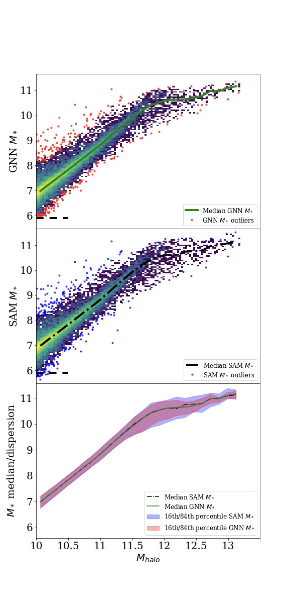
As can be seen in Figure 9, Mangrove reproduces not just the median relationship, but also the dispersion in the relationship. Figure 13 in the appendix shows that this is the case for all quantities except the two ’s. Combining this with the above mentioned correct physical interdependence of the residuals leads to a suspicion that we are closer than ever to being able to emulate the full galaxy property hyperplane. Since Mangrove furthermore performs well at all redshifts, even when interpolating at redshifts where it had not been trained, it is possible to imagine a GNN being able to emulate the full galaxy property hyperplane for all redshifts. Relations like Figure 9 for all other target variables can be found in Appendix §D.
Another curious result is the tendency for Mangrove to improve as more output variables were included (with no increase in the amount of model parameters), indicating that an even larger range of baryonic properties than included here could be predicted by one unified model with even greater accuracy, lending further credence to the possibility of emulating the full galaxy property hyperplane. The authors hypothesize that this is due to weight smoothing, which diminishes spurious correlations, since each weight is “regularized” by the loss from other targets.
VI.4 Uncertainties
As an additional feature in the literature on emulating baryonic physics, we also have some interesting possibilities due to predicting a set of Gaussian covariances. The diagonal entries, the variance of each parameter, could be used as a filter for selecting predictions that Mangrove is highly confident that it has gotten right. For example, if one filter our results such that only the 50% highest confidence regressions as judged by Mangrove were included we get significantly better results (see Table 3, and Figure 16 in the appendix). A further investigation into the drivers behind the variance value is beyond the scope of this paper, but highly valuable information could most likely be extracted from these, as demonstrated by Stiskalek et al. 2022. Distributions and correlations between the predicted uncertainties and galaxy properties can be found in Appendix C.
| Target | Bias | |||
|---|---|---|---|---|
| 0.029 | 0.002 | 0.999 | 0.998 | |
| 0.101 | -0.006 | 0.978 | 0.957 | |
| 0.069 | -0.002 | 0.942 | 0.886 | |
| 0.085 | -0.008 | 0.987 | 0.975 | |
| 0.217 | 0.017 | 0.974 | 0.948 | |
| 0.213 | 0.013 | 0.975 | 0.949 |
A minor drawback to the generalized Gaussian loss function is that information-sparse areas of the target space can end up being “ignored” by Mangrove, which instead prefers ascribing a large variance to these points. An example of this can be seen in the halo mass-stellar mass relation in Figure 9, where low-mass halos with low mass galaxies are effectively ignored in favor of a “safe” floor value of . Since the issue persists in a mass region where the SAM is already quite uncertain due to the mass resolution, and where the galaxies would not currently be of major importance, this is only of minor concern.
VI.5 Extensions to Other Simulations
Mangrove can also be applied to the full magneto-hydrodynamical version of IllustrisTNG, as well as any other SAM and hydrodynamical simulation. An analysis of the dependence of baryonic properties on merger history in IllustrisTNG similar to the one presented in this paper would render crucial information as to how and why SAMs and hydrosimulations render different outputs.
Since Mangrove works regardless of the number of snapshots included, an interesting avenue to explore could also be different subsampling methods, where specific snapshots are left out according to some scheme, whereafter the Mangroves’s performance on the subsampled merger tree is then measured. This would inform decisions about how many snapshots a simulation team needs to store in order to achieve a satisfactory galaxy property reconstruction, possibly reducing the need for storing an extensive number of snapshots.
VI.6 Connection to Observations
While extending our framework to other simulations is exciting, we should consider possibilities for combination with observation. Here it should be noted that as determined in §V, only the recent merger history, which is somewhat possible to observe, is required in order to regress the stellar mass significantly more precisely. This kind of recent merger information should be recoverable from spectroscopic missions (e.g. the PFS Galaxy Evolution Survey (Takada et al. 2014)), since recently merged galaxies can normally be identified from either a strong infrared emission from heated dust, A-star population or kinematics (Kennicutt & Evans 2012). Furthermore, we have determined that the most salient information comes from NFW profile information, which is becoming possible to measure (Niikura et al. 2015). Halo masses are measurable both from dynamic masses but most confidently from lensing. Therefore, one can imagine a simple population-level version of the model developed in this work being used along with measured stellar masses, recent merger histories and halo features to see if the connections that are emphasized by Mangrove truly are the most important.
VII Conclusion
Using the full merger history, we greatly improve upon the current state of the art for emulating galaxy properties with only dark matter properties. We have furthermore shown that interrogating Mangrove renders physical insights into the connection between merger trees and galaxy properties.
Considering first only the models use as an emulator, three points are crucial:
- •
Mangrove outperforms all other known ML models when emulating the SC-SAM , , , , and by using the full merger history of a given galaxy. Predictions always improve when using the full merger history, and especially and are regressed highly accurately when using the merger history. Since and are regressed so well, they do not just reproduce median relationships, but also the width of the distributions.
- •
When trained, Mangrove is respectively 4 and 9 orders of magnitude faster than the SC-SAM and IllustrisTNG. Including training, this drops to respectively 2 and 7 orders of magnitude. Especially for populating large boxes (side length ), this would drastically reduce run times.
- •
Mangrove works at a range of redshifts and can reliably interpolate between redshifts, even if not trained on galaxies at a given redshift.
The physical insights that we have obtained from the model center around two aspects of the connection between merger trees and galactic stellar masses. First, whether the galactic stellar masses are directly related to the properties of the halo within which it resides, or the formation history of the halo, and secondly, which dark matter features are the most valuable. Here we found three especially exciting results.
- •
The earliest half of the merger history of a galaxy can be discarded with only a minor loss of performance when predicting stellar mass.
- •
Including just 1% of the merger history closest to the present day leads to significantly improved regression.
- •
Mangrove identifies one especially important set of features, which encode the halos 1-dimensional NFW profile. This can be encoded in two ways, either by using , , and or and . The second most important parameter is .
References
- Aarseth et al. (1979) Aarseth S. J., Gott J. R. I., Turner E. L., 1979, ApJ, 228, 664
- Abadi et al. (2016) Abadi M., et al., 2016, in 12th USENIX Symposium on Operating Systems Design and Implementation (OSDI 16). pp 265–283
- Agarap (2018) Agarap A. F., 2018, arXiv preprint arXiv:1803.08375
- Agarwal et al. (2018) Agarwal S., Davé R., Bassett B. A., 2018, MNRAS, 478, 3410
- Ayromlou et al. (2021) Ayromlou M., Nelson D., Yates R. M., Kauffmann G., Renneby M., White S. D. M., 2021, MNRAS, 502, 1051
- Ba et al. (2016) Ba J. L., Kiros J. R., Hinton G. E., 2016, Layer Normalization (arXiv:1607.06450)
- Battaglia et al. (2018) Battaglia P. W., et al., 2018, arXiv e-prints, p. arXiv:1806.01261
- Behroozi et al. (2013a) Behroozi P. S., Wechsler R. H., Wu H.-Y., 2013a, ApJ, 762, 109
- Behroozi et al. (2013b) Behroozi P. S., Wechsler R. H., Wu H.-Y., Busha M. T., Klypin A. A., Primack J. R., 2013b, ApJ, 763, 18
- Benson (2012) Benson A. J., 2012, New Astronomy, 17, 175
- Bronstein et al. (2017) Bronstein M. M., Bruna J., LeCun Y., Szlam A., Vandergheynst P., 2017, IEEE Signal Processing Magazine, 34, 18
- Caplar & Tacchella (2019) Caplar N., Tacchella S., 2019, MNRAS, 487, 3845
- Cole et al. (1994) Cole S., Aragon-Salamanca A., Frenk C. S., Navarro J. F., Zepf S. E., 1994, MNRAS, 271, 781
- Contreras et al. (2015) Contreras S., Baugh C. M., Norberg P., Padilla N., 2015, MNRAS, 452, 1861
- Cranmer et al. (2019) Cranmer M. D., Xu R., Battaglia P., Ho S., 2019, arXiv e-prints, p. arXiv:1909.05862
- Cranmer et al. (2020) Cranmer M., Sanchez-Gonzalez A., Battaglia P., Xu R., Cranmer K., Spergel D., Ho S., 2020, arXiv e-prints, p. arXiv:2006.11287
- Cranmer et al. (2021a) Cranmer M., Melchior P., Nord B., 2021a, arXiv:2106.09761 [astro-ph], pp 1–13
- Cranmer et al. (2021b) Cranmer M., Kreisch C., Pisani A., Villaescusa-Navarro F., Spergel D. N., Ho S., 2021b, ICLR 2021 SimDL Workshop, p. 10
- Davé et al. (2019) Davé R., Anglés-Alcázar D., Narayanan D., Li Q., Rafieferantsoa M. H., Appleby S., 2019, MNRAS, 486, 2827
- Efstathiou et al. (1985) Efstathiou G., Davis M., White S. D. M., Frenk C. S., 1985, ApJS, 57, 241
- Fey & Lenssen (2019) Fey M., Lenssen J. E., 2019, in ICLR Workshop on Representation Learning on Graphs and Manifolds.
- Foreman-Mackey (2016) Foreman-Mackey D., 2016, The Journal of Open Source Software, 1, 24
- Gabrielpillai et al. (2021) Gabrielpillai A., Somerville R. S., Genel S., Rodriguez-Gomez V., Pandya V., Yung L. Y. A., Hernquist L., 2021, arXiv e-prints, p. arXiv:2111.03077
- Hadzhiyska et al. (2021) Hadzhiyska B., Liu S., Somerville R. S., Gabrielpillai A., Bose S., Eisenstein D., Hernquist L., 2021, MNRAS, 508, 698
- Hamilton et al. (2017) Hamilton W. L., Ying R., Leskovec J., 2017, arXiv e-prints, p. arXiv:1706.02216
- Harris et al. (2020) Harris C. R., et al., 2020, Nature, 585, 357
- Hearin et al. (2016) Hearin A. P., Zentner A. R., van den Bosch F. C., Campbell D., Tollerud E., 2016, MNRAS, 460, 2552
- Hovis-Afflerbach et al. (2021) Hovis-Afflerbach B., Steinhardt C. L., Masters D., Salvato M., 2021, ApJ, 908, 148
- Hunter (2007) Hunter J. D., 2007, Computing in Science & Engineering, 9, 90
- Iyer et al. (2020) Iyer K. G., et al., 2020, MNRAS, 498, 430
- Jespersen et al. (2020) Jespersen C. K., Severin J. B., Steinhardt C. L., Vinther J., Fynbo J. P. U., Selsing J., Watson D., 2020, ApJ, 896, L20
- Jo & Kim (2019) Jo Y., Kim J.-h., 2019, MNRAS, 489, 3565
- Kamdar et al. (2016) Kamdar H. M., Turk M. J., Brunner R. J., 2016, MNRAS, 455, 642
- Kennicutt (1998) Kennicutt Robert C. J., 1998, ApJ, 498, 541
- Kennicutt & Evans (2012) Kennicutt R. C., Evans N. J., 2012, ARA&A, 50, 531
- Kingma & Ba (2017) Kingma D. P., Ba J., 2017, Adam: A Method for Stochastic Optimization (arXiv:1412.6980)
- Kipf & Welling (2017) Kipf T. N., Welling M., 2017, Semi-Supervised Classification with Graph Convolutional Networks (arXiv:1609.02907)
- Kluyver et al. (2016) Kluyver T., et al., 2016, in Loizides F., Schmidt B., eds, Positioning and Power in Academic Publishing: Players, Agents and Agendas. pp 87 – 90
- Kormendy & Ho (2013) Kormendy J., Ho L. C., 2013, ARA&A, 51, 511
- Kuhn & Johnson (2013) Kuhn M., Johnson K., 2013, Applied predictive modeling. statistics Vol. 26, Springer
- Lacey et al. (2016) Lacey C. G., et al., 2016, MNRAS, 462, 3854
- Lagos et al. (2018) Lagos C. d. P., Tobar R. J., Robotham A. S. G., Obreschkow D., Mitchell P. D., Power C., Elahi P. J., 2018, MNRAS, 481, 3573
- Lemos et al. (2022) Lemos P., Jeffrey N., Cranmer M., Battaglia P., Ho S., 2022, In submission, PNAS
- Lovell et al. (2022) Lovell C. C., Wilkins S. M., Thomas P. A., Schaller M., Baugh C. M., Fabbian G., Bahé Y., 2022, MNRAS, 509, 5046
- Lundberg & Lee (2017) Lundberg S., Lee S.-I., 2017, arXiv e-prints, p. arXiv:1705.07874
- Lundberg et al. (2018) Lundberg S. M., Erion G. G., Lee S.-I., 2018, arXiv e-prints, p. arXiv:1802.03888
- Makinen et al. (2022) Makinen T. L., Charnock T., Lemos P., Porqueres N., Heavens A., Wandelt B. D., 2022, arXiv e-prints, p. arXiv:2207.05202
- Maksimova et al. (2021) Maksimova N. A., Garrison L. H., Eisenstein D. J., Hadzhiyska B., Bose S., Satterthwaite T. P., 2021, MNRAS, 508, 4017
- McGibbon & Khochfar (2022) McGibbon R. J., Khochfar S., 2022, MNRAS, 513, 5423
- McInnes et al. (2018) McInnes L., Healy J., Melville J., 2018, arXiv preprint arXiv:1802.03426
- Naab & Ostriker (2017) Naab T., Ostriker J. P., 2017, ARA&A, 55, 59
- Navarro et al. (1997) Navarro J. F., Frenk C. S., White S. D. M., 1997, ApJ, 490, 493
- Niikura et al. (2015) Niikura H., Takada M., Okabe N., Martino R., Takahashi R., 2015, Publications of the Astronomical Society of Japan, 67, 103
- Pandya et al. (2020) Pandya V., et al., 2020, ApJ, 905, 4
- Paszke et al. (2019) Paszke A., et al., 2019, in Wallach H., Larochelle H., Beygelzimer A., d'Alché-Buc F., Fox E., Garnett R., eds, , Advances in Neural Information Processing Systems 32. Curran Associates, Inc., pp 8024–8035, http://papers.neurips.cc/paper/9015-pytorch-an-imperative-style-high-performance-deep-learning-library.pdf
- Pedregosa et al. (2011) Pedregosa F., et al., 2011, Journal of Machine Learning Research, 12, 2825
- Pillepich et al. (2018) Pillepich A., et al., 2018, MNRAS, 473, 4077
- Rodríguez-Puebla et al. (2016) Rodríguez-Puebla A., Behroozi P., Primack J., Klypin A., Lee C., Hellinger D., 2016, MNRAS, 462, 893
- Rumelhart et al. (1986) Rumelhart D. E., Hinton G. E., Williams R. J., 1986, Nature, 323, 533
- Scarselli et al. (2008) Scarselli F., Gori M., Tsoi A. C., Hagenbuchner M., Monfardini G., 2008, IEEE transactions on neural networks, 20, 61
- Schaye et al. (2015) Schaye J., et al., 2015, MNRAS, 446, 521
- Sheth et al. (2001) Sheth R. K., Mo H. J., Tormen G., 2001, MNRAS, 323, 1
- Smith & Topin (2018) Smith L. N., Topin N., 2018, Super-Convergence: Very Fast Training of Neural Networks Using Large Learning Rates (arXiv:1708.07120)
- Somerville & Davé (2015) Somerville R. S., Davé R., 2015, ARA&A, 53, 51
- Somerville & Primack (1999) Somerville R. S., Primack J. R., 1999, MNRAS, 310, 1087
- Somerville et al. (2008) Somerville R. S., Hopkins P. F., Cox T. J., Robertson B. E., Hernquist L., 2008, MNRAS, 391, 481
- Somerville et al. (2015) Somerville R. S., Popping G., Trager S. C., 2015, MNRAS, 453, 4337
- Somerville et al. (2021) Somerville R. S., et al., 2021, MNRAS, 502, 4858
- Stiskalek et al. (2022) Stiskalek R., Bartlett D. J., Desmond H., Anbajagane D., 2022, arXiv e-prints, p. arXiv:2202.14006
- Takada et al. (2014) Takada M., et al., 2014, Publications of the Astronomical Society of Japan, 66
- Thiele et al. (2022) Thiele L., Cranmer M., Coulton W., Ho S., Spergel D. N., 2022, arXiv:2203.00026 [astro-ph]
- Vale & Ostriker (2004) Vale A., Ostriker J. P., 2004, MNRAS, 353, 189
- Van der Maaten & Hinton (2008) Van der Maaten L., Hinton G., 2008, Journal of machine learning research, 9
- Villaescusa-Navarro et al. (2021) Villaescusa-Navarro F., et al., 2021, ApJ, 915, 71
- Villanueva-Domingo et al. (2021) Villanueva-Domingo P., et al., 2021, arXiv e-prints, p. arXiv:2111.08683
- Virtanen et al. (2020) Virtanen P., et al., 2020, Nature Methods, 17, 261
- Vogelsberger et al. (2014) Vogelsberger M., et al., 2014, MNRAS, 444, 1518
- Vogelsberger et al. (2020) Vogelsberger M., Marinacci F., Torrey P., Puchwein E., 2020, Nature Reviews Physics, 2, 42
- Wes McKinney (2010) Wes McKinney 2010, in Stéfan van der Walt Jarrod Millman eds, Proceedings of the 9th Python in Science Conference. pp 56 – 61, doi:10.25080/Majora-92bf1922-00a
- White & Frenk (1991) White S. D. M., Frenk C. S., 1991, ApJ, 379, 52
- Yung et al. (2019a) Yung L. Y. A., Somerville R. S., Finkelstein S. L., Popping G., Davé R., 2019a, MNRAS, 483, 2983
- Yung et al. (2019b) Yung L. Y. A., Somerville R. S., Popping G., Finkelstein S. L., Ferguson H. C., Davé R., 2019b, MNRAS, 490, 2855
- de Santi et al. (2022) de Santi N. S. M., Rodrigues N. V. N., Montero-Dorta A. D., Abramo L. R., Tucci B., Artale M. C., 2022, arXiv e-prints, p. arXiv:2201.06054
The appendix contains seven sections, concerning the dark matter features used, the construction of the training, validation and test set, an investigation into the predicted uncertainties, further investigation into the relationships of the predictions with halo features and the interdependence of their residuals, as well as a diagram describing the model architecture, a description of the training of the model, and directions for where to obtain our code and data.
Appendix A Dark matter halo features
In this work we use the following halo features. For a more in-depth explanation, see Appendix B in Rodríguez-Puebla et al. 2016.
- •
Scale: Halo’s scale factor.
- •
Desc Scale: Scale factor of descendent halo, if applicable.
- •
Num prog: Number of progenitor halos—i.e., number of halos at the immediately preceding snapshot that fully merge into this halo.
- •
Mvir: Halo mass, in units of /h.
- •
Rvir: Halo radius, in units of comoving kpc/h.
- •
Rs: NFW scale radius, in units of comoving kpc/h.
- •
Vrms: Halo particle velocity dispersion, in units of physical (i.e., non-comoving) km/s.
- •
mmp?: 1 if the halo is the most-massive progenitor of its descendent halo; 0 if not.
- •
scale of last MM: scale factor of the halo’s last major merger. This is typically defined as a mass ratio greater than 0.3:1.
- •
Vmax: Maximum halo circular velocity
- •
J_X/J_Y/J_Z Halo angular momentum,
- •
Tidal Force: Strongest tidal force from any nearby halo, in dimensionless units
- •
Rs_Klypin: NFW scale radius in units of comoving kpc/h, determined using Vmax and Mvir.
- •
Mvir_all: Halo mass, including unbound particles ( /h).
- •
M200m–M2500c: Mass (/h) enclosed within specified overdensities. These include 200m, 200c, 500c, and 2500c, where c is critical density and m = c is the mean matter density.
- •
Xoff: Offset of halo center
- •
Voff: Offset of halo center
- •
Spin Bullock: Bullock spin parameter
- •
b to a, c to a: Ratio of second and third largest shape ellipsoid axes (B and C) to the largest shape ellipsoid axis (A)
- •
A[x],A[y],A[z] and A500c[x],A500c[y],A500c[z]: Largest shape ellipsoid axis (comoving kpc/h). 500c indicates that only particles within a specified halo radius are considered.
- •
T/U: ratio of kinetic to potential energies for halo particles.
- •
M_pe_Diemer and M_pe_Behroozi: Pseudo-evolution corrected halo masses.
- •
Halfmass radius
Appendix B Training, validation and test sets
As outlined in Kuhn & Johnson 2013, it is important that the final model evaluation is made on data that is not used in either the training or for optimizing hyperparameters. Therefore we here split our data in three groups, a training set, a validation set used for evaluating performance during hyperparameter tuning, and a test set for independently evaluating the performance of the final model. The test set is never used during training or hyperparameter optimization.
A 70/10/20 split is used. After optimizing the hyperparameters via the validation set, it is absorbed into the training set for the final training of the models before testing.
B.1 Training and Testing at Higher Redshifts
Since all hyper-parameter tuning is done at z = 0, only a training and testing set are constructed for predicting at . For training and testing at , it is important to keep in mind that most galaxies at any will be a progenitor of a galaxy at . Thus, if one were to naively train a model on baryonic quantities at both and with randomly chosen training and testing sets, there would be significant information leakage from the training to the test set.
Therefore, we first construct the dataset according to the above prescription. Next, for a dataset at any , for every merger tree, we test if it contains any part of any merger tree in any dataset at a redshift lower than . If it does, we assign it to the set which the descendant galaxy is part of. All merger trees not assigned to either set are then split such that the overall dataset at has an 80/20 split between training and testing.
Appendix C Uncertainties
The meaning of uncertainties predicted by any neural network are open to interpretation. In a way, they are simply an ensemble spread from the training set, as most networks, including ours, are inherently deterministic.
However, since they lack a clear interpretation, we can at least interpret their distributions and accuracies. Since we minimize a Gaussian Likelihood, the pull/z-score distribution () should be approximated by a unit Gaussian and the reduced () should be close to 1. In Figure 10, we show the distributions of logarithmic uncertainties, the distribution of z-scores (pull plot) along with unit Gaussians, as well as relationships between the predictions/residuals and logarithmic uncertainties.Immediately noticeable is the fact that the two ’s and have strong bimodalities in the uncertainties, and that the uncertainties in general span many orders of magnitude. From the pull plots, we see that all distributions are approximately Gaussian, but with variances too high, so there is some departure from Gaussianity.
The reduced are also too high in general, indicating generally overconfident (too low) uncertainty estimates. It should be noted though, that the value assumes that the uncertainties are correctly approximated by a Gaussian, which isn’t quite true in our case. Therefore, the should be used with some caution. We see some correlations between the predictions and the uncertainties, with especially noticeable case being the high uncertainties given to both low and high , the high uncertainties given to the highest , , and , as well as the the low uncertainties given to higher values of .

Appendix D Interpretation plots
There are several checks that we can perform in order to make sure that Mangrove is predicting physically meaningful things, as well as probing the regions where Mangrove struggles. The very tight scatter is highly indicative that most physically relevant relationships will be reproduced, but here we probe these relations further. We follow tests done by Agarwal et al. 2018; Gabrielpillai et al. 2021 for:
- •
Median stellar mass - halo mass deviation dependence on NFW concentration. As shown by G21, this is a property reproduced by both IllustrisTNG and the SC-SAM. This comparison can be found in Figure 11.
- •
Halo mass - variable relations (as for stellar mass in Figure 9) are also generally very useful for identifying the regions where Mangrove fails to reproduce the SAM. This general comparison can be found in Figure 13. Here we quickly identify one of the reasons for Mangrove’s poor performance on and , namely that it doesn’t successfully capture the two diverging branches of SFR around , regressing only the lower branch accurately. We also observe that and generally follow both the median relation as well as reproducing the scatter. The scatter isn’t reproduced for the two targets. This is a problem discussed in Agarwal et al. 2018, which our method also improves significantly upon. We also investigate how these quantities evolve within fixed bins of a given halo mass in Figure 14.
- •
Residual - residual plots are also very useful for investigating the interdependence between predictions. Here we provide a plot to provide a picture of these interdependences. Figure 12, simply shows residual - residual relations for Mangrove relative to the SAM targets, along with the slope (a) and intercept (b) of a line fitted using least squares (not using the predicted by Mangrove).
From this plot we clearly observe a strong interdependence between - and - residuals (as expected), positive correlations between - and / / - residuals, positive correlations between and / - residuals(analogous to a Kennicutt-Schmidt relation) and a negative correlation between - and - residuals.
Besides these tests, we also provide precision Figures in the style of Figures 3 and 6 for the performance of the final halo only regression (Figure 15), as well as for the 50% lowest variance objects (Figure 16).


Appendix E Model architecture
Here we wish to describe the architecture a bit more in depth for the purpose of reproducibility. The architecture is visualized in Figure 18. The merger tree is passed through a 2-layer Multi-Layer Perceptron (MLP) to encode the node state before any graph convolutional layers. Then the encoded merger tree is passed through 5 GraphSAGE layers, each with a ReLU activation layer between. The encoded merger tree is then summed over with a global sum pooling. Using a global max pooling renders similar performance. Each of the targets then has its own 3-layer MLP decoder “head”. A “head” means a different branch of the model with all heads taking the same input, allowing each head to predict more independently of the others. If the uncorrelated Gaussian loss is used, no off-diagonal components of the covariance matrix are predicted, and is diagonal and corresponding to just having the usual Gaussian uncertainties. The layer normalization description can be found in Ba et al. 2016. After the sequence of convolutional layers, a differentiable global pooling operator is applied across all nodes in order to standardize the output size. The dimensionality of the latent space (known as the number of hidden states) was 128.

Appendix F Training the model
We train the models using the Pytorch OneCycleLR learning rate scheduler (Smith &
Topin 2018; Paszke
et al. 2019), using a max learning rate of and a batch size of 256 using the Adam optimizer (Kingma &
Ba 2017). The models were trained for 1000 epochs when optimized for all targets, and 500 for 2 targets or less, as this was determined during hyperparameter1515
15
The hyperparameters of the model and training scheme are defined as parameters not of the model itself, but about the model or training scheme. Examples include the dimensionality of the latent space, the number of layers and the learning rate. optimization to be above the average number of epochs required for a model to converge. A Gaussian quantile transform 1616
16
sklearn source code, which maps each parameter to a Gaussian distribution defined by the quantiles of the parameter in question, was fit on the training set and applied to all input data before training, except for categorical data such as the number of progenitor halos or whether the halo had recently undergone a major merger, which is encoded as a boolean in the data. This makes training more stable at the risk of destroying some information. We also attempted using a standard scaler, which scales data to have zero mean and unity variance. This resulted in slightly higher scatters by about 3-5 .
We employ a max learning rate of , a start percentage and a final division factor of .
A series of learning rate schedulers (constant, warmup with exponential, cosine annealing and one cycle) were attempted, all with reasonable success. Although the constant learning rate works well, it is suboptimal for long runs, and consistently underperforms by 5%. Among the others, we generally observe similar performance, although the cosine annealing schedule renders results with higher variance between runs.
