Spectrum completion and inverse Sturm-Liouville problems
Abstract
Given a finite set of eigenvalues of a regular Sturm-Liouville problem for the equation , the potential of which is unknown. We show the possibility to compute more eigenvalues without any additional information on the potential . Moreover, considering the Sturm-Liouville problem with the boundary conditions and , where , are some constants, we complete its spectrum without additional information neither on the potential nor on the constants and . The eigenvalues are computed with a uniform absolute accuracy. Based on this result we propose a new method for numerical solution of the inverse Sturm-Liouville problem of recovering the potential from two spectra. The method includes the completion of the spectra in the first step and reduction to a system of linear algebraic equations in the second. The potential is recovered from the first component of the solution vector. The approach is based on special Neumann series of Bessel functions representations for solutions of Sturm-Liouville equations possessing remarkable properties and leads to an efficient numerical algorithm for solving inverse Sturm-Liouville problems.
1 Introduction
Let be real valued. Consider the Sturm-Liouville equation
| (1.1) |
where . In this work we explore the following surprising possibility. Suppose, there are given several first eigenvalues of a corresponding regular Sturm-Liouville problem, and the potential is unknown, we compute an arbitrarily large number of subsequent eigenvalues with a uniform absolute accuracy.
We show that a very limited number of the eigenvalues may be sufficient for computing hundreeds of subsequent eigenvalues with a remarkable accuracy. Of course, it cannot be a question of calculating the eigenvalues based on their asymptotics, because such a reduced number of known eigenvalues is definitely not enough for obtaining the asymptotics, nor is it possible to talk about recovering the potential from several eigenvalues of one spectrum.
Our approach is based on completely different ideas. In [11] special representations for solutions of (1.1) and for their derivatives in the form of so-called Neumann series of Bessel functions (NSBF) were obtained, possessing certain important properties. First of all, the remainders of the series admit estimates independent of for all real or belonging to a strip , where . Simply put, the truncated series approximate equally well the exact solutions and their first derivatives independently of the largeness of . This is extremely useful when considering direct and inverse spectral problems because it allows one to operate on large intervals of and consequently of . Second, the knowledge of the very first coefficient of the series is sufficient for recovering the potential . These unique features of the NSBF representations were used in [11], [14], [17] for solving direct Sturm-Liouville problems and in [9], [10], [8], [12], [15], [16] for solving inverse Sturm-Liouville problems. In the present work we show that the NSBF representations allow one to complete the spectrum of the Sturm-Liouville problem and how this spectrum completion is used for solving the two-spectra inverse Sturm-Liouville problem.
We develop the spectrum completion technique for the Dirichlet-Dirichlet spectrum, that is the eigenvalues of (1.1) subject to the boundary conditions
| (1.2) |
for the Dirichlet-Neumann spectrum, that is the eigenvalues of (1.1) subject to the boundary conditions
| (1.3) |
as well as for the Sturm-Liouville problem with the boundary conditions
where and are unknown real constants. We complete the spectrum without knowing the values of these constants.
Moreover, often, especially when solving inverse Sturm-Liouville problems numerically, the authors are forced to assume that besides the boundary conditions the important quantity
is known. It appears in the asymptotics of the eigenvalues (see, e.g., (2.1) and (2.3)) and is used in different steps of most existing algorithms. To extract this parameter from the asymptotics of the eigenvalues a considerable number of the eigenvalues are required. Our approach allows us to compute the parameter from very few eigenvalues (see Subsection 3.2 below) due to its close relation to the first coefficient of the NSBF representation for the derivative of the solution.
As an application of the spectrum completion technique we develop a new method for solving the classical inverse Sturm-Liouville problem consisting in numerical recovering the potential from a finite set of eigenvalues from two spectra.
Several methods have been proposed for numerical solution of inverse Sturm-Liouville problems (see [2], [3], [4], [5], [6], [7], [9], [20], [22], [23], [25], [26], [27]). However, usually they require the knowledge of additional parameters like, e.g., the parameter .
The method proposed in the present work reduces the problem to a system of linear algebraic equations for finding the first coefficient of the NSBF representation for the solution. The accuracy of the method relies on the spectrum completion technique. To the difference from the numerical methods developed earlier on the base of the NSBF representations (see [9], [10], [8], [12], [15], [16]) here the system of linear algebraic equations is obtained without using the Gelfand-Levitan integral equation but a relation between the eigenfunctions normalized at the opposite endpoints. The method is simple in its numerical realization, accurate and fast.
2 Preliminaries
Let us recall the asymptotics of the Dirichlet-Dirichlet and Dirichlet-Neumann eigenvalues of equation (1.1). The square roots of the eigenvalues of the Sturm-Liouville problem (1.1), (1.2) satisfy the asymptotic relation (see, e.g., [29, p. 18])
| (2.1) |
where and
| (2.2) |
The square roots of the eigenvalues of the Sturm-Liouville problem (1.1), (1.3) satisfy the asymptotic relation (see, e.g., [29, p. 18])
| (2.3) |
By and we denote the solutions of the equation
| (2.4) |
satisfying the initial conditions
| (2.5) |
where is some (complex) constant. Here , . The main tool used in the present work is the series representations obtained in [11] for the solutions of (2.4) and their derivatives.
Theorem 2.1 ([11])
The solutions and and their derivatives with respect to admit the following series representations
| (2.6) | ||||
| (2.7) | ||||
| (2.8) | ||||
| (2.9) |
where stands for the spherical Bessel function of order (see, e.g., [1]). The coefficients , , and can be calculated following a simple recurrent integration procedure (see [11] or [10, Sect. 9.4]), starting with
| (2.10) | ||||
For every all the series converge pointwise. For every the series converge uniformly on any compact set of the complex plane of the variable , and the remainders of their partial sums admit estimates independent of .
This last feature of the series representations (the independence of of the estimates for the remainders) is a direct consequence of the fact that the representations are obtained by expanding the integral kernels of the transmutation operators (for their theory we refer to [19], [21], [28]) into Fourier-Legendre series (see [11] and [10, Sect. 9.4]). It is of crucial importance for what follows. In particular, it means that for (and analogously for ) the estimate holds
| (2.11) |
for all , where is a positive function tending to zero when . That is, the approximate solution approximates the exact one equally well for small and for large values of . This is especially convenient when considering direct and inverse spectral problems. Moreover, for a fixed the numbers rapidly decrease as , see, e.g., [1, (9.1.62)]. Hence, the convergence rate of the series for any fixed is, in fact, exponential.
More detailed estimates for the series remainders depending on the regularity of the potential can be found in [11].
Note that formulas (2.10) indicate that the potential can be recovered from the first coefficients of the series (2.6) or (2.7). We have
| (2.12) |
and
| (2.13) |
Note that the square roots of the Dirichlet-Dirichlet eigenvalues coincide with zeros of the function :
while the square roots of the Dirichlet-Neumann eigenvalues coincide with zeros of the function :
3 Spectrum completion
3.1 Dirichlet-Dirichlet spectrum
Given several first Dirichlet-Dirichlet eigenvalues , let us use them to calculate the first coefficients , ,…,, where . First, it is convenient to consider the shifted potential
That is, instead of the problem (1.1), (1.2) we consider the problem
| (3.1) |
| (3.2) |
Obviously, its eigenfunctions do not change while the eigenvalues are shifted:
The solution of (3.1) satisfying the initial conditions (2.5) we denote as . Its NSBF representation has the form
| (3.3) |
where the coefficients , in general, do not coincide with the coefficients , however it is clear that
Note that
| (3.4) |
since zero is a Dirichlet-Dirichlet eigenvalue of .
On the other hand, from (3.3) we have
| (3.5) |
where we take into account that , and more generally,
Substituting into (3.5) and taking into account (3.4), we obtain
| (3.6) |
Several subsequent coefficients , can be found from the equations
| (3.7) |
where
| (3.8) |
From (3.7) we obtain the system of linear algebraic equations for the coefficients :
Taking into account (3.6), we obtain
| (3.9) |
Solving this system of equations we compute . This gives us the possibility to compute an arbitrary number of the Dirichlet-Dirichlet eigenvalues of the problem (3.1), (3.2) and consequently of the original problem (1.1), (1.2). Indeed, the function
| (3.10) |
approximates the solution at for any value of . Moreover, for we have the estimate
where is independent of . With the aid of complex analysis tools the following theorem is proved.
Theorem 3.1
For any there exists such that all zeros of the function are approximated by corresponding zeros of the function with errors uniformly bounded by , and has no other zeros.
Proof. The proof of this statement is completely analogous to the proof of Proposition 7.1 in [13] and consist in the use of properties of characteristic functions of regular Sturm-Liouville problems and application of the Rouché theorem.
Thus, zeros of the function give us approximate numbers for .
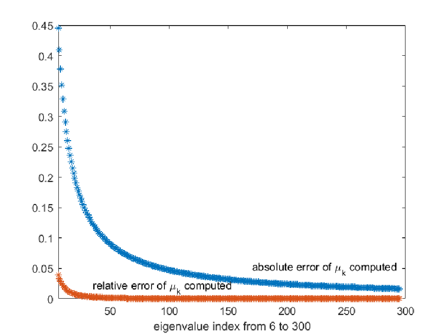
Example 1. Consider the potential (first Paine’s test, see [24]). Then (here and below we used the Matslise package [18] to compute the “exact” eigenvalues). In Fig. 1 the absolute and relative errors of computed for are presented. Here five Dirichlet-Dirichlet eigenvalues were given (), and we present the “completed” part of the Dirichlet-Dirichlet spectrum computed with (so that four coefficients in (3.10) are computed from (3.9) and together with the coefficient (3.6) they are used to compute the eigenvalues by finding zeros of the function ). It is worth mentioning that when dealing with the truncated systems of linear algebraic equations we do not seek to work with the square systems. In computations a least-squares solution of an overdetermined system (provided by Matlab, which we used in this work) gives very satisfactory results.
Of course, five eigenvalues are not enough to obtain from (2.1) a meaningful value of the parameter , so it is not clear how one could complete the spectrum in another way. Even the knowledge of ten eigenvalues still do not give the possibility to find with a reasonable accuracy. Fig. 2 shows the numbers
| (3.11) |
which according to (2.1) represent an -convergent sequence. The value of is approximately which still differs from zero considerably. The attempt to compute by minimizing the -norm of the sequence leads to a large error.

Moreover, even the knowledge of the exact value of the parameter leads to less accurate results in comparison with the spectrum completion technique based on solving the system (3.9) and finding zeros of the function . In Fig.3 we compare the absolute error of the numbers approximated by the asymptotic relation (where the exact value of is used) with the absolute error of the values of obtained with the aid of the spectrum completion technique. Even for the asymptotic approximation gives a much less accurate result than the spectrum completion technique: against .

A similar situation is observed in other examples.
Example 2. Consider the potential (second Paine’s test, see [24]). In Fig. 4 we make the same comparison: the absolute error of the numbers approximated by the asymptotic relation with the exact value of being used vs. the absolute error of the values of obtained with the aid of the spectrum completion technique.

3.2 Dirichlet-Neumann spectrum
Given several first Dirichlet-Neumann eigenvalues , let us use them to calculate the first coefficients , ,…,, where . Similarly to the case of the Dirichlet-Dirichlet spectrum, it is convenient to consider the shifted potential
That is, instead of the problem (1.1), (1.3) we consider the problem
| (3.12) |
| (3.13) |
Again the eigenfunctions do not change, and the eigenvalues are shifted:
The solution of (3.12) satisfying the initial conditions (2.5) we denote as . We have the relation
We are interested in the derivative of . It has the NSBF representation
Note that
Since zero is an eigenvalue of the problem (3.12), (3.13), we have and thus
where
Thus,
| (3.14) |
Now we complete the spectrum of the problem (3.12), (3.13) and hence also the Dirichlet-Neumann spectrum of the potential . For this we consider the equations
which can be written in the form
Taking into account (3.14), we write these equations in the form of the system of linear algebraic equations for the coefficients ,…,:
| (3.15) |
Solving this system we find ,…, as well as the parameter (from (3.14)) and the parameter .
Having computed the coefficients ,…, we consider the function
| (3.16) |
which approximates the derivative in such a way that
where is a positive constant. Theorem 3.1 is valid as well if instead of the functions and one considers the functions and . Thus zeros of approximate the Dirichlet-Neumann eigenvalues of the potential .
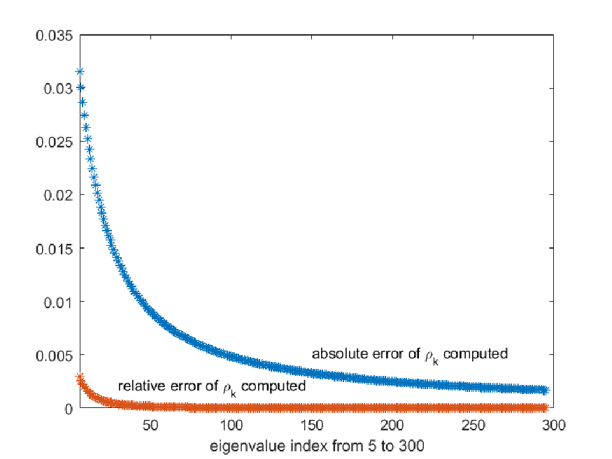
In Fig. 5 the absolute and relative errors of computed for are presented in the case of the potential from Example 2. Here five Dirichlet-Neumann eigenvalues were given (), and we present the “completed” part of the Dirichlet-Neumann spectrum computed with (so that four coefficients in (3.16) are computed from (3.15) as well as from (3.14)). The absolute error of the computed was , which is a satisfactory result taking into account the limited number of the eigenvalues given and that the relative error was approximately .
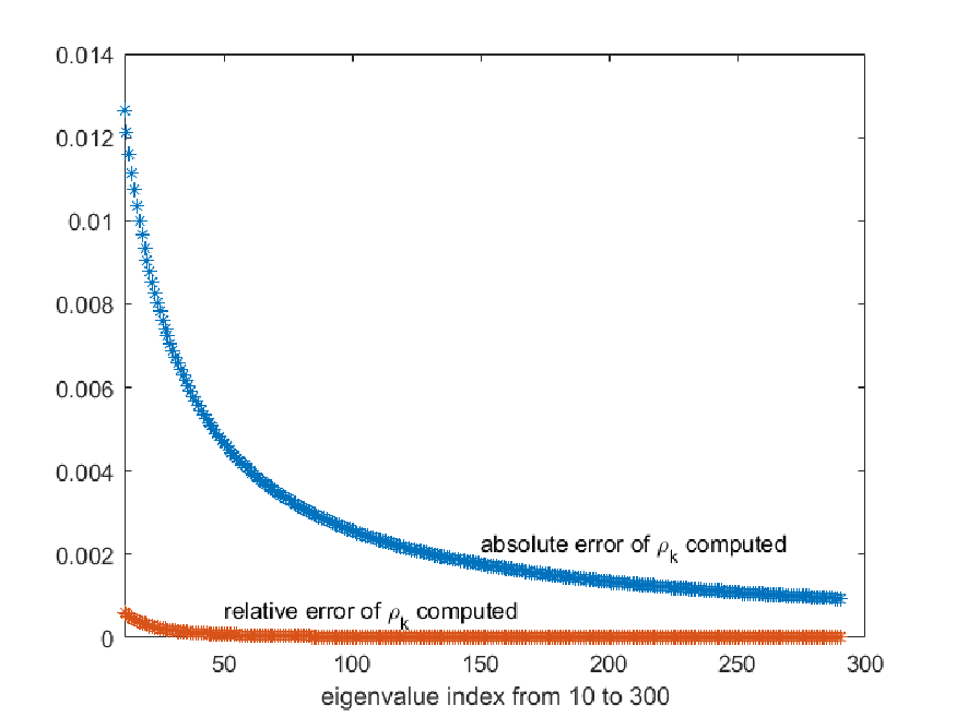
Naturally the accuracy improves when a larger number of the eigenvalues are known. In Fig. 6 the results are presented for the same potential but in the case when ten eigenvalues are known (). Here . The absolute error of the computed was already .
3.3 Completion of other spectra
Suppose several eigenvalues , ,…, of the following Sturm-Liouville problem are given
| (3.17) | ||||
| (3.18) |
where and are unknown real constants. Again, as in the previous cases, we always can shift the eigenvalues in such a way that the first shifted eigenvalue becomes zero. So, without loss of generality we assume that . Note that
and
Since zero is an eigenvalue, we have that
Thus,
| (3.19) |
where .
Now consider the characteristic function of the Sturm-Liouville problem (3.17), (3.18). Taking into account (2.6) and (2.8) it can be written in the form
Denote
Then, taking into account (3.19), we obtain
Several given eigenvalues ,…, allow us to compute several constants , , where , from the system of linear algebraic equations
Thus we obtain an approximate characteristic function of the problem (3.17), (3.18)
whose zeros approximate the square roots of the eigenvalues of the problem (3.17), (3.18).
We emphasize that to complete the spectrum of (3.17), (3.18) we require no information neither on the potential nor on the boundary conditions (the constants and remain unknown). Moreover, the parameter which appears in the second term of the asymptotics for in this problem
is computed as well, since due to (3.19), . Numerical results are similar to those for the Dirichlet-Neumann spectrum.
4 Solution of the inverse problem
Let us consider the inverse Sturm-Liouville problem consisting in recovering the potential from given several first eigenvalues of two spectra. For definiteness we restrict ourselves to the Dirichlet-Dirichlet and Dirichlet-Neumann spectra. Thus, given and , first eigenvalues of problems (1.1), (1.2) and (1.1), (1.3), respectively. In the first step, as it was explained in the previous section, we compute several coefficients , , and hence obtain the function , which approximates the characteristic function of the problem (3.1), (3.2). In the second step we compute several coefficients ,…, and then complete the spectrum of problem (1.1), (1.3). Next, let us consider the solution of equation (1.1) satisfying the initial conditions at :
Analogously to the solution (2.6) the solution admits the series representation
| (4.1) |
where are corresponding coefficients, analogous to from (2.6). Similarly to (2.12) the equality
| (4.2) |
is valid.
Note that for the solutions and are linearly dependent because both are eigenfunctions of problem (1.1), (1.3). Hence there exist such real constants , that
| (4.3) |
Moreover, these multiplier constants can be easily calculated by recalling that . Thus,
and we approximate these constants with the aid of the coefficients :
Having computed these constants we use equation (4.3) for constructing a system of linear algebraic equations for the coefficients and . Indeed, equation (4.3) can be written in the form
| (4.4) |
We have as many of such equations as many Dirichlet-Neumann singular numbers are computed. For computational purposes we choose some natural number - the number of the coefficients and to be computed. More precisely, we choose a sufficiently dense set of points and at every consider the equations
Solving this system of equations we find and and consequently and at a dense set of points of the interval . Finally, with the aid of (2.13) or (4.2) we compute .
5 Numerical examples
Consider the potential from Example 2. In Figure 7 we show the recovered potential in the case of ten pairs of the eigenvalues given. Here , the parameter was recovered with the accuracy , and additionally to the ten Dirichlet-Neumann eigenvalues given ninety eigenvalues were computed by the spectrum completion technique. Their use when constructing the system (4.4) is crucial, because the accuracy without these additional eigenvalues computed is considerably worse.

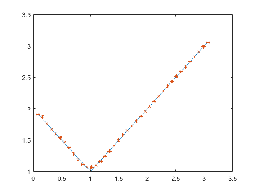
Example 3. Consider a less smooth potential
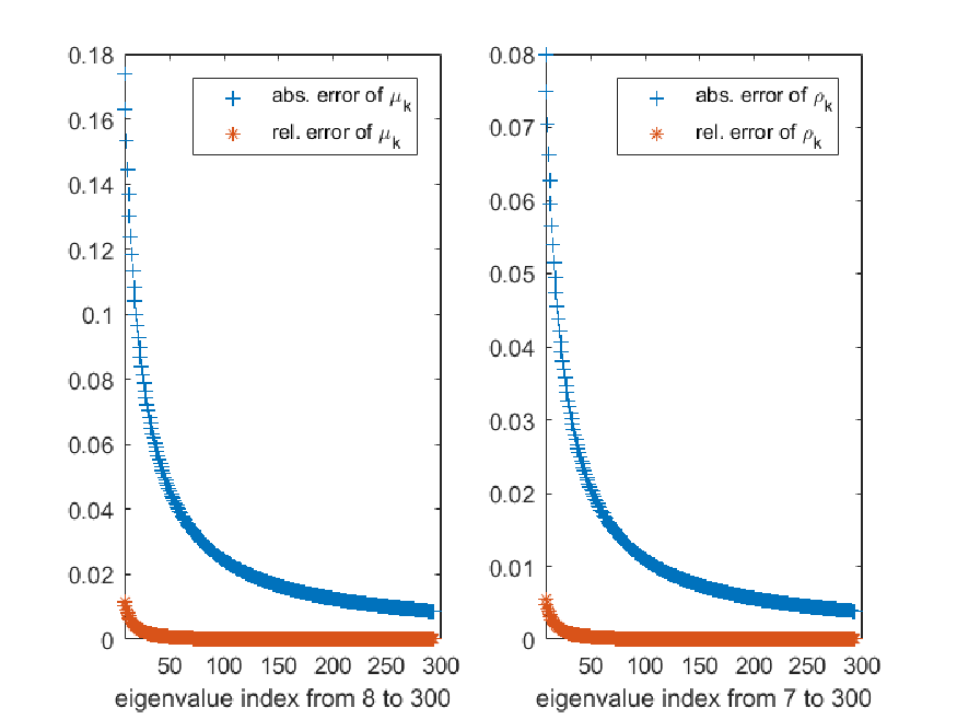
In Fig. 8 we show the results of two spectra completion in the case of seven eigenpairs given, .
The result of the recovery of the potential in this case is presented in Fig. 9.
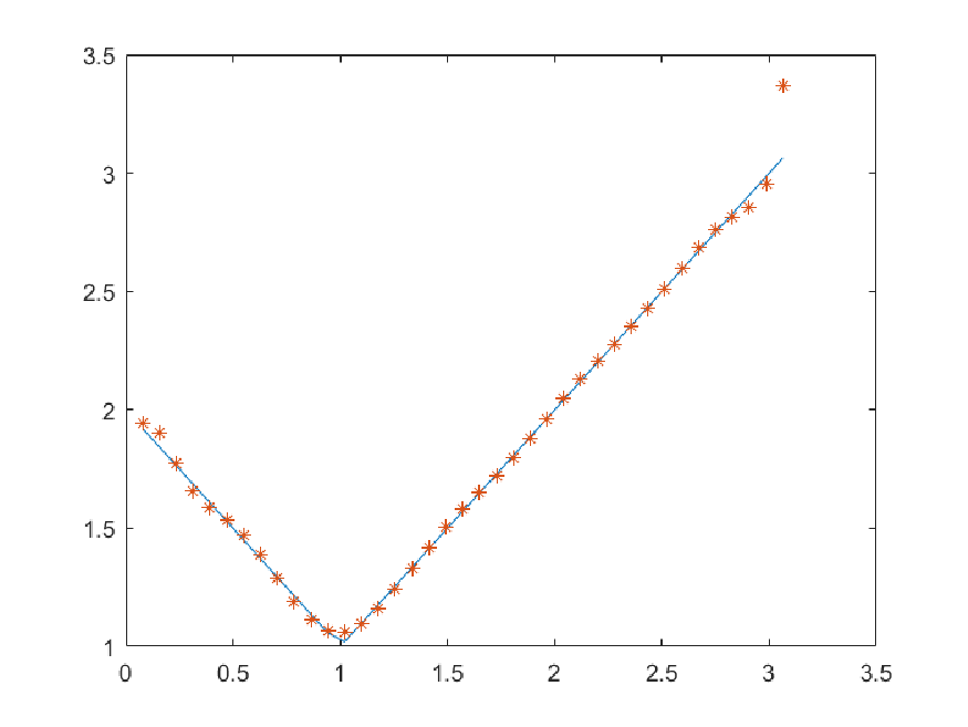
Doubling the number of the eigenpairs given (for the same number of the coefficients used, ) delivers more accurate results shown in Figs. 10 and 11.

6 Conclusions
A simple method for completing the sequence of the eigenvalues of a regular Sturm-Liouville problem is developed, which does not require neither information on the potential nor the knowledge of the boundary conditions. The spectrum is completed with a uniform absolute accuracy. Based on this spectrum completion technique a direct method for solving two-spectra inverse Sturm-Liouville problems on a finite interval is developed. The main role in the proposed approach is played by the coefficients of the Neumann series of Bessel functions expansion of solutions of the Sturm-Liouville equation and of their derivatives. The given spectral data leads to an infinite system of linear algebraic equations for the coefficients, and the potential is recovered from the first coefficient alone.
The method is simple, direct and accurate. Its performance is illustrated by numerical examples.
Acknowledgements
Research was supported by CONACYT, Mexico via the project 284470 and partially performed at the Regional mathematical center of the Southern Federal University with the support of the Ministry of Science and Higher Education of Russia, agreement 075-02-2022-893.
References
- [1] M. Abramovitz and I. A. Stegun, Handbook of mathematical functions, New York: Dover, 1972.
- [2] B. M. Brown, V. S. Samko, I. W. Knowles, M. Marletta, Inverse spectral problem for the Sturm–Liouville equation, Inverse Probl. 19 (2003), 235–252.
- [3] M.-C. Drignei, A Newton-type method for solving an inverse Sturm-Liouville problem, Inverse Probl. Sci. Eng. 23 (2015) 851–883.
- [4] Q. Gao, X. Cheng, Zh. Huang, Modified Numerov’s method for inverse Sturm–Liouville problems, J. Comput. Appl. Math. 253 (2013) 181–199.
- [5] Q. Gao, X. Cheng, Zh. Huang, On a boundary value method for computing Sturm–Liouville potentials from two spectra, Int. J. Comput. Math. 91 (2014) 490–513.
- [6] M. Ignatiev, V. Yurko, Numerical methods for solving inverse Sturm-Liouville problems, Results Math. 52 (2008), no. 1–2, 63–74.
- [7] A. Kammanee, C. Böckmann, Boundary value method for inverse Sturm-Liouville problems, Appl. Math. Comput. 214 (2009) 342–352.
- [8] A. N. Karapetyants, K. V. Khmelnytskaya, V. V. Kravchenko, A practical method for solving the inverse quantum scattering problem on a half line. Journal of Physics: Conference Series, 1540 (2020), 012007, 7pp.
- [9] V. V. Kravchenko, On a method for solving the inverse Sturm–Liouville problem, J. Inverse Ill-posed Probl. 27 (2019), 401–407.
- [10] V. V. Kravchenko, Direct and inverse Sturm-Liouville problems: A method of solution, Birkhäuser, Cham, 2020.
- [11] V. V. Kravchenko, L. J. Navarro and S. M. Torba, Representation of solutions to the one-dimensional Schrödinger equation in terms of Neumann series of Bessel functions, Appl. Math. Comput. 314 (2017), 173–192.
- [12] V. V. Kravchenko, E. L. Shishkina, S. M. Torba A transmutation operator method for solving the inverse quantum scattering problem. Inverse Problems, v. 36 (2020) 125007.
- [13] V. V. Kravchenko and S. M. Torba, Analytic approximation of transmutation operators and applications to highly accurate solution of spectral problems, Journal of Computational and Applied Mathematics 275 (2015), 1-26.
- [14] V. V. Kravchenko, S. M. Torba, A Neumann series of Bessel functions representation for solutions of Sturm-Liouville equations. Calcolo, (2018) 55: 11.
- [15] V. V. Kravchenko and S. M. Torba, A direct method for solving inverse Sturm-Liouville problems, Inverse Problems 37 (2021), 015015.
- [16] V. V. Kravchenko, S. M. Torba A practical method for recovering Sturm-Liouville problems from the Weyl function. Inverse Problems 2021, 37(6), 065011.
- [17] V. V. Kravchenko, S. M. Torba, R. Castillo-Pérez, A Neumann series of Bessel functions representation for solutions of perturbed Bessel equations. Applicable Analysis, 97, issue 5 (2018), 677–704.
- [18] V. Ledoux , M.V. Daele , G.V. Berghe , MATSLISE: a MATLAB package for the numerical solution of Sturm–Liouville and Schrödinger equations, ACM Trans. Math. Softw. 31 (2005) 532–554.
- [19] B. M. Levitan, Inverse Sturm-Liouville problems, VSP, Zeist, 1987.
- [20] B. D. Lowe, M. Pilant, W. Rundell, The recovery of potentials from finite spectral data, SIAM J. Math. Anal. 23 (1992), no. 2, 482–504.
- [21] V. A. Marchenko, Sturm-Liouville operators and applications: revised edition, AMS Chelsea Publishing, 2011.
- [22] A. Neamaty, Sh. Akbarpoor, E. Yilmaz, Solving inverse Sturm-Liouville problem with separated boundary conditions by using two different input data, Int. J. Comput. Math. 95 (2018), 1992–2010.
- [23] A. Neamaty, Sh. Akbarpoor, E. Yilmaz, Solving symmetric inverse Sturm–Liouville problem using Chebyshev polynomials, Mediterr. J. Math. (2019) 16:74.
- [24] J. D. Pryce, Numerical solution of Sturm-Liouville problems, Clarendon Press, Oxford, 1993.
- [25] N. Röhrl, A least squares functional for solving inverse Sturm-Liouville problems, Inverse Probl. 21 (2005), 2009–2017.
- [26] W. Rundell, P. E. Sacks, Reconstruction techniques for classical inverse Sturm–Liouville problems, Math. Comput. 58 (1992), 161–183.
- [27] P. E. Sacks, An iterative method for the inverse Dirichlet problem, Inverse Probl. 4 (1988), 1055-1069.
- [28] E. L. Shishkina and S. M. Sitnik, Transmutations, singular and fractional differential equations with applications to mathematical physics, Elsevier, Amsterdam, 2020.
- [29] V. A. Yurko, Introduction to the theory of inverse spectral problems, Fizmatlit, Moscow, 2007 (in Russian).