Superconducting microsphere magnetically levitated in an anharmonic potential with integrated magnetic readout
Abstract
Magnetically levitated superconducting microparticles offer a promising path to quantum experiments with picogram to microgram objects. In this work, we levitate a superconducting microsphere in a magnetic chip trap in which detection is integrated. We measure the particle’s center-of-mass motion using a DC-SQUID magnetometer. The trap frequencies are continuously tunable between 30 and and the particle remains stably trapped over days in a dilution refrigerator environment. We characterize motional-amplitude-dependent frequency shifts, which arise from trap anharmonicities, namely Duffing nonlinearities and mode couplings. We explain this nonlinear behavior using finite element modelling of the chip-based trap potential. This work constitutes a first step towards quantum experiments and ultrasensitive inertial sensors with magnetically levitated superconducting microparticles.
I Introduction
Systems of levitated nano- and microparticles in vacuum Ashkin and Dziedzic 1976 offer extreme isolation of the particles from the environment as well as in-situ tuning of the trapping potential Millen et al. 2020; Gonzalez-Ballestero et al. 2021. These platforms provide novel opportunities for realizing ultrasensitive force Ranjit et al. 2016; Prat-Camps et al. 2017; Monteiro et al. 2020; Weiss et al. 2021 and acceleration sensors Goodkind 1999; Moody et al. 2002; Johnsson et al. 2016; Monteiro et al. 2017; Timberlake et al. 2019, for studying thermodynamics in the underdamped regime Li et al. 2010; Gieseler and Millen 2018; Debiossac et al. 2020, for exploring many-body physics with massive objects Dholakia and Zemánek 2010; Lechner et al. 2013; Simpson et al. 2016; Yan et al. 2022; Rieser et al. 2022, and for exploiting rotational degrees of freedom Delord et al. 2017; Perdriat et al. 2021; Stickler et al. 2021; Rusconi et al. 2022. Recently, the center-of-mass (COM) motion of optically levitated nanospheres was cooled to the motional ground state Delić et al. 2020; Magrini et al. 2021; Tebbenjohanns et al. 2021; Ranfagni et al. 2022; Piotrowski et al. 2023, opening the possibility to perform quantum experiments with levitated nanoparticles Romero-Isart et al. 2011; Romero-Isart 2011; Gonzalez-Ballestero et al. 2021. Electrically levitated nanoparticles have also seen tremendous progress towards reaching the quantum regime Fonseca et al. 2016; Goldwater et al. 2019; Martinetz et al. 2020; Perdriat et al. 2021; Dania et al. 2021.
To extend quantum control from nano- to microparticles, magnetic levitation Moon and Chang 1994 has recently gained renewed interest Takahashi et al. 2017; Timberlake et al. 2019; Vinante et al. 2020; Zheng et al. 2020a; Leng et al. 2021; Brown et al. 2021; Arrayás et al. 2021; Hofer et al. 2022; Latorre et al. 2022. Magnetic levitation can be used to levitate objects of different shapes Latorre et al. 2020; Navau et al. 2021 with masses ranging from picograms to tons Moon and Chang 1994. It offers extreme isolation from the environment Romero-Isart et al. 2012; Cirio et al. 2012; Vinante et al. 2020; Zheng et al. 2020a; Leng et al. 2021; Hofer et al. 2022 and allows for tunable potential landscapes Pino et al. 2018. This combination of properties makes magnetically levitated particles particularly well suited for high precision sensing of forces and accelerations Goodkind 1999; Moody et al. 2002; Johnsson et al. 2016; Jackson Kimball et al. 2016; Prat-Camps et al. 2017; Timberlake et al. 2019, as well as for fundamental physics experiments with picogram to microgram objects Romero-Isart et al. 2012; Cirio et al. 2012; Pino et al. 2018. Recent experimental developments in this direction include levitating micro-magnets on top of superconductors Niemetz et al. 2000; Wang et al. 2019; Timberlake et al. 2019; Vinante et al. 2020; Gieseler et al. 2020, diamagnetic particles in strong magnetic fields Takahashi et al. 2017; Slezak et al. 2018; Zheng et al. 2020a; Leng et al. 2021; Brown et al. 2021, and superconducting microparticles in millimeter-scale superconducting magnetic traps van Waarde 2016; Latorre et al. 2022; Hofer et al. 2022.
We pursue magnetic levitation of superconductors in a superconducting magnetic trap, since this approach promises the least intrinsic mechanical dissipation Romero-Isart et al. 2012; Cirio et al. 2012. Levitated superconductors in the Meissner state do not suffer from magnetic moment drift or intrinsic eddy current damping, unlike levitated magnets Prat-Camps et al. 2017; Timberlake et al. 2019; Wang et al. 2019; Vinante et al. 2020; Gieseler et al. 2020. By using a persistent current magnetic trap van Waarde et al. 2016 the trap can be made perfectly stable, unlike systems of diamagnetic particles levitated between strong magnets Hsu et al. 2016; Slezak et al. 2018; Zheng et al. 2020a.
We levitate a superconducting microsphere in a fully chip-based system. The chip-based approach Weinstein and Libbrecht 1995; Reichel et al. 1999; Latorre et al. 2022 enables higher magnetic field gradients and trapping frequencies, as well as the potential to scale up the system to levitate multiple particles on the same chip. We measure the particle’s motion using magnetic pickup loops which are coupled to a SQUID magnetometer. The pickup loops are integrated in the chip; this allows for precise positioning and enhanced measurement sensitivity. In the future we will replace the SQUID by a flux-tunable superconducting microwave cavity Rodrigues et al. 2019; Zoepfl et al. 2020; Schmidt et al. 2020; Bera et al. 2021; Luschmann et al. 2022; Zoepfl et al. 2023 to achieve quantum control over the COM motion of the levitated microparticle Romero-Isart et al. 2012; Cirio et al. 2012; Johnsson et al. 2016; Pino et al. 2018.
In this work we demonstrate stable levitation of a -diameter () superconducting microsphere over days. We smoothly tune the particle’s COM frequencies between 30 and by varying the trap current. We observe that the COM frequencies depend on the motional amplitudes. This arises from trap anharmonicities Gieseler et al. 2013; Gieseler et al. 2014; Fonseca et al. 2016; Setter et al. 2019; Zheng et al. 2020b; Flajšmanová et al. 2020. The observed behavior is consistent with estimations of the trap anharmonicities extracted from finite element modelling (FEM) of our system. In the future we will employ cryogenic vibration isolation Maisonobe et al. 2018; Wit et al. 2019 and feedback cooling Rossi et al. 2018; Magrini et al. 2021; Tebbenjohanns et al. 2021 to reduce the motional amplitudes, then the effects of trap anharmonicities will be mitigated.
II Experimental setup
The magnetic trap is produced by a current flowing in two superconducting coils, which are patterned on two silicon chips. The chips are stacked on top of each other to form an anti-Helmholtz-like configuration (see Fig. 1), for details see Ref. Latorre et al. 2022. The superconducting particle stably levitates near the minimum of the trap’s magnetic field. The particle is confined within a closed container given by the side walls of the hole in the top chip, the top surface of the bottom chip, and a glass slide on top of the hole. The force due to the magnetic trapping field is restoring within the container’s bounds, with a trap depth larger than . To detect the particle motion, we use two pickup loops which are integrated on the same chips, see Fig. 1.
As the particle moves it changes the magnetic flux threading the pickup loops and thus the current induced in the loops. The pickup loops are connected to a commercial DC-SQUID magnetometer, which transduces the flux into a measurable voltage. Typical pickup efficiencies are for the three COM modes, in terms of the flux coupled into the SQUID, and where is the magnetic flux quantum. due to the system’s geometry (see Appendix S2). The measurement noise floor () is limited by magnetic field fluctuations caused by trap current fluctuations and corresponds to a noise floor of for displacements along the directions, respectively. We connect the pickup loops in series to reduce the sensitivity to these field fluctuations. In the future, we will mitigate this noise by driving the trap using a persistent current van Waarde et al. 2016, which should enable reaching the intrinsic noise floor of the SQUID ().
The magnetic trap and the SQUID magnetometer are thermally connected to the mixing stage of a dilution refrigerator. This allows the experiment to operate between temperatures as low as and as high as the critical temperature of the superconducting particle ( for lead). Before levitating, the particle thermalizes on the bottom chip surface to the temperature of the chip substrate [see Fig. 1(b)]. To lift the particle off the chip surface, we ramp the trap current up to to overcome the adhesive force between the particle and the chip surface. With a current of , the lift force is , which is usually sufficient to lift the particle. After that, the current is ramped down to the operating trap current.
III Characterization of center-of-mass motion
Near the trap center, the particle experiences a harmonic trapping potential. The COM frequencies depend on the trap geometry, the particle’s density, and the trap current. The penetration depth ( for lead) is much smaller than the particle radius () and so the particle can be modelled as an ideal diamagnet with magnetic susceptibility of and its trapping frequencies are given by Hofer and Aspelmeyer 2019
| (1) |
where is the magnetic field gradient along the direction at the trap center, is the vacuum permeability, is the trap current, is the number of trap coil windings, is the trap coil inner radius, is the particle’s density and is a geometric factor. At the center of an ideal anti-Helmholtz configuration . In our system , and . (our coils are separated by and have inner radii as shown in Appendix S2). The trap axes are indicated in Fig. 1(a).
Fig. 2(a) shows the power spectrum of a levitated microsphere. Throughout this work, unless otherwise stated, we levitated a -diameter lead sphere using trap current and the cryostat temperature was . The peaks corresponding to the COM motion are colored.
We identified these modes by comparing the peak frequencies with predictions from FEM simulations of our system Latorre et al. 2020; Latorre et al. 2022. We find good agreement between the measured and simulated COM frequencies. Peaks at the second harmonic of the COM frequencies are pronounced, particularly the second harmonic of the peak at . These peaks arise from the nonlinear pickup efficiency, rather than due to actual particle motion at these frequencies. We describe these peaks further in Appendix S3. In the future we will feedback cool the particle, then effects of the nonlinear pickup will be negligible.
The linear relation between the COM frequencies and the trap current given by Eq. 1 is shown in Fig. 2(b). We observed no significant difference between measuring this effect with the cryostat temperature of or . We find good agreement between measurement results and FEM simulation results for the and modes. We attribute the discrepancy for the -mode frequency to simulation uncertainties in the FEM.
We confirm the inverse relation between trapping frequency and particle density of Eq. 1 by comparing the trapping frequencies of a lead particle and a tin-lead particle as we vary the trap current, see Fig. 2(c). The ratio of the frequencies is given by the square root of the ratio of the material densities.
We can stably levitate the superconducting sphere for days in the chip-based magnetic trap. Fig. 3(a) shows the fluctuations of the COM frequencies of a levitated sphere over a 35 h measurement. We have yet to observe an upper limit to the levitation time, provided that the particle is not illuminated. When the particle is illuminated, as in Ref. Latorre et al. 2022, it heats up, loses superconductivity and falls on the bottom chip. When the particle is kept in the dark, as in this work, we have not yet observed any upper limit to the levitation time; we have measured up to 48 h.
Around once per day, we observe a sudden jump of all the COM frequencies of around (see Appendix S5). We attribute these jumps to changes in the magnitude or orientation of trapped flux in the particle. Fig. 3(a) shows 35 h of data in which we do not discern any such frequency jumps. The trapped flux will be the topic of a dedicated future investigation.
The particle’s COM motion does not thermalize at the cryostat temperature, since it is strongly driven by the cryostat’s vibrations. We estimate the mean amplitudes of the three modes to be , , and for the x, y, and z modes, respectively, corresponding to an effective temperature of about . The energy in each mode () fluctuates on a time scale , as shown by the autocorrelation functions in Fig. 3(b). The mode energy fluctuations are due to the mode amplitude fluctuations, which occur over this time scale. By fitting the autocorrelation functions to exponential decay functions, we extract quality factors 3400, 4500, and 9300 for the x, y, and z modes, respectively Zheng et al. 2020a. We expect the quality factors to be limited by eddy current damping caused by normal-conducting metals in the vicinity of the levitated particle. In the future, we will mitigate this damping mechanism by surrounding the particle with a superconducting shield, with no normal-conducting metal within the shield.
IV Frequency pulling
We can explain the COM frequency fluctuations of Fig. 3(a) as resulting from the fluctuating mode amplitudes [Fig. 3(b)] together with frequency pulling. Frequency pulling describes the dependence of the COM frequencies on the mode amplitudes. It arises from quartic terms in the trapping potential of the form
| (2) |
which cause the motional frequencies to be shifted depending on the motional amplitudes according to Bachtold et al. 2022
| (3) |
The terms in the potential are called Duffing nonlinearities, while the terms describe couplings between the modes.
Experimental data showing frequency pulling is shown in Fig. 4. The spectral peak corresponding to the x-mode (y-mode) shifts depending on the amplitude of the x-mode motion in Fig. 4(a) [(b)]. This is described by Eq. 3. The remaining seven graphs showing the dependence of on are included in Appendix S4.
The linear relation between the mode frequencies and the mean-square displacements [Eq. 3] are shown in Fig. 4(c) and (d), in which the spectral peak frequencies and are plotted against the spectral peak area corresponding to the x-mode (the remaining graphs of the same form are included in Appendix S4). The slopes of these lines depend on the values of and as well as the pickup efficiency . We extract estimates of from FEM simulations of our system (see Appendix S1); this allows us to use the nine gradients (i.e. the nine linear relations between and , for and ) to estimate the three efficiencies (the values are quoted earlier). The estimated efficiencies are used to convert the lower x-axes of Fig. 4(c)-(d) into the upper x-axes, and yield the secondary y-axis of Fig. 2(a).
The estimation of the three efficiencies is an over-constrained problem, it yields fairly consistent results for the nine graphs. For instance, the estimation of together with the FEM estimations of and describes well both the slope in Fig. 4(c) and Fig. 4(d).
To observe the frequency pulling effect presented in Fig. 4 we did not control the particle’s motional amplitudes, instead, we filtered a long 35 h dataset in which the motional amplitudes randomly fluctuated: We separated the data into 10 s chunks and extracted the mode frequencies and mode areas from each chunk.
To investigate the dependence of the mode frequencies on, e.g., the x-mode amplitude, we filtered out the data in which the y- and z-mode amplitudes were high. Each point in Fig. 4(c)-(d) corresponds to one 10 s chunk. To produce the seven spectra in Fig. 4(a) and (b) we binned the power spectrum of each 10 s-long dataset into seven bins, based on the x-peak areas, then we averaged the power spectra for each of the seven bins.
The mode amplitude fluctuations together with frequency pulling describe the frequency fluctuations of Fig. 3(a). We represent the frequency distributions by histograms in Fig. 4(e)-(g); we note they are asymmetric. We also plot histograms based on the frequency pulling model; the model histograms were constructed by predicting the mode frequencies for each 10 s interval of data based on the measured mode amplitudes, the nonlinear coefficients and the pickup efficiencies . The model histograms describe the observed frequency fluctuations well.
Because the modes are coupled via the trap anharmonicity [Eq. 3] we expect the average energies of the modes to be similar. We can estimate the mean energies of the modes using the estimated pickup efficiencies , and we find . Because the estimated average energies rely on the estimated pickup efficiencies, the similarity of the average energies lends credence to our estimates of .
V Conclusions
In conclusion, we have demonstrated an integrated superconducting chip device for magnetic levitation and detection of superconducting microparticles at mK temperatures. We have shown a good understanding of the trap potential, the COM motion, and inductive coupling by comparing trap models with measurements. Further, we have demonstrated that the COM frequencies can be tuned via the trap current and that the system is stable over days. For the large motional amplitudes in our experiments, we observe nonlinear behavior and mode coupling of the COM particle motion, in the form of amplitude-dependent frequency shifts.
Future experiments will employ a cryogenic passive vibration isolation system Maisonobe et al. 2018; Wit et al. 2019, which will decouple the particle motion from external mechanical vibrations. Such vibration isolation systems can attenuate our measured mechanical vibrations of about by more than six orders of magnitude to achieve thermally driven COM motion at . Further, the detection noise floor can be greatly reduced by the use of a persistent current trap van Waarde et al. 2016 and improved magnetic shielding, which should allow us to reach the intrinsic noise floor of of our commercial SQUID. Alternatively, the particle motion can also be measured using flux-sensitive superconducting microwave resonators Rodrigues et al. 2019; Zoepfl et al. 2020; Schmidt et al. 2020; Luschmann et al. 2022; Zoepfl et al. 2023. Furthermore, the pick-up efficiency can be increased by placing the pick-up coil closer to the particle, by using multi-winding coils, and by improving the flux-transfer efficiency to the SQUID. We estimate that these measures will yield an improvement in the pick-up efficiency of four orders of magnitude. This improvement is enabled by our understanding of the chip-based particle motion detection and the flexibility in the microfabrication of pick-up loops of our chip-based approach. Overall, the reduction of technical noise and increase in pick-up efficiency should enable feedback cooling to the quantum ground state Rossi et al. 2018; Magrini et al. 2021; Tebbenjohanns et al. 2021 of the COM motion of microparticles, which would serve as a gateway to generating quantum states of nano- to microgram masses Romero-Isart et al. 2012; Cirio et al. 2012; Johnsson et al. 2016.
The data of this study are openly available in zenodo.org at https://doi.org/10.5281/zenodo.7304535.
Acknowledgements.
We gratefully acknowledge Axel Eriksson, Andreas Isacsson, Philip Schmidt, Joachim Hofer, and Fabian Resare for insightful discussions and Joachim Hofer also for sharing of code. This work was supported in part by the Horizon Europe 2021-2027 Framework Programme under the Grant Agreement number 101080143 (SuperMeQ), the QuantERA project C’MON-QSENS!, the Knut and Alice Wallenberg Foundation through a Wallenberg Academy Fellowship (W.W.), by the Wallenberg Center for Quantum Technology (WACQT, A.P.), by Chalmers Excellence Initiative Nano, and by the Swedish Research Council (Grant 2020-00381, G.H.). Sample fabrication was performed in the Myfab Nanofabrication Laboratory at Chalmers. Simulations were performed on resources provided by the Swedish National Infrastructure for Computing (SNIC) at Tetralith, Linköping University, partially funded by the Swedish Research Council (Grant 2018-05973).Supplemental Material
S1 Extracting the trap anharmonicity from FEM
We consider anharmonicities in the trapping potential up to quartic terms. The potential can then be described as
| (S1) | ||||
The force acting on the particle is
| (S2) |
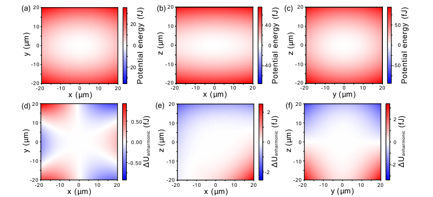
The FEM simulations give us the force acting on the particle due to the trapping potential at different displacements, as described in Ref. Latorre et al. 2020. We fit the FEM results by Eq. S2 with the coefficients of the trapping potential of Eq. S1 as free parameters. In this way we extract the trapping potential coefficients from the FEM simulations.
Note, in comparing with from the main text:
| (S3) | ||||
The potential energy which we calculate based on fitting the FEM simulations is represented in Fig. S1. We calculate the potential energy in 3D; in the figure 2D slices are shown. Fig. S1 also shows the relative contribution of the cubic and quartic terms to the potential.

S2 Measurement of particle motion
As the particle displacement oscillates the magnetic flux threading the pickup loops oscillates in response. This oscillating flux of the pickup loops is transferred to the SQUID loop. The flux at the SQUID loop is converted into a voltage signal. In this section each of these steps are described in turn.
S2.1 Inductive coupling to particle motion
We estimate the response of the change of flux threading the pickup loops in response to displacement of the particle along x, y and z by treating the trapping field as a magnetic quadrupole field (which is a good approximation near the center), using Eq. (5) from Hofer and Aspelmeyer 2019, and using knowledge of the geometry of our system (represented in Fig. S3).

The results are shown in Fig. S4. The response to displacement along all directions is nonlinear. That is to say, the response has strong quadratic components () which we describe by the parameter in Section S3.2. We note that the response of the pickup to displacement along the z direction is largely linear, whereas the response to x and y displacements has a clear quadratic component. The response can be made more linear along the x and y directions by changing the geometry such that the particle equilibrium position is displaced further from the center of the pickup loops. Because the pickup loops are connected in series, the overall pickup-loop flux is the sum of the fluxes in each loop.
S2.2 Flux transfer from the pickup loops to the SQUID loop
Fig. S5 shows how the pickup loops are electrically connected to the SQUID via an input coil. The flux transfer is given by
| (S4) |
where is the input coil inductance, is the parasitic inductance which is dominated by the inductance of the twisted wire pairs, is the pickup inductance, and is the mutual inductance between the SQUID loop and the input coil inductance. Using these values, we estimate the flux transfer efficiency . By improving the inductance matching, can be improved to 0.5.
Based on the dependence of the pickup-loop flux on the particle displacement (Fig. S4) and the flux transfer efficiency from the pickup loops to the SQUID loop Eq. S4 we make independent estimates of the pickup efficiency in the pick-up loop . These values are close to the ones found by using the measurement data and the model for the potential energy, where we obtain . We note that we obtain the latter values by dividing the pickup efficiencies in terms of flux in the SQUID by the flux transfer efficiency , i.e., . The small discrepancy may arise because our estimates of the response of the pickup loops to displacements along and using the data in Fig. S4 depend critically on our knowledge of the particle’s equilibrium position, due to the nonlinearity of the pickup efficiency. Additionally, we made the simplifying assumption in Section S2.1 of a magnetic quadrupole field at the trap center.
S2.3 Flux in SQUID loop converted to SQUID voltage
We operate the SQUID in flux-locked loop mode. Then the SQUID output voltage is related to the SQUID loop flux by
| (S5) |
where is the mutual inductance between the feedback electronics and the SQUID, and describes the resistor used in the feedback electronics.
S3 Harmonics in spectra
As well as observing the peaks in the spectra at frequencies , and corresponding to COM motion along the x, y and z directions, we observe strong peaks at frequencies , and (see the power spectrum in Fig. S6).
We observe that the peak areas of the second-harmonic peaks grow quadratically with the peak areas of the respective fundamental peaks, as shown in Fig. S2. The fundamental and harmonic peak areas and are related by
| (S6) |
The factor describes the observed quadratic relation between the peak areas, it is different for each mode. From the data in Fig. S2 we extract for x, y and z modes, respectively (in this section we work with the spectral peak areas in units of , that is why has units ).
Constructing Fig. S2 involved breaking the 35 h-long dataset which was used in Fig. 3 and Fig. 4 of the main text into 10 s chunks, we then calculated the power spectrum for each 10 s chunk and extracted the peak areas for the three fundamental and three second harmonic peaks and compared them.
Below, we estimate that the actual motion of the particle at frequencies , and arising from the trap anharmonicity is negligible. Instead, we believe the second harmonics arise primarily due to the pickup nonlinearity.
S3.1 Particle motion at the second harmonic frequency arising from the trap anharmonicity
In a potential of the form
| (S7) |
the particle will move with a component at frequency and a component at frequency . The amplitudes of these motions, at the fundamental frequency and at the harmonic frequency, are related by
| (S8) |
provided that the cubic term in the potential is a perturbation and provided that the motional amplitudes are small.
We derive this equation by solving the equation of motion in this potential looking for a solution of the form
| (S9) |
in the regime when .
Because the peak areas are related to the mean-square amplitudes by we expect the nonlinearity of the trapping potential to give
| (S10) |
And thus, using the values extracted from FEM (see Section S1) we expect for the x, y and z modes. These values are much smaller than the observed values , and so the second harmonic peaks do not arise from motion of the particle at the second harmonic frequencies.
S3.2 Second harmonic peaks caused by the pickup nonlinearity
A particle in a 1D harmonic potential moves according to
| (S11) |
As described in Section S2.1 and Fig. S4, the flux threading the pickup loops depends nonlinearly on the particle position . This can be captured by the quadratic function
| (S12) | ||||
| (S13) |
Here and are conversion factors from particle displacement to pickup-loop flux; describes the linear response of the pickup-loop, while describes the quadratic response. is an offset.
The SQUID voltage signal is related to the flux threading the pickup loops by
| (S14) |
where we define the conversion factor . And so, the voltage signal is related to the particle position by
| (S15) | ||||
| (S16) |
where and are conversion factors from particle displacement to SQUID voltage; describes the linear response of the SQUID, while describes the quadratic response, is an offset. We see that
| (S17) |
In the power spectrum of the voltage signal, the area of the fundamental peak is and the area of the harmonic peak is . And so
| (S18) |
and
| (S19) |
Earlier we defined
| (S20) |
So, we identify
| (S21) |
Overall, the nonlinearity of the pickup should give
| (S22) |
We extract and for the different directions , and using the data in Fig. S4, and we extract from the comparison of the observed frequency pulling (see Section S4) with the trap anharmonicities given by FEM (see Section S1). And so, we estimate . These are order-of-magnitude estimations, since the estimations of depend critically on our estimation of the position of the trap center. The estimates are similar in magnitude to the observed values of for the x and y modes, and so we believe the spectral peaks at the second harmonics arise from the nonlinear pickup.
S4 Frequency pulling
Figures Fig. S7 and Fig. S8 employ the same dataset and analysis method as was used to construct Fig. 4(a-d) of the main text. While Fig. 4(a-d) shows the dependence of and on , Fig. S8 and Fig. S7 show the dependence of , and on , and .
In Fig. S7 the blue-colored straight lines represent linear fits to the data, they are meant as guides to the eye. The model curves are given by Eq. (3) in the main text. We extract estimates of the values from FEM (details in Section S1). In Fig. S8(a-i) the x-axes are the mean-square displacements in units of , and thus the gradients of the nine model lines depend on the three pickup efficiencies [In (a-c) the gradients depend on , (d-f) depend on and (g-i) depend on ]. We treat the three pickup efficiencies as free parameters, and we obtain three estimates for each , from the data in each of the panels. We choose the values which provide the best agreement between the observations and the model. In this way we use the frequency pulling data to estimate the pickup efficiencies .

S5 Frequency jumps
When we levitate a particle we occasionally observe sudden changes of all the COM frequencies at once. These changes appear to happen at random times. We expect these frequency jumps are due to reorientation of trapped flux in the particle, or due to a change of the amount of the trapped flux in the particle. In Fig. S9 three such frequency jumps are indicated by arrows. Here the particle was levitated for two days. The 35 h dataset used in Fig. 3 and Fig. 4 used the data between time 4 h and 39 h of this dataset.

References
- Ashkin and Dziedzic (1976) A. Ashkin and J. M. Dziedzic, Optical levitation in high vacuum, Appl. Phys. Lett. 28, 333 (1976).
- Millen et al. (2020) J. Millen, T. S. Monteiro, R. Pettit, and A. N. Vamivakas, Optomechanics with levitated particles, Rep. Prog. Phys. 83, 026401 (2020).
- Gonzalez-Ballestero et al. (2021) C. Gonzalez-Ballestero, M. Aspelmeyer, L. Novotny, R. Quidant, and O. Romero-Isart, Levitodynamics: Levitation and control of microscopic objects in vacuum, Science 374, 3027 (2021).
- Ranjit et al. (2016) G. Ranjit, M. Cunningham, K. Casey, and A. A. Geraci, Zeptonewton force sensing with nanospheres in an optical lattice, Phys. Rev. A 93, 053801 (2016).
- Prat-Camps et al. (2017) J. Prat-Camps, C. Teo, C. C. Rusconi, W. Wieczorek, and O. Romero-Isart, Ultrasensitive inertial and force sensors with diamagnetically levitated magnets, Phys. Rev. Appl. 8, 034002 (2017).
- Monteiro et al. (2020) F. Monteiro, W. Li, G. Afek, C.-l. Li, M. Mossman, and D. C. Moore, Force and Acceleration Sensing with Optically Levitated Nanogram Masses at Microkelvin Temperatures, Phys. Rev. A 101, 053835 (2020).
- Weiss et al. (2021) T. Weiss, M. Roda-Llordes, E. Torrontegui, M. Aspelmeyer, and O. Romero-Isart, Large quantum delocalization of a levitated nanoparticle using optimal control: Applications for force sensing and entangling via weak forces, Phys. Rev. Lett. 127, 023601 (2021).
- Goodkind (1999) J. M. Goodkind, The superconducting gravimeter, Rev. Sci. Instrum. 70, 4131 (1999).
- Moody et al. (2002) M. V. Moody, H. J. Paik, and E. R. Canavan, Three-axis superconducting gravity gradiometer for sensitive gravity experiments, Rev. Sci. Instrum. 73, 3957 (2002).
- Johnsson et al. (2016) M. T. Johnsson, G. K. Brennen, and J. Twamley, Macroscopic superpositions and gravimetry with quantum magnetomechanics, Sci. Rep. 6, 37495 (2016).
- Monteiro et al. (2017) F. Monteiro, S. Ghosh, A. G. Fine, and D. C. Moore, Optical levitation of 10-ng spheres with nano-g acceleration sensitivity, Phys. Rev. A 96, 063841 (2017).
- Timberlake et al. (2019) C. Timberlake, G. Gasbarri, A. Vinante, A. Setter, and H. Ulbricht, Acceleration sensing with magnetically levitated oscillators above a superconductor, Appl. Phys. Lett. 115, 224101 (2019).
- Li et al. (2010) T. Li, S. Kheifets, D. Medellin, and M. G. Raizen, Measurement of the instantaneous velocity of a brownian particle, Science 328, 1673 (2010).
- Gieseler and Millen (2018) J. Gieseler and J. Millen, Levitated Nanoparticles for Microscopic Thermodynamics—A Review, Entropy 20, 326 (2018).
- Debiossac et al. (2020) M. Debiossac, D. Grass, J. J. Alonso, E. Lutz, and N. Kiesel, Thermodynamics of continuous non-Markovian feedback control, Nat. Commun. 11, 1360 (2020).
- Dholakia and Zemánek (2010) K. Dholakia and P. Zemánek, Colloquium: Gripped by light: Optical binding, Rev. Mod. Phys. 82, 1767 (2010).
- Lechner et al. (2013) W. Lechner, S. J. M. Habraken, N. Kiesel, M. Aspelmeyer, and P. Zoller, Cavity optomechanics of levitated nanodumbbells: Nonequilibrium phases and self-assembly, Phys. Rev. Lett. 110, 143604 (2013).
- Simpson et al. (2016) S. H. Simpson, L. Chvátal, and P. Zemánek, Synchronization of colloidal rotors through angular optical binding, Phys. Rev. A 93, 023842 (2016).
- Yan et al. (2022) J. Yan, X. Yu, Z. V. Han, T. Li, and J. Zhang, On-demand assembly of optically-levitated nanoparticle arrays in vacuum (2022), arXiv:2207.03641 .
- Rieser et al. (2022) J. Rieser, M. A. Ciampini, H. Rudolph, N. Kiesel, K. Hornberger, B. A. Stickler, M. Aspelmeyer, and U. Delić, Tunable light-induced dipole-dipole interaction between optically levitated nanoparticles, Science 377, 987 (2022).
- Delord et al. (2017) T. Delord, L. Nicolas, L. Schwab, and G. Hétet, Electron spin resonance from nv centers in diamonds levitating in an ion trap, New J. Phys. 19, 033031 (2017).
- Perdriat et al. (2021) M. Perdriat, C. Pellet-Mary, P. Huillery, L. Rondin, and G. Hétet, Spin-mechanics with nitrogen-vacancy centers and trapped particles, Micromachines 12, 651 (2021).
- Stickler et al. (2021) B. A. Stickler, K. Hornberger, and M. S. Kim, Quantum rotations of nanoparticles, Nat. Rev. Phys. 3, 589 (2021).
- Rusconi et al. (2022) C. C. Rusconi, M. Perdriat, G. Hétet, O. Romero-Isart, and B. A. Stickler, Spin-controlled quantum interference of levitated nanorotors, Phys. Rev. Lett. 129, 093605 (2022).
- Delić et al. (2020) U. Delić, M. Reisenbauer, K. Dare, D. Grass, V. Vuletić, N. Kiesel, and M. Aspelmeyer, Cooling of a levitated nanoparticle to the motional quantum ground state, Science 367, 892 (2020).
- Magrini et al. (2021) L. Magrini, P. Rosenzweig, C. Bach, A. Deutschmann-Olek, S. G. Hofer, S. Hong, N. Kiesel, A. Kugi, and M. Aspelmeyer, Real-time optimal quantum control of mechanical motion at room temperature, Nature 595, 373 (2021).
- Tebbenjohanns et al. (2021) F. Tebbenjohanns, M. L. Mattana, M. Rossi, M. Frimmer, and L. Novotny, Quantum control of a nanoparticle optically levitated in cryogenic free space, Nature 595, 378 (2021).
- Ranfagni et al. (2022) A. Ranfagni, K. Børkje, F. Marino, and F. Marin, Two-dimensional quantum motion of a levitated nanosphere, Phys. Rev. Research 4, 033051 (2022).
- Piotrowski et al. (2023) J. Piotrowski, D. Windey, J. Vijayan, C. Gonzalez-Ballestero, A. de los Ríos Sommer, N. Meyer, R. Quidant, O. Romero-Isart, R. Reimann, and L. Novotny, Simultaneous ground-state cooling of two mechanical modes of a levitated nanoparticle, Nat. Phys. , 1 (2023).
- Romero-Isart et al. (2011) O. Romero-Isart, A. C. Pflanzer, F. Blaser, R. Kaltenbaek, N. Kiesel, M. Aspelmeyer, and J. I. Cirac, Large quantum superpositions and interference of massive nanometer-sized objects, Phys. Rev. Lett. 107, 020405 (2011).
- Romero-Isart (2011) O. Romero-Isart, Quantum superposition of massive objects and collapse models, Phys. Rev. A 84, 052121 (2011).
- Fonseca et al. (2016) P. Z. G. Fonseca, E. B. Aranas, J. Millen, T. S. Monteiro, and P. F. Barker, Nonlinear dynamics and strong cavity cooling of levitated nanoparticles, Phys. Rev. Lett. 117, 173602 (2016).
- Goldwater et al. (2019) D. Goldwater, B. A. Stickler, L. Martinetz, T. E. Northup, K. Hornberger, and J. Millen, Levitated electromechanics: all-electrical cooling of charged nano- and micro-particles, Quantum Sci. Technol. 4, 024003 (2019).
- Martinetz et al. (2020) L. Martinetz, K. Hornberger, J. Millen, M. S. Kim, and B. A. Stickler, Quantum electromechanics with levitated nanoparticles, Npj Quantum Inf. 6, 1 (2020).
- Dania et al. (2021) L. Dania, D. S. Bykov, M. Knoll, P. Mestres, and T. E. Northup, Optical and electrical feedback cooling of a silica nanoparticle levitated in a paul trap, Phys. Rev. Research 3, 013018 (2021).
- Moon and Chang (1994) F. Moon and P. Chang, Superconducting Levitation: Applications to Bearings and Magnetic Transportation, A Wiley interscience publication (Wiley, 1994).
- Takahashi et al. (2017) Y. Takahashi, J. Suzuki, N. Yoneyama, Y. Tokawa, N. Suzuki, F. Matsushima, M. Kumakura, M. Ashida, and Y. Moriwaki, Magnetic trapping of superconducting submicron particles produced by laser ablation in superfluid helium, Appl. Phys. Express 10, 22701 (2017).
- Vinante et al. (2020) A. Vinante, P. Falferi, G. Gasbarri, A. Setter, C. Timberlake, and H. Ulbricht, Ultralow mechanical damping with meissner-levitated ferromagnetic microparticles, Phys. Rev. Appl. 13, 064027 (2020).
- Zheng et al. (2020a) D. Zheng, Y. Leng, X. Kong, R. Li, Z. Wang, X. Luo, J. Zhao, C.-K. Duan, P. Huang, J. Du, M. Carlesso, and A. Bassi, Room temperature test of the continuous spontaneous localization model using a levitated micro-oscillator, Phys. Rev. Research 2, 013057 (2020a).
- Leng et al. (2021) Y. Leng, R. Li, X. Kong, H. Xie, D. Zheng, P. Yin, F. Xiong, T. Wu, C.-K. Duan, Y. Du, and et al., Mechanical dissipation below 1 muhz with a cryogenic diamagnetic levitated micro-oscillator, Phys. Rev. Appl. 15, 024061 (2021).
- Brown et al. (2021) C. D. Brown, Y. Wang, M. Namazi, G. I. Harris, M. T. Uysal, and J. G. E. Harris, Superfluid helium drops levitated in high vacuum (2021), arXiv:2109.05618 .
- Arrayás et al. (2021) M. Arrayás, J. L. Trueba, C. Uriarte, and D. E. Zmeev, Design of a system for controlling a levitating sphere in superfluid 3he at extremely low temperatures, Sci. Rep. 2021 11:1 11, 1 (2021).
- Hofer et al. (2022) J. Hofer, G. Higgins, H. Huebl, O. F. Kieler, R. Kleiner, D. Koelle, P. Schmidt, J. A. Slater, M. Trupke, K. Uhl, T. Weimann, W. Wieczorek, F. Wulschner, and M. Aspelmeyer, High-Q magnetic levitation and control of superconducting microspheres at millikelvin temperatures (2022), arXiv:2211.06289 .
- Latorre et al. (2022) M. G. Latorre, A. Paradkar, D. Hambraeus, G. Higgins, and W. Wieczorek, A chip-based superconducting magnetic trap for levitating superconducting microparticles, IEEE Trans. Appl. Supercond 32, 1 (2022).
- Latorre et al. (2020) M. G. Latorre, J. Hofer, M. Rudolph, and W. Wieczorek, Chip-based superconducting traps for levitation of micrometer-sized particles in the meissner state, Supercond. Sci. Technol. 33, 105002 (2020).
- Navau et al. (2021) C. Navau, S. Minniberger, M. Trupke, and A. Sanchez, Levitation of superconducting microrings for quantum magnetomechanics, Phys. Rev. B 103, 174436 (2021).
- Romero-Isart et al. (2012) O. Romero-Isart, L. Clemente, C. Navau, A. Sanchez, and J. I. Cirac, Quantum magnetomechanics with levitating superconducting microspheres, Phys. Rev. Lett. 109, 147205 (2012).
- Cirio et al. (2012) M. Cirio, G. K. Brennen, and J. Twamley, Quantum Magnetomechanics: Ultrahigh- Q -Levitated Mechanical Oscillators, Phys. Rev. Lett. 109, 147206 (2012).
- Pino et al. (2018) H. Pino, J. Prat-Camps, K. Sinha, B. P. Venkatesh, and O. Romero-Isart, On-chip quantum interference of a superconducting microsphere, Quantum Sci. Technol. 3, 025001 (2018).
- Jackson Kimball et al. (2016) D. F. Jackson Kimball, A. O. Sushkov, and D. Budker, Precessing Ferromagnetic Needle Magnetometer, Phys. Rev. Lett. 116, 190801 (2016).
- Niemetz et al. (2000) M. Niemetz, W. Schoepe, J. T. Simola, and J. T. Tuoriniemi, The oscillating magnetic microsphere: a tool for investigating vorticity in superconductors and superfluids, Phys. B: Condens. Matter 280, 559 (2000).
- Wang et al. (2019) T. Wang, S. Lourette, S. R. O’Kelley, M. Kayci, Y. B. Band, D. F. J. Kimball, A. O. Sushkov, and D. Budker, Dynamics of a ferromagnetic particle levitated over a superconductor, Phys. Rev. Applied 11, 044041 (2019).
- Gieseler et al. (2020) J. Gieseler, A. Kabcenell, E. Rosenfeld, J. D. Schaefer, A. Safira, M. J. A. Schuetz, C. Gonzalez-Ballestero, C. C. Rusconi, O. Romero-Isart, and M. D. Lukin, Single-spin magnetomechanics with levitated micromagnets, Phys. Rev. Lett. 124, 163604 (2020).
- Slezak et al. (2018) B. R. Slezak, C. W. Lewandowski, J.-F. Hsu, and B. D’Urso, Cooling the motion of a silica microsphere in a magneto-gravitational trap in ultra-high vacuum, New J. Phys. 20, 063028 (2018).
- van Waarde (2016) B. van Waarde, The lead zeppelin - a force sensor without a handle, Ph.D. thesis, Universiteit Leiden, The Netherlands (2016).
- van Waarde et al. (2016) B. van Waarde, O. Benningshof, and T. Oosterkamp, A magnetic persistent current switch at milliKelvin temperatures, Cryogenics 78, 74 (2016).
- Hsu et al. (2016) J. F. Hsu, P. Ji, C. W. Lewandowski, and B. D’Urso, Cooling the motion of diamond nanocrystals in a magneto-gravitational trap in high vacuum, Sci. Rep. 6, 1 (2016).
- Weinstein and Libbrecht (1995) J. D. Weinstein and K. G. Libbrecht, Microscopic magnetic traps for neutral atoms, Phys. Rev. A 52, 4004 (1995).
- Reichel et al. (1999) J. Reichel, W. Hänsel, and T. W. Hänsch, Atomic micromanipulation with magnetic surface traps, Phys. Rev. Lett. 83, 3398 (1999).
- Rodrigues et al. (2019) I. C. Rodrigues, D. Bothner, and G. A. Steele, Coupling microwave photons to a mechanical resonator using quantum interference, Nat. Commun. 10, 1 (2019).
- Zoepfl et al. (2020) D. Zoepfl, M. L. Juan, C. M. F. Schneider, and G. Kirchmair, Single-photon cooling in microwave magnetomechanics, Phys. Rev. Lett. 125, 023601 (2020).
- Schmidt et al. (2020) P. Schmidt, M. T. Amawi, S. Pogorzalek, F. Deppe, A. Marx, R. Gross, and H. Huebl, Sideband-resolved resonator electromechanics based on a nonlinear josephson inductance probed on the single-photon level, Commun. Phys 3, 1 (2020).
- Bera et al. (2021) T. Bera, S. Majumder, S. K. Sahu, and V. Singh, Large flux-mediated coupling in hybrid electromechanical system with a transmon qubit, Commun. Phys. 2021 4:1 4, 1 (2021).
- Luschmann et al. (2022) T. Luschmann, P. Schmidt, F. Deppe, A. Marx, A. Sanchez, R. Gross, and H. Huebl, Mechanical frequency control in inductively coupled electromechanical systems, Sci. Rep. 12, 1 (2022).
- Zoepfl et al. (2023) D. Zoepfl, M. L. Juan, N. Diaz-Naufal, C. M. F. Schneider, L. F. Deeg, A. Sharafiev, A. Metelmann, and G. Kirchmair, Kerr Enhanced Backaction Cooling in Magnetomechanics, Phys. Rev. Lett. 130, 033601 (2023).
- Gieseler et al. (2013) J. Gieseler, L. Novotny, and R. Quidant, Thermal nonlinearities in a nanomechanical oscillator, Nat. Phys. 9, 806 (2013).
- Gieseler et al. (2014) J. Gieseler, M. Spasenovic, L. Novotny, and R. Quidant, Nonlinear mode coupling and synchronization of a vacuum-trapped nanoparticle, Phys. Rev. Lett. 112, 103603 (2014).
- Setter et al. (2019) A. Setter, J. Vovrosh, and H. Ulbricht, Characterization of non-linearities through mechanical squeezing in levitated optomechanics, Applied Physics Letters 115, 153106 (2019).
- Zheng et al. (2020b) Y. Zheng, L.-M. Zhou, Y. Dong, C.-W. Qiu, X.-D. Chen, G.-C. Guo, and F.-W. Sun, Robust optical-levitation-based metrology of nanoparticle’s position and mass, Phys. Rev. Lett. 124, 223603 (2020b).
- Flajšmanová et al. (2020) J. Flajšmanová, M. Šiler, P. Jedlička, F. Hrubý, O. Brzobohatý, R. Filip, and P. Zemánek, Using the transient trajectories of an optically levitated nanoparticle to characterize a stochastic duffing oscillator, Scientific Reports 2020 10:1 10, 1 (2020).
- Maisonobe et al. (2018) R. Maisonobe, J. Billard, M. D. Jesus, A. Juillard, D. Misiak, E. Olivieri, S. Sayah, and L. Vagneron, Vibration decoupling system for massive bolometers in dry cryostats, J. Instrum. 13 (08), T08009.
- Wit et al. (2019) M. D. Wit, G. Welker, K. Heeck, F. M. Buters, H. J. Eerkens, G. Koning, H. V. der Meer, D. Bouwmeester, and T. H. Oosterkamp, Vibration isolation with high thermal conductance for a cryogen-free dilution refrigerator, Rev. Sci. Instrum. 90, 015112 (2019).
- Rossi et al. (2018) M. Rossi, D. Mason, J. Chen, Y. Tsaturyan, and A. Schliesser, Measurement-based quantum control of mechanical motion, Nature 563, 53 (2018).
- Hofer and Aspelmeyer (2019) J. Hofer and M. Aspelmeyer, Analytic solutions to the maxwell–london equations and levitation force for a superconducting sphere in a quadrupole field, Phys. Scr. 94, 125508 (2019).
- Bachtold et al. (2022) A. Bachtold, J. Moser, and M. I. Dykman, Mesoscopic physics of nanomechanical systems, Rev. Mod. Phys. 94, 045005 (2022).
- Drung et al. (2007) D. Drung, C. Abmann, J. Beyer, A. Kirste, M. Peters, F. Ruede, and T. Schurig, Highly sensitive and easy-to-use squid sensors, IEEE Trans. Appl. Supercond. 17, 699 (2007).