Sampling with Mollified Interaction Energy Descent
Abstract
Sampling from a target measure whose density is only known up to a normalization constant is a fundamental problem in computational statistics and machine learning. In this paper, we present a new optimization-based method for sampling called mollified interaction energy descent (MIED). MIED minimizes a new class of energies on probability measures called mollified interaction energies (MIEs). These energies rely on mollifier functions—smooth approximations of the Dirac delta originated from PDE theory. We show that as the mollifier approaches the Dirac delta, the MIE converges to the chi-square divergence with respect to the target measure and the minimizers of MIE converge to the target measure. Optimizing this energy with proper discretization yields a practical first-order particle-based algorithm for sampling in both unconstrained and constrained domains. We show experimentally that for unconstrained sampling problems, our algorithm performs on par with existing particle-based algorithms like SVGD, while for constrained sampling problems our method readily incorporates constrained optimization techniques to handle more flexible constraints with strong performance compared to alternatives.
1 Introduction
Sampling from an unnormalized probability density is a ubiquitous task in statistics, mathematical physics, and machine learning. While Markov chain Monte Carlo (MCMC) methods (Brooks et al. 2011) provide a way to obtain unbiased samples at the price of potentially long mixing times, variational inference (VI) methods (Blei et al. 2017) approximate the target measure with simpler (e.g., parametric) distributions at a lower computational cost. In this work, we focus on a particular class of VI methods that approximate the target measure using a collection of interacting particles. A primary example is Stein variational gradient descent (SVGD) proposed by Liu & Wang 2016, which iteratively applies deterministic updates to a set of particles to decrease the KL divergence to the target distribution.
While MCMC and VI methods have found great success in sampling from unconstrained distributions, they often break down for distributions supported in a constrained domain. Constrained sampling is needed when the target density is undefined outside a given domain (e.g., the Dirichlet distribution), when the target density is not integrable in the entire Euclidean space (e.g., the uniform distribution), or when we only want samples that satisfy certain inequalities (e.g., fairness constraints in Bayesian inference (Liu et al. 2021)). A few recent approaches (Brubaker et al. 2012; Byrne & Girolami 2013; Liu & Zhu 2018; Shi et al. 2021) extend classical sampling methods like Hamiltonian Monte Carlo (HMC) or SVGD to constrained domains. These extensions, however, typically contain expensive numerical subroutines like solving nonlinear systems of equations and require explicit formulas for quantities such as Riemannian metric tensors or mirror maps to be derived on a case-by-case basis from the constraints.
We present an optimization-based method called mollified interaction energy descent (MIED) that minimizes mollified interaction energies (MIEs) for both unconstrained and constrained sampling. An MIE takes the form of a double integral of the quotient of a mollifier—smooth approximation of , the Dirac delta at the origin—over the target density properly scaled. Intuitively, minimizing an MIE balances two types of forces: attractive forces that drive the current measure towards the target density, and repulsive forces from the mollifier that prevents collapsing. We show that as the mollifier converges to , the MIE converges to the divergence to the target measure up to an additive constant (Theorem 3.3). Moreover, the MIE -converges to divergence (Theorem 3.6), so that minimizers of MIEs converge to the target measure, providing a theoretical basis for sampling by minimizing MIE.
While mollifiers can be interpreted as kernels with diminishing bandwidths, our analysis is fundamentally different from that of SVGD where a fixed-bandwidth kernel is used to define a reproducing kernel Hilbert space (RKHS) on which the Stein discrepancy has a closed-form (Gorham & Mackey 2017). Deriving a version of the Stein discrepancy for constrained domains is far from trivial and requires special treatment (Shi et al. 2021; Xu 2021). In contrast, our energy has a unified form for constrained and unconstrained domains and approximates the divergence as long as the bandwidth is sufficiently small so that short-range interaction dominates the energy: this idea of using diminishing bandwidths in sampling is under-explored for methods like SVGD.
Algorithmically, we use first-order optimization to minimize MIEs discretized using particles. We introduce a log-sum-exp trick to neutralize the effect of arbitrary scaling of the mollifiers and the target density; this form also improves numerical stability significantly. Since we turn sampling into optimization, we can readily apply existing constrained sampling techniques such as reparameterization using a differentiable (not necessarily bijective) map or the dynamic barrier method by Gong & Liu 2021 to handle generic differentiable inequality constraints. Our method is effective as it only uses first-order derivatives of both the target density and the inequality constraint (or the reparameterization map), enabling large-scale applications in machine learning (see e.g. Figure 4). For unconstrained sampling problems, we show MIED achieves comparable performance to particle-based algorithms like SVGD, while for constrained sampling problems, MIED demonstrates strong performance compared to alternatives while being more flexible with constraint handling.
2 Related Works
KL gradient flow and its discretization for unconstrained sampling. The Wasserstein gradient flow of the Kullback-Leibler (KL) divergence has been extensively studied, and many popular sampling algorithms can be viewed as discretizations of the KL-divergence gradient flow. Two primary examples are Langevin Monte Carlo (LMC) and Stein variational gradient descent (SVGD). LMC simulates Langevin diffusion and can be viewed as a forward-flow splitting scheme for the KL-divergence gradient flow (Wibisono 2018). At each iteration of LMC, particles are pulled along where is the target density, while random Gaussian noise is injected, although a Metropolis adjusting step is typically needed for unbiased sampling. In contrast with LMC, SVGD is a deterministic algorithm that updates a collection of particles using a combination of an attractive force involving and a repulsive force among the particles; it can be viewed as a kernelized gradient flow of the KL divergence (Liu 2017) or of the divergence (Chewi et al. 2020). The connection to the continuous gradient flow in the Wasserstein space is fruitful for deriving sharp convergence guarantees for these sampling algorithms (Durmus et al. 2019; Balasubramanian et al. 2022; Korba et al. 2020; Salim et al. 2022).
Sampling in constrained domains. Sampling in constrained domains is more challenging compared to the unconstrained setting. Typical solutions are rejection sampling and reparameterization to an unconstrained domain. However, rejection sampling can have a high rejection rate when the constrained domain is small, while reparameterization maps need to be chosen on a case-by-case basis with a determinant-of-Jacobian term that can be costly to evaluate. Brubaker et al. 2012 propose a constrained version of HMC for sampling on implicit submanifolds, but their algorithm is expensive as they need to solve a nonlinear system of equations for every integration step in each step of HMC. Byrne & Girolami 2013 propose geodesic Hamiltonian Monte Carlo for sampling on embedded manifolds, but they require explicit geodesic formulae. Zhang et al. 2020; Ahn & Chewi 2021 propose discretizations of the mirror-Langevin diffusion for constrained sampling provided that a mirror map is given to capture the constraint. Similarly, Shi et al. 2021 propose mirror SVGD that evolves particles using SVGD-like updates in the dual space defined by a mirror map. While these two methods have strong theoretical convergence guarantees, they are limited by the availability of mirror maps that capture the constraints. Liu et al. 2021 extend SVGD to incorporate a population constraint over the samples obtained; their setting is different from ours where the constraint is applied to every sample.
Pairwise interaction energies on particles. Pairwise interaction energies on particles take the form for a kernel . The gradient flow of on particles can give rise to phenomena like flocking and swarming, and a long line of mathematical research studies mean-field convergence of such particle gradient flow to continuous solutions of certain PDEs as (Carrillo et al. 2014; Serfaty 2020). Of particular interest to sampling, a separate line of works summarized by Borodachov et al. 2019 demonstrates that for the hypersingular Riesz kernel with sufficiently big , minimizing over a compact set yields uniform samples as . Moreover, can depend on to obtain non-uniform samples distributed according to . As the hypersingular Riesz kernel is not integrable, their analysis is entirely based on geometric measure theory and avoids any variational techniques. In contrast, we take a different approach by using integrable kernels in MIEs through mollifiers. This enables us to apply variational analysis to establish interesting connections between MIEs and divergence. We compare our formulation with theirs further in Appendix B. Joseph et al. 2019 propose to minimize the maximum of pairwise interaction akin to the interaction in Borodachov et al. 2019 without gradient information using a greedy algorithm. Recently, Korba et al. 2021 propose sampling via descending on kernel Stein discrepancy which can also be viewed as a type of interaction energy, but like SVGD, it is limited to unconstrained sampling and can be slow as higher-order derivatives of are required. Craig et al. 2022 propose approximating the divergence with a functional different from ours that also involves a mollifier. The resulting algorithm needs to evaluate an integral containing the target density over the whole domain at each step which can be costly. Consequently, their method is only applied to special target densities for which the integral has a closed form. In comparison, our method can handle general target densities with cheap updates in each step.
3 Mollified interaction energy
Notation. Let be the domain we work in. We use to denote the Lebesgue measure on and write to denote integration with respect to . We will assume all measures are Borel. We use to denote the -dimensional Hausdorff measure. We use to denote a set of points . For , let be the Dirac delta measure at and be the empirical measure . We denote , and for we let . We use to denote the essential supremum of . For , we define convolution provided this integral exists. We use to denote continuously -differentiable functions and to indicate the smooth functions. The space of continuous -differentiable functions with compact support on is . We denote by the set of probability measures, and the set of probability measures with bounded second moments. We denote by the set of finite signed measures. Given a Lebesgue measurable map and , is the pushforward measure of by .
Setup.
The domain where we constrain samples is assumed to be closed and full-dimensional, i.e., ; the unconstrained case corresponds to . The target density, always denoted as , is assumed to satisfy , for all , and . Let be the target probability measure for Borel . Our goal is to sample from .
3.1 Mollifiers
Our framework relies on the notion of mollifiers originally introduced in Friedrichs 1944.
Definition 3.1 (family of mollifiers).
We say is a family of mollifiers if it satisfies
- (a)
For any , , and .
- (b)
For any and .
- (c)
For any , , .
As , the distribution with density converges to , and if and is continuous, then convolution converges to both pointwise (Proposition A.4) and in (Proposition A.7).
Our definition is different from the one used in PDE theory (Hörmander 2015), where some is fixed and the family of mollifiers is generated by . While in PDE theory mollifiers are typically used to improve the regularity of non-smooth functions, in our framework they are used to construct interaction energies that approximate the divergence.
We will use the following mollifiers. In the following definitions, we include normalizing constants that ensure . We do not write out explicitly as they might not admit clean forms and they are only relevant in theory but not in our practical algorithm. For , the -Riesz family of mollifiers is defined as . The Gaussian family of mollifiers is defined as . The Laplace family of mollifiers is defined as . Since and correspond to the densities of centered Gaussian and Laplace random variables, they satisfy Definition 3.1. Proposition A.1 proves that also satisfies Definition 3.1.
3.2 Mollified Interaction Energies
Definition 3.2 (mollified interaction energy).
Given a family of mollifiers satisfying Definition 3.1, for each , define a symmetric kernel by
| (1) |
Define the mollified interaction energy (MIE), , to be
| (2) |
Intuitively, minimizing balances two forces: a repulsive force from makes sure has a good spread, and an attractive force from helps concentrate on high-density regions. The exponent is chosen to balance the two forces so that, as we will show in Theorem 3.3, approximates the divergence with respect to for small .
3.3 Convergence to -divergence
Recall that the -divergence between probability measures is defined by
| (3) | ||||
where denotes absolute continuity of with respect to with density .
Theorem 3.3.
Suppose satisfies . Then, for any . Furthermore,
We provide a succinct proof of Theorem 3.3 in Section A.2 using the theory of mollifiers developed in Section A.1. In Remark A.10 we discuss an extension of Theorem 3.3 to cases when is not full-dimensional; in particular Theorem 3.3 still holds when is “flat”, i.e., has Hausdorff dimension and is contained in a -dimensional linear subspace.
3.4 Convexity and -convergence
We next study properties of the minimizers of MIEs: Does admit a unique minimum? If so, do minima of converge to as ? In order to answer affirmatively to these questions, we will need the associated kernel to satisfy the following property.
Definition 3.4 (i.s.p.d. kernel).
A symmetric lower semicontinuous (l.s.c.) kernel on is integrally strictly positive definite (i.s.p.d.) if for every finite signed Borel measure on , the energy is well-defined (i.e., the integrals over the negative and positive parts of are not both infinite), and where the equality holds only if on all Borel sets of .
For the mollifiers we consider, the associated kernel is i.s.p.d. on any compact set (Pronzato & Zhigljavsky 2021).
Proposition 3.5.
Suppose is compact and is i.s.p.d. on . Then,
- (a)
The kernel defined in (1) also i.s.p.d on .
- (b)
The functional is strictly convex on and attains a unique minimum on .
We next show the convergence of minima of to as a consequence of -convergence of the sequence .
Theorem 3.6.
Suppose is i.s.p.d. on compact sets for every . Then we have -convergence (Definition A.13) as . In particular, if is compact, if we denote , then weakly and .
We prove Theorem 3.6 in Section A.3 using Fourier transforms and Bochner’s theorem. Theorem 3.6 provides basis for minimizing for a small , since its unique minimum will be a good approximation of .
3.5 Differential calculus of in
We next study the gradient flow of in Wasserstein space for . Understanding the gradient flow of a functional often provides insights into the convergence of algorithms that simulates gradient flow with time discretization (Ambrosio et al. 2005, Chapter 11) or spatial discretization (Chizat 2022). Proofs of this section are given in Section A.4.
Let be a functional. The Wasserstein gradient flow of (Ambrosio et al. 2005, Definition 11.1.1) is defined as the solution of the PDE: where is a Frechét subdifferential of at . Intuitively, gradient flows capture the evolution of the variable being optimized if we were to do gradient descent11 1 The more precise notion is of minimizing movements (Ambrosio et al. 2005, Chapter 2). on when the step sizes go to . We next show that the gradient flow of agrees with that of in the sense that their subdifferentials coincide as .
Proposition 3.7.
Assume has density 22 2 We assume that has compact support because can be unbounded and cause integrability issues due to the presence of term.. Then any strong Frechét subdifferential (Definition A.20) of at takes the form
| (4) |
Moreover, if for sufficiently small , has compact support independent of , then
| (5) |
where is a strong Frechét subdifferential of .
While simulating divergence gradient flow is often intractable (Trillos & Sanz-Alonso 2020, Section 3.3), our MIE admits a straightforward practical algorithm (Section 4).
We next show that is displacement convex at as , obtaining a result similar to Korba et al. 2021. This hints that gradient flow initialized near will have fast convergence.
Proposition 3.8.
Suppose . Suppose that for sufficiently small , has compact support independent of . Assume is i.s.p.d. Let and . Then
4 A practical sampling algorithm
We now present a first-order particle-based algorithm for constrained and unconstrained sampling by minimizing a discrete version of (2). Substituting an empirical distribution for in (2) gives the discrete mollified interaction energy, for particles ,
| (6) |
Denote and , If is compact, by Borodachov et al. 2019, we have weak convergence as . If in addition is i.s.p.d., then by Theorem 3.6, we have weak convergence . This shows that minimizing (6) with a large and a small will result in an empirical distribution of particles that approximates . Our sampling method, mollified interaction energy descent (MIED), is simply running gradient descent on (6) over particles (Algorithm 1) with an update that resembles the one in SVGD (see the discussion in Section C.1). Below we address a few practical concerns.
Optimization in the logarithmic domain. In practical applications, we only have access to the unnormalized target density . The normalizing constant of the mollifier can also be hard to compute (e.g., for the Riesz family). While these normalization constants do not affect the minima of (6), they can still affect gradient step sizes during optimization. Moreover, can be very large when is small, and in many Bayesian applications can be tiny and only is numerically significant. To address these issues, we optimize the logarithm of (6) using the log-sum-exp trick (Blanchard et al. 2021) to improve numerical stability and to get rid of the arbitrary scaling of the normalizing constants:
| (7) |
Special treatment of the diagonal terms. Since goes to the Dirac delta as , the discretization of (2) on a neighborhood of the diagonal needs to be handled with extra care. In (6) the diagonal appears as which can dominate the summation when is small and then becomes too large. For the mollifiers that we consider, we use a different diagonal term where and is a constant depending only on the dimension . Since , the energy obtained will be bounded between (6) and the version of (6) without the diagonal terms. Hence by the proof of Theorem 4.2.2 of Borodachov et al. 2019, the discrete minimizers of still converge to as and . Empirically we found the choice works well for the Riesz family of mollifiers and we use the Riesz family primarily for our experiments.
Constraint handling. If , we need to minimize (7) subject to constraints . Since the constraint is the same for each particle , we want our algorithm to remain parallelizable across particles.
We consider two types of constraints: (a) there exists a differentiable map , with ; (b) the set is given by for a differentiable . For (a), we reduce the problem to unconstrained optimization in using objective with and . For (b), we apply the dynamic barrier method by Gong & Liu 2021 to particles in parallel; see Section C.2 for details and an extension to handling multiple constraints.
5 Experiments
We compare MIED with recent alternatives on unconstrained and constrained sampling problems. Unless mentioned otherwise, we choose the -Riesz family of mollifiers with and : we found minimizing the MIE with such mollifiers results in well-separated particles so that we can take to be very small as our theory recommends. This is not the case for the Gaussian or the Laplace family as setting too small can cause numerical issues even when particles are well-separated. In Section D.5, we compare different choices of on a constrained mixture distribution.
Unless mentioned otherwise: for SVGD (Liu & Wang 2016), we use the adaptive Gaussian kernel as in the original implementation (adaptive kernels can be prone to collapse samples—see Section D.2); for KSDD (Korba et al. 2021), we use a fixed Gaussian kernel with unit variance. All methods by default use a learning rate of with Adam optimizer (Kingma & Ba 2014). The source code can be found at https://github.com/lingxiaoli94/MIED.
5.1 Unconstrained sampling
Gaussians in varying dimensions. We first compare MIED with SVGD and KSDD on Gaussians of varying dimensions and with different numbers of particles. In Figure 1, we see that as the number of dimensions increases, MIED results in best samples in terms of distance (Wasserstein-2 distance computed using linear programming) with respect to i.i.d. samples, while SVGD yields lower energy distance (Székely & Rizzo 2013). We think this is because MIED results in more evenly spaced samples (Figure 5) so the distance is lower, but it is biased since so for energy distance SVGD performs better. More details can be found in Section D.1.
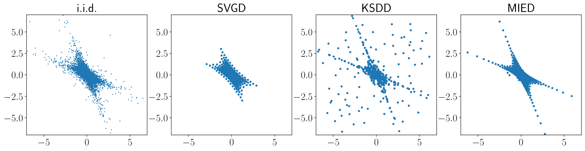
Product of two Student’s -distributions. Next, we consider a 2-dimensional distribution constructed as the product of two independent -distributions with the degree of freedom composed with a linear transform. Unlike Gaussians, Student’s -distributions have heavy tails. On the left of Figure 2, we visualize the results of each method with samples after iterations. MIED captures the heavy tail while SVGD fails. Quantitatively, on the right of Figure 2, while SVGD captures the distribution in better for , MIED yields lower metrics for a bigger .
Bayesian logistic regression. We compare MIED with SVGD and KSDD for the Bayesian logistic regression setting in Liu & Wang 2016. We further include a naïve baseline, independent particle descent (IPD), which simply runs gradient descent independently on each particle to maximize the posterior probability. In addition to using test accuracy as the metric, we include distance and energy distance between the samples from each method and samples from NUTS (Hoffman et al. 2014) after sufficient burn-in steps. We summarize the results in Table 1. All methods, including the naïve baseline IPD, are comparable in terms of test accuracy. In other words, accuracy is not a good metric for comparing the quality of posterior samples. Bayesian inference is typically preferred over maximum a posteriori estimation for its ability to capture uncertainty. When evaluating the quality of the uncertainty of the samples using distances between distributions, MIED provides the best approximation in terms of the distance and all methods (except IPD) are comparable in terms of the energy distance.
| Dataset | NUTS | IPD | SVGD | KSDD | MIED |
| banana () | 0.55 | -6.14/-3.58/0.55 | -7.81/-5.24/0.55 | -8.24/-5.76/0.55 | -7.37/-5.06/0.55 |
| breast cancer () | 0.64 | -1.51/-1.03/0.60 | -1.62/-2.06/0.60 | -1.71/-2.23/0.60 | -1.99/-2.18/0.60 |
| diabetis () | 0.78 | -2.18/-1.55/0.77 | -3.09/-3.42/0.77 | -2.91/-3.90/0.77 | -3.11/-3.13/0.77 |
| flare solar () | 0.59 | 3.30/2.65/0.48 | 6.91/4.09/0.52 | 1.77/-0.08/0.55 | 7.09/4.25/0.48 |
| german () | 0.65 | -1.80/-1.25/0.65 | -1.89/-2.63/0.64 | -1.27/-2.83/0.65 | -1.96/-2.80/0.65 |
| heart () | 0.87 | -0.40/-0.56/0.87 | -0.41/-1.50/0.87 | -0.10/-1.76/0.87 | -0.92/-1.67/0.87 |
| image () | 0.82 | 6.53/4.31/0.83 | 7.17/4.01/0.83 | 2.16/-0.50/0.82 | 1.14/-1.88/0.82 |
| ringnorm () | 0.77 | -3.82/-2.45/0.77 | -4.11/-5.98/0.77 | 1.07/-2.21/0.76 | -4.03/-5.70/0.77 |
| splice () | 0.85 | -1.47/-1.18/0.85 | -1.22/-2.65/0.85 | 2.04/-0.05/0.84 | 1.45/0.70/0.82 |
| thyroid () | 0.84 | 1.95/0.53/0.84 | 1.17/-0.00/0.84 | 2.42/1.57/0.74 | 0.84/-0.37/0.84 |
| titanic () | 0.40 | -1.59/-0.16/0.40 | -0.46/-0.31/0.40 | -0.63/-0.39/0.40 | -1.00/-0.45/0.40 |
| twonorm () | 0.97 | -1.21/-1.13/0.97 | -1.32/-2.78/0.97 | 1.55/-0.62/0.97 | -1.44/-3.21/0.97 |
| waveform () | 0.77 | -2.67/-1.87/0.78 | -2.98/-5.23/0.78 | -2.60/-4.18/0.77 | -3.09/-3.17/0.78 |
5.2 Constrained sampling
Uniform sampling in 2D. We consider uniform sampling in the square with particles. We reparameterize our particles using to eliminate the constraint and show results with various choices of mollifiers—we always choose the smallest while the optimization remains stable. We compare our method with mirror LMC (Zhang et al. 2020) and SVMD/MSVGD by Shi et al. 2021 using entropic mirror map . To demonstrate that SVGD and KSDD break down in constrained domains, we implement these two methods adapted to the constrained setting using the same reparameterization as our method. The initial particles are drawn uniformly from .
The left plot of Figure 3 shows that quantitatively our method achieves much lower energy distance and distance (compared to a i.i.d. samples uniformly drawn in .). On the right of Figure 3, we visualize the samples from each method. We see that samples from SVGD with an adaptive kernel collapse—we investigate this issue in Section D.2. Samples from SVGD with a fixed kernel size and KSDD are non-uniform (we choose kernel sizes that produce the best result). While SVMD creates locally clustered artifacts, MSVGD produces good results. For mirror LMC, the resulting samples are not evenly spaced, resulting in worse distances. When using as the reparameterization map, MIED produces decent results for all three families of mollifiers (Riesz, Gaussian, Laplace). When using the same entropic mirror map, MIED also produces good results. This highlights the flexibility of our method with constraint handling, whereas, for LMC and SVMD/MSVGD, the mirror map has to be chosen carefully to be the gradient of a strongly convex function while capturing the constraints.
In Section D.3, we further test SVMD/MSVGD with a different choice of the mirror map where they break down. In Section D.4, we conduct a similar comparison for sampling from a 20-dimensional Dirichlet distribution using the same setup as Shi et al. 2021. In scenarios where a good choice of a mirror map is available, SVMD/MSVGD can obtain better performance compared to MIED. In Section D.6, we conduct additional qualitative experiments for MIED, demonstrating its effectiveness for challenging constraints and multi-modal distributions.
Fairness Bayesian neural networks. We train fair Bayesian neural networks to predict whether the annual income of a person is at least with gender as the protected attribute using the Adult Income dataset (Kohavi et al. 1996). We follow the same setup as in Liu et al. 2021 where the dataset consists of feature vectors , labels (whether the income is ), and genders (protected attribute). The target density is taken to be the posterior of logistic regression with a two-layer Bayesian neural network with weights , and we put a standard Gaussian prior on each entry of independently. Given , the fairness constraint is . On the left of Figure 4, we plot the trade-off curve of the result obtained using our method and the methods from Liu et al. 2021 for . Details can be found in Section D.7. Our method recovers a much larger Pareto front compared to the alternatives. On the right of Figure 4, we visualize the curves of the energy and the covariance versus the number of training iterations: as expected we see a smaller results in bigger MIE (lower log-likelihood) and smaller covariance between the prediction and the protected attribute.
6 Conclusion
We present a new sampling method by minimizing MIEs discretized as particles for unconstrained and constrained sampling. This is motivated by the insight that MIEs converge to divergence with respect to the target measure as the mollifier parameter goes to 0. The proposed method achieves promising results on the sampling problems we consider.
Below we highlight three limitations. First, as discussed in Remark A.10, our theory only applies when the domain is full-dimensional or flat. Extending our theory to handle cases where the domain is an arbitrary -rectifiable set is an important next step as it allows the handling of more complicated constraints such as nonlinear equality constraints. Secondly, when , the minimizer of MIE can be different from the target measure. Finding a way to debias MIE (e.g., like how Sinkhorn distances are debiased (Feydy et al. 2019)) is an interesting direction. Lastly, the connection between the minimizers of the discretized MIE (6) and those of the continuous MIE (2) is only established in the limit as . We hope to investigate how well the empirical distribution of particles minimizing (6) approximates the target measure when is finite as in Xu et al. 2022.
Reproducibility statement.
We provide self-contained proofs in Appendix A for the theoretical results stated in the main text. The source code for all experiments can be found at https://github.com/lingxiaoli94/MIED.
Acknowledgements
Qiang Liu would like to acknowledge the support of NSF CAREER 1846421 and ONR. The MIT Geometric Data Processing group acknowledges the generous support of Army Research Office grants W911NF2010168 and W911NF2110293, of Air Force Office of Scientific Research award FA9550-19-1-031, of National Science Foundation grants IIS-1838071 and CHS-1955697, from the CSAIL Systems that Learn program, from the MIT–IBM Watson AI Laboratory, from the Toyota–CSAIL Joint Research Center, from a gift from Adobe Systems, and from a Google Research Scholar award.
References
- Ahn & Chewi (2021) Kwangjun Ahn and Sinho Chewi. Efficient constrained sampling via the mirror-langevin algorithm. Advances in Neural Information Processing Systems, 34:28405–28418, 2021.
- Ambrosio et al. (2005) Luigi Ambrosio, Nicola Gigli, and Giuseppe Savaré. Gradient flows: in metric spaces and in the space of probability measures. Springer Science & Business Media, 2005.
- Balasubramanian et al. (2022) Krishna Balasubramanian, Sinho Chewi, Murat A Erdogdu, Adil Salim, and Shunshi Zhang. Towards a theory of non-log-concave sampling: first-order stationarity guarantees for langevin monte carlo. In Conference on Learning Theory, pp. 2896–2923. PMLR, 2022.
- Blanchard et al. (2021) Pierre Blanchard, Desmond J Higham, and Nicholas J Higham. Accurately computing the log-sum-exp and softmax functions. IMA Journal of Numerical Analysis, 41(4):2311–2330, 2021.
- Blei et al. (2017) David M Blei, Alp Kucukelbir, and Jon D McAuliffe. Variational inference: A review for statisticians. Journal of the American statistical Association, 112(518):859–877, 2017.
- Borodachov et al. (2019) Sergiy V Borodachov, Douglas P Hardin, and Edward B Saff. Discrete energy on rectifiable sets. Springer, 2019.
- Brooks et al. (2011) Steve Brooks, Andrew Gelman, Galin Jones, and Xiao-Li Meng. Handbook of markov chain monte carlo. CRC press, 2011.
- Brubaker et al. (2012) Marcus Brubaker, Mathieu Salzmann, and Raquel Urtasun. A family of mcmc methods on implicitly defined manifolds. In Artificial intelligence and statistics, pp. 161–172. PMLR, 2012.
- Byrne & Girolami (2013) Simon Byrne and Mark Girolami. Geodesic monte carlo on embedded manifolds. Scandinavian Journal of Statistics, 40(4):825–845, 2013.
- Carrillo et al. (2014) José Antonio Carrillo, Young-Pil Choi, and Maxime Hauray. The derivation of swarming models: mean-field limit and wasserstein distances. In Collective dynamics from bacteria to crowds, pp. 1–46. Springer, 2014.
- Chewi et al. (2020) Sinho Chewi, Thibaut Le Gouic, Chen Lu, Tyler Maunu, and Philippe Rigollet. Svgd as a kernelized wasserstein gradient flow of the chi-squared divergence. Advances in Neural Information Processing Systems, 33:2098–2109, 2020.
- Chizat (2022) Lenaic Chizat. Sparse optimization on measures with over-parameterized gradient descent. Mathematical Programming, 194(1):487–532, 2022.
- Craig et al. (2022) Katy Craig, Karthik Elamvazhuthi, Matt Haberland, and Olga Turanova. A blob method method for inhomogeneous diffusion with applications to multi-agent control and sampling. arXiv preprint arXiv:2202.12927, 2022.
- Durmus et al. (2019) Alain Durmus, Szymon Majewski, and Błażej Miasojedow. Analysis of langevin monte carlo via convex optimization. The Journal of Machine Learning Research, 20(1):2666–2711, 2019.
- Feydy et al. (2019) Jean Feydy, Thibault Séjourné, François-Xavier Vialard, Shun-ichi Amari, Alain Trouvé, and Gabriel Peyré. Interpolating between optimal transport and mmd using sinkhorn divergences. In The 22nd International Conference on Artificial Intelligence and Statistics, pp. 2681–2690. PMLR, 2019.
- Friedrichs (1944) Kurt Otto Friedrichs. The identity of weak and strong extensions of differential operators. Transactions of the American Mathematical Society, 55(1):132–151, 1944.
- Gong & Liu (2021) Chengyue Gong and Xingchao Liu. Bi-objective trade-off with dynamic barrier gradient descent. NeurIPS 2021, 2021.
- Gorham & Mackey (2017) Jackson Gorham and Lester Mackey. Measuring sample quality with kernels. In International Conference on Machine Learning, pp. 1292–1301. PMLR, 2017.
- Hoffman et al. (2014) Matthew D Hoffman, Andrew Gelman, et al. The no-u-turn sampler: adaptively setting path lengths in hamiltonian monte carlo. J. Mach. Learn. Res., 15(1):1593–1623, 2014.
- Hörmander (2015) Lars Hörmander. The analysis of linear partial differential operators I: Distribution theory and Fourier analysis. Springer, 2015.
- Joseph et al. (2019) V Roshan Joseph, Dianpeng Wang, Li Gu, Shiji Lyu, and Rui Tuo. Deterministic sampling of expensive posteriors using minimum energy designs. Technometrics, 2019.
- Kingma & Ba (2014) Diederik P Kingma and Jimmy Ba. Adam: A method for stochastic optimization. arXiv preprint arXiv:1412.6980, 2014.
- Klenke (2013) Achim Klenke. Probability theory: a comprehensive course. Springer Science & Business Media, 2013.
- Kohavi et al. (1996) Ron Kohavi et al. Scaling up the accuracy of naive-bayes classifiers: A decision-tree hybrid. In Kdd, volume 96, pp. 202–207, 1996.
- Korba et al. (2020) Anna Korba, Adil Salim, Michael Arbel, Giulia Luise, and Arthur Gretton. A non-asymptotic analysis for stein variational gradient descent. Advances in Neural Information Processing Systems, 33:4672–4682, 2020.
- Korba et al. (2021) Anna Korba, Pierre-Cyril Aubin-Frankowski, Szymon Majewski, and Pierre Ablin. Kernel stein discrepancy descent. In International Conference on Machine Learning, pp. 5719–5730. PMLR, 2021.
- Kühn (2016) Franziska Kühn. Probability and heat kernel estimates for lévy (-type) processes. 2016.
- Liu & Zhu (2018) Chang Liu and Jun Zhu. Riemannian stein variational gradient descent for bayesian inference. In Proceedings of the AAAI Conference on Artificial Intelligence, volume 32, 2018.
- Liu (2017) Qiang Liu. Stein variational gradient descent as gradient flow. Advances in neural information processing systems, 30, 2017.
- Liu & Wang (2016) Qiang Liu and Dilin Wang. Stein variational gradient descent: A general purpose bayesian inference algorithm. Advances in neural information processing systems, 29, 2016.
- Liu et al. (2021) Xingchao Liu, Xin Tong, and Qiang Liu. Sampling with trusthworthy constraints: A variational gradient framework. Advances in Neural Information Processing Systems, 34:23557–23568, 2021.
- Pronzato & Zhigljavsky (2021) Luc Pronzato and Anatoly Zhigljavsky. Minimum-energy measures for singular kernels. Journal of Computational and Applied Mathematics, 382:113089, 2021.
- Salim et al. (2022) Adil Salim, Lukang Sun, and Peter Richtarik. A convergence theory for svgd in the population limit under talagrand’s inequality t1. In International Conference on Machine Learning, pp. 19139–19152. PMLR, 2022.
- Serfaty (2020) Sylvia Serfaty. Mean field limit for coulomb-type flows. Duke Mathematical Journal, 169(15):2887–2935, 2020.
- Shi et al. (2021) Jiaxin Shi, Chang Liu, and Lester Mackey. Sampling with mirrored stein operators. arXiv preprint arXiv:2106.12506, 2021.
- Székely & Rizzo (2013) Gábor J Székely and Maria L Rizzo. Energy statistics: A class of statistics based on distances. Journal of statistical planning and inference, 143(8):1249–1272, 2013.
- Tibshirani (2017) Ryan J Tibshirani. Dykstra’s algorithm, admm, and coordinate descent: Connections, insights, and extensions. Advances in Neural Information Processing Systems, 30, 2017.
- Trillos & Sanz-Alonso (2020) Nicolas Garcia Trillos and Daniel Sanz-Alonso. The bayesian update: variational formulations and gradient flows. Bayesian Analysis, 15(1):29–56, 2020.
- Varadhan (2001) SR Srinivasa Varadhan. Probability theory. Number 7. American Mathematical Soc., 2001.
- Wibisono (2018) Andre Wibisono. Sampling as optimization in the space of measures: The langevin dynamics as a composite optimization problem. In Conference on Learning Theory, pp. 2093–3027. PMLR, 2018.
- Xu et al. (2022) Lantian Xu, Anna Korba, and Dejan Slepcev. Accurate quantization of measures via interacting particle-based optimization. In International Conference on Machine Learning, pp. 24576–24595. PMLR, 2022.
- Xu (2021) Wenkai Xu. Generalised kernel stein discrepancy (gksd): A unifying approach for non-parametric goodness-of-fit testing. arXiv preprint arXiv:2106.12105, 2021.
- Zhang et al. (2020) Kelvin Shuangjian Zhang, Gabriel Peyré, Jalal Fadili, and Marcelo Pereyra. Wasserstein control of mirror langevin monte carlo. In Conference on Learning Theory, pp. 3814–3841. PMLR, 2020.
Appendix A Detailed Analysis
A.1 Preliminaries on mollifiers
Proposition A.1.
For , the -Riesz family of mollifiers, defined as , satisfies Definition 3.1.
In order to prove Proposition A.1, we first prove a lemma.
Lemma A.2.
Let . Then for any ,
| (8) |
where is the volume of the -dimensional sphere.
Furthermore, assuming , then for any ,
| (9) |
Proof.
If , then
where the last integral uses . ∎
Proof of Proposition A.1.
It is clear that (a) of Proposition A.1 holds for . Since is bounded we have . For any , we have, for ,
where we use (8) with and is a constant depending only on . On the other hand, using (9) with ,
where depends only on . With , we see that so (b) is satisfied.
Since is fixed and , we see that
Since , we have shown (c). ∎
In the rest of this section, we assume is a family of mollifiers satisfying Definition 3.1.
Lemma A.3.
For any , for any , and . holds.
Proof.
Assume since both cases are covered in the assumptions. Then for any , by Hölder’s inequality,
Similarly,
Letting and applying (c) gives . ∎
Proposition A.4.
Let , . Then for every , the integral
exists, so that is finite. Moreover, if is continous at , then
| (10) |
Proof.
Observe that by Hölder’s inequality, for such that (allowing infinity),
Hence is integrable and finite.
For any , note that
Since , we have
Corollary A.5.
Let , , be a continuous function. If is a sequence of functions that converge uniformly to , then for every ,
| (11) |
Proof.
Note that
Proposition A.4 shows the second term goes to as . For the first term, we have
by uniform convergence. ∎
Lemma A.6.
For , , we have
where we use to denote the translated function .
Proof.
Fix . It is a standard fact that is dense in . Hence there exists such that . Since is continuous with compact support, it is uniform continuous. Then there exists with if . Hence for such we have with . Thus
∎
Proposition A.7.
Let , . Then for every ,
In particular, . Moreover,
Proof.
For every , we have
where we use Jensen’s inequality with the observation that is a probability measure and Tonelli’s theorem to exchange the order of integration. To show the first claim, note that,
Hence .
For the second claim, by Lemma A.6, the function is continuous at with limit . Hence by Proposition A.4, we are done by taking . ∎
A.2 Convergence to -divergence
We start by giving an alternative formula for divergence with respect to the target measure.
Lemma A.8.
Define a functional by
| (12) | ||||
Then for every ,
Proof.
If is not absolutely continuous with respect to , then both sides are infinity. Otherwise, and has some density . We then compute
∎
Proof of Theorem 3.3.
Since , we know , so . We let be the density of which satisfies for . We compute using Tonelli’s theorem (since our integrand is positive):
| (13) |
where we define on and for . Moreover, by Lemma A.8,
The assumption then implies . By Proposition A.7, we have . Next notice that
This shows the first claim. Finally, the last expression goes to as since by Proposition A.7. ∎
Remark A.9.
One may ask if similar results as Theorem 3.3 for -divergences other than divergence can be obtained using similar techniques. We think the proof of Theorem 3.3 is highly specific to divergence because in (13) there are two copies of coming from the definition of as a double integral over . An -divergence between and has the form , and the only way to have showing up is to choose corresponding to divergence.
Remark A.10.
It is possible to prove versions of Theorem 3.3 when has Hausdorff dimension : in such cases -divergence still makes sense as does (2). When is “flat”, i.e., with Hausdorff dimension and contained in a -dimensional linear subspace of , e.g., when is defined by a set of linear inequalities, then Theorem 3.3 follows if we adapt the assumptions of Definition 3.1 and calculation in the proof of Theorem 3.3 to be in the subspace. For a general -dimensional , a similar calculation yields For a similar argument to go through, we will need the normalizing constant to the same for all . This is true when is a -dimensional sphere, but for a general the last integral will depend on the base point . Proving a version of Theorem 3.3 for with Hausdorff dimension is an interesting future direction.
A.3 Convexity and -convergence
We start by recalling a few definitions regarding functionals in .
Definition A.11.
We say a functional is proper if there exists such that , and is lower semicontinuous (l.s.c.) if for any weakly convergence sequence , we have .
Lemma A.12.
For any , the functional is proper and l.s.c. Moreover, if is compact, the minimum is attained by some measure in .
Proof.
Taking any , since is bounded and , we see that so is proper. Moreover, given weakly convergence , by Portmanteau theorem and the fact that is nonnegative and l.s.c., we conclude that is also l.s.c.
The set of probability distributions is tight by the compactness of . It is closed since if weakly converges to , then by Portmanteau theorem, so that . Hence by Prokhorov’s theorem (Theorem 5.1.3 (Ambrosio et al. 2005)), is (sequentially) compact. It is then an elementary result that any l.s.c. function attains its minimum on a compact set. ∎
We next prove Proposition 3.5 regarding the convexity of and the uniqueness of its minimum.
Proof of Proposition 3.5.
Let be any finite signed Borel measure. The compactness assumption and the fact that imply for any for some . Hence , so the weighted measure defined by is also finite. By the definition of i.s.p.d. kernels, we have if is not the zero measure, which is equivalent to not being zero since . Thus is i.s.p.d. on . Also note that for all , so is always finite. By Lemma 1.1 of Pronzato & Zhigljavsky 2021, we conclude that is strictly convex in , the space of finite signed measures, and in particular it is convex on . Hence combined with the existence result from Lemma A.12 we conclude attains a unique minimum in . ∎
Our goal in the rest of this section is to prove the -convergence of to defined in (12). By Lemma A.8, we have . Hence together we will have proved Theorem 3.6.
Definition A.13 (-convergence).
A sequence of functionals is said to -converge to , denoted as , if:
- (a)
For any sequence converging weakly to , ;
- (b)
For any , there exists a sequence converging weakly to with .
We will show using Fourier transforms and Bochner’s theorem.
Definition A.14 (Fourier transform).
For , its Fourier transform is the complex-valued function defined via
More generally, for a signed finite measure , its Fourier transform is the complex-valued function defined via
This integral is always well-defined and moreover is uniformly continuous; see Borodachov et al. 2019.
We will prove the following weak version (under the additional assumption that a mollifier is integrable) of Bochner’s theorem suitable for our case. In particular we will need the Fourier inversion formula which is not given in the usual statement of Bochner’s theorem. On the other hand, we cannot directly use the Fourier inversion formula since it is not obvious how to check the integrability of when is a mollifier.
Lemma A.15.
Suppose is even, bounded, continuous, and is i.s.p.d. on any compact sets. Then its Fourier transform is real, nonnegative, and the following inversion formula holds:
Proof.
The proof is adapted from that of Varadhan 2001 and is extended to the multi-dimensional case.
Since and , with a change of variable , we obtain , so is real.
Next we show that is nonnegative. For , we compute, for a fixed ,
where we have used change of variable , . Since , by dominated convergence theorem, we have as
For , we have
For a fixed , if we define a finite measure as , then being i.s.p.d. implies
and similarly for . Since is real, we conclude that is nonnegative.
Finally we prove Lemma A.15. For , define . Since is bounded (because ), we see that . We compute, for , using Fubini’s theorem,
where we use the Fourier transform formula (Borodachov et al. 2019, (4.4.1)) of the Gaussian distribution. Notice that is the density of a multivariate Gaussian centered at with covariance . Hence . Since is bounded by assumption, with we find . Taking , by monotone convergence theorem, we have , so together with the fact that we have . Finally, since , by dominated convergence theorem and Proposition A.4 (note is centered at ), we have
∎
Proposition A.16.
Given satisfying the assumptions of Lemma A.15, for any , it holds that
Proof.
By Lemma A.15,
where we use Fubini’s theorem (all measures are finite and is bounded) to exchange the order of integration. ∎
Proof of Theorem 3.6.
First note that Definition A.13(b) is immediate from Theorem 3.3 with : if , then trivially ; otherwise we apply Theorem 3.3. So we focus on proving criterion Definition A.13(a).
Fix a sequence that converges weakly to , and our goal is to show . Without loss of generality, we may assume for all (these terms have no effect in ), which implies . By Portmanteau’s theorem and the assumption that is closed, we have . So all of and will have support in .
For , define a nonnegative measure by
where is a continuous monotonically decreasing cutoff function satisfying if and if , and that for . Then since is continuous, it is bounded below on any compact set in , and hence is finite. Also define, for , a nonnegative measure by
which is again finite following the same reasoning.
Then for any , denoting ,
| (15) |
where we apply Proposition A.16 for the last equality. On the other hand, note that
Since weakly and the last integrand is a continuous bounded function, we have
On the other hand, . Since by Definition 3.1, converges to in probability (and in particular weakly), we have .
Applying Fatou’s lemma to (15), we obtain, for any ,
If for any , then we are done since . Otherwise, by Kühn 2016, for every , has density in . This imples has density everywhere. Suppose . By Plancherel’s theorem and the monotone convergence theorem, we have
This completes the proof of .
Now suppose is compact, and let . To establish weakly (resp. ), it suffices to show that every subsequence of (resp. ) has a further convergence subsequence converging to (resp. ). With a slight abuse of notation, we assume the sequence of is chosen so that (resp. ) is already some subsequence of the original sequence. As argued in the proof of Lemma A.12, is compact with respect to weak convergence. Hence has a weakly convergence subsequence for some . The -convergence implies
where we have used, for each inequality, , Definition A.13(a), the first paragraph of this proof, and again the fact that . Since by Theorem 3.3, we have
where the last inequality follows because is the minimizer of . Then . Moreover, . This can only happen if and agree on all Borel sets, so . ∎
A.4 Differential calculus of in
Lemma A.17.
Let , , and be a compact set. Suppose is jointly continuous and the derivative exists and is jointly continuous. Then is differentiable for , and
where the integration is with respect to the Lebesgue measure on .
Proof.
Fix and let be small enough such that . Note that is well-defined by the dominated convergence theorem since and . Define which is finite since is continuous, so that for all and is integrable since . Hence by the differentiation lemma (Klenke 2013, Theorem 6.28) we are done. ∎
The following lemma is similar to Korba et al. 2021 but with different assumptions: we do not put any integrability assumptions on , but we do restrict measures to have compact support. For a differentiable , we use to denote the gradient with respect to . We also use to denote the Hessian of with respect to . We similarly denote and .
Lemma A.18.
Assume has density . Let . Denote . Then for all and all ,
| (16) |
In particularly,
| (17) |
Moreover,
| (18) |
Proof.
We compute
Since has compact support and is jointly continuous and its derivative with respect to is also jointly continuous, by Lemma A.17, we can push inside the double integral and we obtain (16). Another application of Lemma A.17 shows that if we take derivative with respect to again on (16) and evaluate at we obtain (18). ∎
Lemma A.19.
Let , . Assume has compact support for some . Then for all , is differentiable and
Proof.
Since is compact and is bounded on any compact set, we know is well-defined at every . Note that
Since is compact and is , by Lemma A.17 we justify the existence of the derivative and the exchange of differentiation and integration (?). ∎
A.4.1 Subdifferentials of
Recall the following notion of a “Wasserstein gradient” in from Ambrosio et al. 2005.
Definition A.20.
A vector field is a strong Fréchet subdifferential of a functional if for all , the following holds:
| (19) |
Note that we cannot apply Ambrosio et al. 2005 directly to prove (4) because interaction energies cannot be written in the form of (10.4.1) in their setup.
Proof of Proposition 3.7.
Let . By Lemma A.18, we have
where the last step follows from applying Lemma A.17 since has compact support. Now suppose is a strong Fréchet subdifferential satisfying (19). For the sequence , we have by definition
Hence
The previous calculation shows exists, and hence it is equal to . This proves for any ,
Hence we have shown (4).
Finally, we show for -a.e. under the additional assumption that has compact support. By Ambrosio et al. 2005 with , we find the strong subdifferential of is given by
| (20) |
To show (5), we compute, for -a.e. ,
where for the last equality we have applied Lemma A.19. Now taking , by Proposition A.4 using the fact that is compact (so that and are bounded on ), we obtain (5). ∎
A.4.2 Displacement convexity of at as
The statement of Proposition 3.8 is similar in form as Korba et al. 2021 but in our case we do not have the second term in Equation 18 vanishing and we need to take the limit . We also do not resort to RKHS theory in the proof.
Proof of Proposition 3.8.
By (18), we have
where
We tackle first. Observe that successive application of integration by parts using the fact that has compact support gives
If we view as the density of a signed measure (it is integrable since it has compact support), and since is i.s.p.d. on the support of by Proposition 3.5(a), we see that each double integral in the last expression is non-negative. Hence .
Next we show . Since has compact support, by Fubini’s theorem,
To expand the integral inside the Hessian operator, we have
First by the chain rule and Lemma A.19, we have
Differentiating again while applying Lemma A.19, we obtain after rearranging terms,
| (21) |
By Proposition A.4 and the fact that , we have
Finally, we have
where interchanging the limit and the integral is jusfitied by the dominated convergence theorem and the fact that and have compact support (we need compact support assumption of to make sure convolutions appearing in (21) are uniformly bounded when is sufficiently small).
∎
A.4.3 A descent lemma for with time discretization
We now consider a time discretization of the gradient flow of given by, for an initial measure and , with a step size ,
| (22) |
Similar to Korba et al. 2021, we can show the following descent lemma for iterations (22) with the following additional assumptions:
Assumption A.21.
Suppose the target density satisfies , , for some for all , where we use to indicate the matrix spectral norm (i.e. ). Suppose the mollifier satisfies, in addition to Definition 3.1, , , and for some , , .
Lemma A.22.
Under A.21, there exists a constant such that the function is -Lipschitz in terms of in either input.
Proof.
Denote . Then our assumptions imply , , and . We compute, for ,
Then
and
Then we have
Hence we conclude that is -Lipschitz with
∎
Remark A.23.
Compared with Korba et al. 2021, to ensure is Lipscthiz, we only require uniform boundedness of and up to second order derivatives instead of up to order 3.
Proposition A.24.
Under A.21, suppose has compact support. Then for any , with defined as in Lemma A.22 and defined as in (22),
| (23) |
Proof.
We first show has compact support for all . For with compact support, the proof of Proposition 3.7 implies (note Proposition 3.7 assumes has density but it is not necessary to obtain the following formula using the same proof)
Since is by the assumptions and has compact support, by Lemma A.17, we see that is differentiable with
By induction, suppose has compact support. Then
Since is continuous, the set on the right-hand side is bounded. Hence has compact support.
Now fix and we show (23). Define a path defined by . Let . By Lemma A.18, the continuity of implies that is differentiable. Moreover, another application of Lemma A.17 implies that is twice differentiable, and in particular continuously differentiable. Hence is absolutely continuous on the compact interval . By the fundamental theorem of calculus, we have
Observe that by Lemma A.18,
where we apply Fubini’s theorem to exchange the order of integration together with the fact that has compact support and the integrand is continuous. Let . Note that, again by Lemma A.18,
Note that, by Lemma A.22, we have
Thus
where we have used the Cauchy-Schwartz inequality in the last step.
Combining everything, we have shown
since .
∎
Appendix B Weighted hypersingular Riesz energy
We recall results most relevant to us from Borodachov et al. 2019. Suppose is compact, of Hausdorff dimension , and -rectifiable, i.e., the image of a bounded set in under a Lipschitz mapping. Given a non-vanishing continuous probability density on , define a measure for any Borel set . The target measure is defined to be . The weighted -Riesz energy is defined as the interaction energy
| (24) |
The following result states that minimizers of the weighted -Riesz energy approximate the target measure when the is sufficiently large.
Theorem B.1 (Theorem 11.1.2, Borodachov et al. 2019).
Suppose . For with , we have weak convergence as .
A similar result with a slightly different assumption holds for (Theorem 11.1.3 of Borodachov et al. 2019).
Comparison of (24) with discretized MIE (6).
Our theory is only valid for the full-dimensional case, i.e., (see a few exceptions discussed in Remark A.10). When this is the case and if the mollifier is taken to be from the -Riesz family, (6) becomes, for ,
Compared with (24), in our case there is an in the denominator, so that the continuous version of the energy does not blow up all the time (this is in contrast with the continuous version of (24)—see Borodachov et al. 2019). Moreover, the exponential scaling on is different: in our case we use whereas in (24) it is . The diagonal is included in our energy, but this is inconsequential as another valid discretization is to discard the diagonal term (Borodachov et al. 2019, Theorem 4.2.2). On the other hand, our theory allows a bigger class of mollifiers that are not necessarily of Riesz families. We also allow to be non-compact. An interesting future research direction is to extend our theory to cases where , e.g., when is an embedded -dimensional submanifold in .
Appendix C Algorithmic details
In this section we provide algorithmic details of MIED and compare with the updates of SVGD (Liu & Wang 2016). The negative gradient of (7) with respect to is
where
| (25) |
and to get the last equality we used the fact that thanks to the assumption . Then gradient descent on (7) gives our algorithm (Algorithm 1). The special treatment of the diagonal terms described in Section 4 amounts to modifying only the diagonal .
C.1 Comparison with SVGD
The update formula in Algorithm 1 is similar to the one in SVGD: if we use in place of the kernel in the SVGD update and rewrite:
| (SVGD) |
For both algorithms, the update formula for each particle consists of attraction and repulsion terms and the total time complexity of each update iteration is . We note the following differences. First, in our formulation we have scaling factors which help stabilizing the optimization (as a by-product of working in the logarithmic domain) and put more weight on nearby particles as well as particles in low-density regions, whereas in (SVGD) the scaling factors are which are not adapted to prioritize low-density regions. Second, in MIED, the attraction force for particle only comes from , whereas in (SVGD) the attraction force comes from for all ’s. Third, for each , in our formulation the repulsive force has an additional factor of in front of .
Empirically, the additional scaling factors in MIED help produce samples with good separations compared to SVGD, since closer pairs of points will have large weights. Additionally, since MIED optimizes a finite-dimensional objective (7), we can employ accelerated gradient-based optimizers like Adam (Kingma & Ba 2014), which we used in our experiments. In contrast, SVGD does not optimize any finite-dimensional objective. While practical SVGD implementations also use optimizers like Adam, it is unclear how the resulting particle dynamics is related to the gradient flow of KL divergence.
C.2 Handling constraints with dynamic barrier method
The dynamic barrier method is introduced in Gong & Liu 2021 which solves subject to where is scalar-valued. Intuitively, their method computes update directions by either decreasing when , following if the constraints are satisfied, or balancing both gradient directions.
In order to handle multiple constraints such as in Figure 11, we consider a generalized version of their dynamic barrier method. In this generalized setting, is vector-valued and constraints are where the sign is interpreted coordinate wise.. Suppose we are at iteration with current solution . Then the next update direction is taken to be the of
| (26) |
where are fixed hyperparameters; in our implementation we simply choose . Then with learning rate . In our implementation we use Adam (Kingma & Ba 2014) that modulates the update directions. Observe that the optimization problem (26) is the same as projecting a point onto the polyhedron formed by the intersection of the halfspaces . To solve (26), we use Dykstra’s algorithm (Tibshirani 2017) which can be interpreted as running coordinate descent on the dual of (26). We use a fixed number of iterations for the Dykstra’s algorithm which we found to be sufficient for our experiments; in the case of a single constraint, we only need to use one iteration.
Appendix D Experiment details and additional results
D.1 Gaussians in varying dimensions
We generate the -dimensional Gaussians used to produce Figure 1 as follows. We generate a matrix with i.i.d. entries uniformly in . Then we set . This way . We then use as the covariance matrix for the Gaussian (centered at 0). We use Adam with learning rate for all methods for a total of 2000 iterations. This is enough for SVGD and MIED to converge, while for KSDD the convergence can be much slower.
We visualize the samples from each method for in Figure 5. We notice that MIED is capable of generating well-separated samples, while for SVGD there is a gap between the inner cluster of samples and a sparse outer ring. For KSDD we see the artifact where too many samples concentrate on the diagonal.

D.2 Collapsed samples when the kernel width is too big
In Figure 3, we see that samples from SVGD collapse with an adaptive kernel where the variance is taken to be half of the median of the squared distance among all pairs of points (Liu & Wang 2016); at termination the median of the squared distance is greater than in that experiment. Here we investigate this issue further. In Figure 6, for the same uniform sampling setup, we visualize the results of SVGD with a fixed kernel width and MIED with Gaussian mollifiers with the same kernel width: when the kernel width (i.e. in ) is too big, both SVGD and MIED result in collapsed samples. This is because since the target density is a constant, the only force in the updates is the repulsive force. When the kernel width is too large, the repulsive force coming from points in the same collapsed cluster is dominated by the repulsive force coming from points from other clusters—this is evident in the update directions shown in the leftmost column of Figure 6 (SVGD with kernel width ).
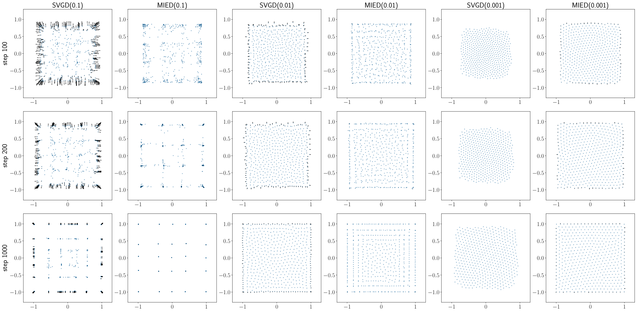
When using the dynamic barrier method Gong & Liu 2021 to enforce the square constraints instead of reparameterization with , we obtain similar results as in Figure 6.
This pathological phenomenon is not only limited to constrained sampling: when sampling the 2D Gaussian from Figure 5, using too big a kernel width can also result in collapsing (Figure 7).

We emphasize that our theory of MIED suggests that in practice we need to choose the kernel width very small in order to sample from the correct target measure according to Theorem 3.3 and Theorem 3.6. In comparison, the theory of SVGD has no such implication.
D.3 Uniform sampling with an alternative mirror map
In this section, we show that for sampling from a uniform distribution in the square , the results of SVMD/MSVGD (Shi et al. 2021) depend heavily on the choice of the mirror map. Instead of the entropic mirror map used to produce results in Figure 3, here we use the mirror map as in Ahn & Chewi 2021. The results are shown in Figure 8. SVMD/MSVGD fail to draw samples near the boundary; we suspect this is because the gradient of the conjugate (coordinate-wise arithmetic) requires coordinates of to go to to land near the boundary. We verify this phenomenon by using as the reparametrization map in MIED (rightmost figure in Figure 8): indeed with such reparameterization MIED also struggles near the boundary.
D.4 20-dimensional Dirichlet distribution
We sample from the 20-dimensional Dirichlet distribution in the same setup as in Shi et al. 2021 with 50 particles. Results and visualization are shown in Figure 9. We see that unlike sampling from a box (Figure 3), both MSVGD and SVMD by Shi et al. 2021 perform well in this experiment. This is due to the fact that the entropic mirror map used here is a well-tested choice for simplex constraint, yet obtaining a good mirror map for a generic constraint, even if it is linear, can be challenging. Our method does not have such a limitation, as it can easily incorporate existing constrained optimization tools.
D.5 Effect of for Riesz mollifiers
When we use the -Riesz families of mollifiers in MIED, we have the freedom of choosing the hyperparameter so long as . In this section, we study the effect of on the resulting samples. We consider the problem of sampling from a mixture of four 2D Gaussians centered at , each with diagonal variance and constrained to the box. We vary in and the number of particles in . All runs use a total of iterations with learning rate . In the top of Figure 10, we plot the distance and energy distance as functions of for each . Interestingly, we see the best performing is in and depends on . This suggests that our choice of in Section 5 may not be optimal and there is room for hyperparameter tuning to further improve the performance of MIED with Riesz kernel. At the bottom of Figure 10 we visualize the samples of MIED with and of SVGD with kernel width (adaptive kernels would result in collapsed samples and other widths we tested on would result in worse samples). While SVGD samples form visible artifacts, the samples of MIED are evenly distributed and the four modes of the mixtures emerge as increases.
D.6 More constrained sampling experiments
In this section we test MIED on more low dimensional constrained sampling problems and qualitatively assess the results. Note that mirror LMC (Zhang et al. 2020; Ahn & Chewi 2021) or mirror SVGD (Shi et al. 2021) cannot be applied due to non-convexity of the constraints. In Figure 11, we consider uniform sampling of a challenging 2D region with initial samples drawn from the top-right corner: as the number of iterations increases, MIED gradually propagate samples to fill up the entire region. In Figure 12, we consider sampling from a von Mises-Fisher distribution on a unit sphere. Although our theory focuses on sampling from a full-dimensional distribution, as discussed in Remark A.10, we can extend Theorem 3.3 to the case of a sphere due to its symmetry. We see the samples visualized in Figure 12 capture the two modes that emerge by restricting the Gaussian to a unit sphere.


D.7 Details on fairness Bayesian neural network experiment
We use training/test split as in Liu et al. 2021. We use the source code provided by Liu et al. 2021 with default hyperparameters.The source code provided by the authors of Liu et al. 2021 does not implement the calculation of faithfully as written in the formula, so we corrected it. All methods use 2000 iterations for training. For our method we use learning rate . One of their four methods (Control+SVGD) got stuck at initialization (with accuracy around ), so we omit its result from the plot in Figure 4.