On the failure of variational score matching
for VAE models
Abstract
Score matching (SM) is a convenient method for training flexible probabilistic models, which is often preferred over the traditional maximum-likelihood (ML) approach. However, these models are less interpretable than normalized models; as such, training robustness is in general difficult to assess. We present a critical study of existing variational SM objectives, showing catastrophic failure on a wide range of datasets and network architectures. Our theoretical insights on the objectives emerge directly from their equivalent autoencoding losses when optimizing variational autoencoder (VAE) models. First, we show that in the Fisher autoencoder, SM produces far worse models than maximum-likelihood, and approximate inference by Fisher divergence can lead to low-density local optima. However, with important modifications, this objective reduces to a regularized autoencoding loss that resembles the evidence lower bound (ELBO). This analysis predicts that the modified SM algorithm should behave very similarly to ELBO on Gaussian VAEs. We then review two other FD-based objectives from the literature and show that they reduce to uninterpretable autoencoding losses, likely leading to poor performance. The experiments verify our theoretical predictions and suggest that only ELBO and the baseline objective robustly produce expected results, while previously proposed SM methods do not.
1 Introduction
Finding robust algorithms for training expressive latent variable models remains at the heart of unsupervised learning research. Latent variable models describe the data distribution by mapping a prior distribution of latent variables through a likelihood. A well-established approach for training such models is maximum likelihood (ML) that minimizes the Kullback-Leibler divergence (KLD) between the data and model distributions. Exact ML is usually intractable in practice; instead, one optimizes a lower bound of the log-likelihood (or upper bound on the KLD) defined through a variational distribution, known as the evidence lower bound (ELBO) [14, 23]. These approaches have produced robust results across task, datasets and model architectures [15]. Score matching offers another approach to training statistical models [12]; it minimizes the Fisher divergence (FD), a convenient objective for potentially unnormalized models. When latent variables are present, a situation we focus on here, the FD can be approximated [27, 28, 2, 7].
Practitioners, who want to model their datasets under budget, see these two alternatives and naturally ask: which one is more robust so that the results are generally good without expensive hyperparameter search? KLD and FD are connected through differential relationships [26, 9, 18], but these results do not predict the robustness of using these divergences for training. Some previous work examined the difference between ML and SM in fully observed models [29, 1, 25] and latent variable models [2]; however, comparisons that control for the model class are missing. In addition, existing SM objectives that give empirical success appear similar to each other [7, 2] but their differences remain unclear. Addressing these issues gives better understand of these methods, and avoid unexpected failures and expensive hyperparameter search. Further, a well-controlled comparison can reveal whether the improvements seen previously should be attributed to training objectives or other details.
Here, we conduct such a study of variational SM objectives using variational autoencoding models (VAEs) to unveil their differences and connection. Importantly, the joint distribution of a VAE model is normalized and thus can be trained conveniently via ML and SM; as such, VAE models provide an intuitive setup for theoretical analysis and well-controlled experiments: a robust ML or SM algorithm must be capable of training a VAE on a dataset. In particular, we focus on Gaussian VAEs on which important theoretical insights have been derived and practical successes seen [5, 20, 4, 24] .
In Section 2, we review the traditional variational ML approach and its objective (ELBO). Our main contributions consist of the analyses and illustrations in Sections 3 and 4, and the experiments in Section 5. Specifically, Section 3 studies a recently proposed variational SM objective known as the Fisher autoencoder [7]. We show that this objective can perform poorly in a counterintuitive way. We then, for the purpose of comparison, introduce a benchmark SM objective that is very similar to ELBO in their equivalent autoencoding losses and is thus expected to work as well as the latter. Unfortunately, two other existing SM objectives [27, 2] do not admit any reasonable autoencoding loss Section 4. Experiments (Section 5) demonstrate that the benchmark variational SM objective gives comparable performance to ELBO on several metrics, while the other variational objectives often failed. A concluding summary and limitations of this work are discussed in Section 6.
2 Background: variational autoencoders and maximum likelihood
We analyze training objectives on VAEs in which the generative model is expressed as where is latent, is observed, and is the vector of parameters. The prior is fixed for the purpose of this study. The parameters of this model is trained using i.i.d. samples of a dataset so that the marginal is close to the underlying unknown data density . To find , maximum-likelihood (ML) optimizes the marginal KLD which is intractable for most models used in practice. A more practical approach to ML is to optimize ELBO:
| (1) |
where is a variational distribution in some prespecified distributional family . It is usually parametrized by which is independent of . It can be shown that maximizing the expected ELBO amounts to minimizing the joint KLD
| (2) |
The joint KLD is attractive for learning because it upper bounds the marginal KLD, and the variational posterior can be optimized independently of . In this work, we focus on the Gaussian VAE where the relevant densities are given by
| (3) |
Here, the functions , and specify the distribution parameters, and is a scalar variance of the likelihood. In later sections, we sometimes relax the assumption that is Gaussian. The Gaussian VAE is not only widely used in practice for modelling complex continuous data distributions but also intuitive for deriving interesting properties. For example, it can be shown [6, 4] that in the limit of small posterior variance, the ELBO on the Gaussian VAE reduces to the following autoencoding objective at its optimum
| (4) | |||
where is an increasing concave function approaching as . Importantly, [4] further showed that the unbounded gradient around zero in is necessary for learning a form of optimal sparse representation of the data. Such a property is valuable to many downstream applications that rely on efficient lower-dimensional representations. We will see how the autoencoding loss (4) is related to objectives of variational score matching in Gaussian VAEs.
3 Variational score matching
As an alternative to ML, SM minimizes the marginal FD between the data and model distributions
| (5) |
where is the Jacobian w.r.t. . Practical algorithms for fully observed models were initially proposed by [12]. Here, we consider SM algorithms for VAE models. For brevity, we define the following shorthands and .
3.1 Revisiting Fisher autoencoder
As discussed in Section 2, the joint KLD (JKLD) provides a convenient objective for approximate ML. [7] applied this intuition to SM and proposed the Fisher autoencoder (FAE) which optimizes the joint FD (JFD)
| (6) | |||
| (7) |
A derivation is given in Section A.1. The two terms in (6) arise from the partial derivatives w.r.t. and , respectively. For a fixed , if for all and , then . [7] further showed that is equal (up to a -dependent constant that can be ignored for optimization) to , where
| (8) |
is a practical objective for SM. However, unlike the KLD case (2), the JFD is not an upper bound on the marginal FD. This means that a good fit over JFD may not imply a good fit over the target marginal FD. A perfect match in the joint distributions implies a perfect match on their marginals. But when the joint distributions do not match exactly, there is generally no guarantee that the marginals will be close, unless there is a bounding relationship as in the KLD case.
For example, consider a simple VAE defined by a prior , likelihood , and a parametric variational posterior , where is the exact posterior variance for the generative model, is fixed, and the factor is used to impose posterior mismatch. Suppose we perform parameter recovery: Let the data distribution be for a ground truth , and we wish to recover by . When , the posterior is exact, and thus any setting of can be recovered. We focus on the case where and show that estimated by JFD minimization can be far away from (Figure 1, left) . On the contrary, minimizing the JKLD produced robust estimates. To further illustrate this problem, we plot and found by minimizing JKLD and JFD in Figure 1 when the true . These joints are close in JFD but not at all in JKLD or visual judgment. Therefore, minimizing JFD jointly over and [7] may be undesirable when is approximate.
3.2 Improved variational SM for semi-Gaussian VAEs
We took a closer look at the loss proposed by [7] and discovered that a simple modification can lead to an autoencoding loss similar to (4) for a wider class of VAEs. For a semi-Gaussian VAE in which only the likelihood is Gaussian but and are unspecified, we have the following proposition, derived in Section A.2.
Proposition 3.1.
Remark 3.2.
Proposition 3.1 suggests that should in fact be used as an objective for optimizing (learning) only, effectively removing the expectation under in (8). On the other hand, the objective for optimizing (inference) is unspecified. The rightmost equality in (7) indicates that if is close to zero, then roughly equals the marginal FD. Therefore, a gradient step on should not proceed until closely matches . This overall procedure does not optimize the joint FD, as in FAE [7], or upper-bounds any marginal divergence; this is unlike variational ML which optimizes the joint KLD over and and bounds the marginal KLD from above. In practice, the variational can be updated by FD or KLD, as discussed in the next subsection.
We stress the algorithm described above does not optimize the joint FD as in FAE [7], nor does it perform coordinate descent between and on the original JFD. In this procedure, is used to optimize for only, which effectively removes the second summand in the FAE objective (8); this term is also not involved in optimizing . Further, is not optimized through the posterior FD in (6). Our modification thus deviates from FAE in nontrivial ways.
3.3 Fisher divergence for inference
Training an encoder by minimizing the KLD is a popular approach for many VAE models and even jointly unnormalized models [2]. However, for real , the FAE objective (6) suggests FD as an objective for inference. While both divergences can be estimated and optimized easily for the Gaussian VAE model, it is unclear which objective should be preferred for inference. Here, we discuss properties of the solution and optimization when is optimized for FD.
3.3.1 Optimal posterior in Gaussian VAEs
For a Gaussian VAE, in situations where the data have low noise (e.g. natural images), the optimal posterior usually has small variance. In this case, as explained in Section A.4, the posterior FD approximately reduces to
| (10) |
where the optimal posterior precision of is As such, when the Gaussian VAE model is well trained and the posterior variance is small, FD as the inference objective regularizes the posterior mean in a way similar to the KLD (4). Further, the optimal in FD coincides with that in KLD as derived by [5, Equation 83]. Thus, using FD for inference can produce the same desirable effects arising from this discussed by the authors. However, Equation 10 also reveals that the optimal Gaussian still incurs nonzero FD. The joint and marginal FDs in (6) are then separated by the nonzero posterior FD Equation 10. Therefore, we expected that FD is not an ideal inference objective for learning a Gaussian VAE by JFD or .
3.3.2 Local optima in FD optimization


Having characterized the solution of FD inference on a Gaussian VAE, we now turn to optimization. [7] proposed to optimize a parametric using the unbiased reparametrization gradient. However, we were unable to produce any reasonable results with this approach, which prompted us to investigate optimization on simpler problems. Consider a generative model with a standard Gaussian prior and a likelihood in
| (11) |
The posteriors induced by these likelihoods as shown in Figure 2 (contours). To approximate these posteriors, we chose a variational family as factorized Gaussians and optimized its mean and variance on by either SGD or Adam [13], using reparametrization gradients. We visualize in Figure 2 (“FD, repar”) the trajectories of its mean when initialized at different points in the latent space. Surprisingly, for likelihood , there is a low-density local optimum at the origin that attracts variational posteriors with means initialized from the orange dots. Using Adam exacerbated this problem by enlarging the basin of attraction. A similar issue also arises in the optimization of the Stein discrepancy [16]. In contrast, minimizing the KLD did not produce such a solution (“KLD, repar”). For the likelihood , Adam also produced a local optima far away from the bulk of the posterior mass. SGD found a unique optimum regardless of initialization, but the solution was visibly different from that of KLD.
We hypothesize that the inappropriate convergence to low-density local optima is due to the gradient contribution of reparametrization: the FD can be lowered when is driven to concentrate around a small region where its shape (but not its density) roughly matches the posterior’s (i.e. is small). We test this hypothesis by optimizing without reparametrization. In Section A.5.1, we show that the FD gradient without reparametrization is more similar to the KLD gradient than reparametrized gradient for a simple problem. Indeed, for the toy problems in Figure 2, following this gradient (“FD, no repar”) resulted in more similar dynamics and final solutions to KLD inference. More importantly, the posteriors no longer converge to the bad local optima. In our experiments on image data, we could only obtain a reasonable fit by using unparametrized gradients when FD was chosen as the objective. Although some advantage arises now that inference may not require reparametrized samples (Section A.5.2), this biased gradient can be problematic, such as when is a Laplace (Section A.5.3).
Combining the results of FD-based learning and inference in Sections 3.2 and 3.3, we summarize the benchmark variational SM procedure in Algorithm 1. Since this algorithm is closely related to the ELBO (4), we expect their performances to be largely similar without hyperparameter tuning. Further practical limitations of Algorithm 1 are discussed in Section 6, and for these reasons, this algorithm is used only to benchmark with other SM objectives in VAE models. It is also distinct from FAE [7] which failed badly in all our experiments.
4 Marginal SM objectives do not recover autoencoding losses
There are two closely related variational SM objectives [27, 2]. They optimize approximations to the marginal FD (5) rather than the joint FD, with implications that we discuss in detail here. First, [27] derived an objective that is equivalent to (5) up to a -dependent constant:
| (12) |
For a VAE model, one can replace with in (12) to obtain a per-datum loss
| (13) |
In the special case of Gaussian VAEs, we applied the same technique used for Proposition 3.1 to , giving the following autoencoding loss.
Proposition 4.1.
The second term of involves the expected -2 norm of the reconstruction mean, while the second term of in (4) and (9) is the reconstruction variance. Thus, the objective proposed by [27] applied to semi-Gaussian VAEs overly constrains the reconstruction.
Second, [2] inserted the identity into the marginal FD (5), giving
| (14) |
The authors then replaced with a variational posterior . We derive its equivalent autoencoding loss below for semi-Gaussian VAEs.
Proposition 4.2.
Approximating with , the marginal FD (14) is equal to , up to a -dependent constant, where
| (15) |
In contrast to and , the autoencoding loss for is not immediately interpretable and is deferred to Section A.2 only for completeness.
Another common issue of these two objectives above is that replacing the exact posterior with a variational removes its dependence on . [2] proposed to update by -dependent gradients. Nevertheless, this inner optimization is slow in practice and was discarded in the authors’ main experiments. The contribution of this bi-level optimization is thus unclear, which we test empirically in Section 5. In contrast, the FAE based on the joint FD and Algorithm 1 based on our benchmark objective use a free variational posterior independent of .
5 Experiments
To compare the effects of training objectives on Gaussian VAE models, we tested All combinations of the two inference objectives (KLD and FD) and the three SM objectives (’s), yielding six overall SM objectives. The ELBO objectives is used as a baseline. Note that [2] used an objective that is equal to - in expectation. Optimizing FD with reparametrized gradient, or optimizing the joint FD as in Fisher autoencoder [7] did not give any reasonable results and are excluded for detailed comparison. The goal of these experiments is to confirm the analyses in previous sections. In particular, we expect that is the only learning objective that can produce results similar to ELBO, and the other learning objectives are worse. Thus, we also do not expect the benchmark algorithm or any previous methods applied to VAEs to achieve state-of-the-art performance on any standard metrics. Details are in Appendix B and code is available at github.com/kevin-w-li/LatentScoreMatching.
5.1 Synthetic datasets
We first trained Gaussian VAEs composed of fully connected layers (two hidden layers of 30 units) on simple 2D datasets. The latent space is . For each combined objective, we ran gradient updates to the encoder before updating the decoder. For objectives involving and where bi-level optimization is required, we also updated the encoder times with gradients that retain its dependence on . The gradient for each update is computed using a minibatch of 1 000 samples. Each experimental setting is repeated 10 times. After training, the trained models are evaluated by the negative log-likelihood (NLL) and score matching loss (FD minus a constant) on unseen data, approximated by importance sampling using samples.
The results are shown in Figure 3. The ELBO objective (-ELBO) and - produced almost equally good results, both the NLL and FD decrease as the number of encoder updates increases, as expected. This confirms our analysis that these two objectives optimize very similar autoencoding losses. On the other had, - is slightly worse, suggesting that the Fisher divergence is indeed not an ideal objective for learning . The objectives involving and could not fit the model well. The NLL and FD for objectives were above the limits of the figure axis ranges. On these two synthetic datasets, we did not observe strong positive effects of bi-level optimization. But we did observe this effect for much higher , and network size; see Section B.1 where results on other synthetic datasets are also reported.

5.2 Benchmark datasets
Procedure
We tested the variational SM on the Gaussian VAE model MNIST [17, CC BY-SA 3.0] and FashionMNIST [30, MIT] and CelebA [19, CC-BY-4.0] datasets. All images are resized to . To avoid potentially unbounded gradients as , we added a small Gaussian noise to the data. This also prevented gross overfitting. Two neural architectures were tested: ConvNets as defined in DCGAN [21] and ResNets [10]. To ensure a good posterior approximation, we drew samples from to estimate expectations and updated times for every update. We did not perform bi-level optimization for large benchmark datasets [2]. Adam with step size was used as the optimization routine, and training lasted 1 000 epochs for each objective on each dataset. These experiments were run on NVIDIA® GTX 1080 GPUs.
To make a thorough comparison between the training objectives, we computed the following metrics on the test dataset after every 10 epochs: a) the negative ELBO as an overall metric; b) reconstruction mean squared error (MSE); c) the latent maximum mean discrepancy [8] between the aggregate posterior and , a global measure of the posterior approximation; and d) the average FD between the approximate and exact posteriors, a local measure of the posterior approximation. We also computed the FID [11] and KID [3], measuring sample quality, after training. Note that the latent MMD and the average posterior FD may increase through training as the true becomes more complicated.
ConvNets
We focus on the results of ConvNets shown in Figure 4. The benchmark objective - gave learning trajectories almost identical to the -ELBO on all metrics for all datasets. - produced the best negative ELBO compared to the other - objectives but is still worse than -ELBO or -. These are again consistent with our analyses. Comparing between the SM objectives, we found that and underperform -ELBO and on negative ELBO and latent MMD. gave the highest reconstruction error, which may be the result of Proposition 4.1 that predicts over regularization of the reconstruction mean. produced the lowest reconstruction MSE on the MNIST dataset only, but the latent MMD and posterior FD is large on other datasets.
Regarding inference, - gave the lowest latent MMD on Fashion and CelebA, and - gave the lowest posterior FD on CelebA. However, overall, methods with FD-based inference fared worse on latent MMD and posterior FD than those with -based inference. Thus, KLD is indeed the preferred objective for variational learning even when the learning objective is FD, as done in [2]. The sample qualities are shown in Table 1. +ELBO and the benchmark gave some of the best FIDs. Again, - produced indistinguishable results compared to +ELBO, but other objectives yielded worse FIDs.
ResNets
So far, the empirical results are consistent across dataset, networks and different runs of the same settings. What if the VAE uses the more flexible ResNets? We focus on the sample quality metrics in (Table 1) and defer more detailed results to Section B.2. - produced better samples than -ELBO on all datasets. The combination - had better sample quality than - and -ELBO (Table 1) on MNIST. Surprisingly, the best sample quality model turned out to be -, although all - combinations produced the worst negative ELBO, reconstruction error and posterior FD than - combinations (Section B.2). These results suggest strong effects of neural architecture on performance when is used. In principle, using this objectives for training the decoder would require a bi-level optimization over , but in practice this does not seem necessary when ResNets are used, as shown in the experiments here and previously [2].
Sparse representation
Finally, to verify whether the objectives can produce sparse latent representation , we show the histogram of posterior standard deviation (SD) for each latent dimension in Section B.2, following [5]. For models with ResNet architecture, the posterior SDs trained by are concentrated around either 0.0 or 1.0 (Figure 10), consistent with Remark 3.2. However, the same pattern is also observed on VAEs trained with the other learning objectives, even when the fit of the model is rather poor. Further, a sparse representation is also seen in a VAE model with binary latent variables Figure 11. Therefore, such a representation may be a more general phenomenon caused by factors that is not specific to ELBO or . This sparse representation is less prominent using ConvNets Figure 9, especially on the more complex CelebA dataset.
| Models | ConvNets (5 runs, s.e ) | ResNets | |||||||||
| Objectives | -ELBO | - | - | - | - | - | - | -ELBO | - | - | |
| MNIST | FID | 5.27 | 5.22 | 5.87 | 21.1 | 21.1 | 12.2 | 13.5 | 5.58 | 5.24 | 2.93 |
| KID | 63.7 | 60.8 | 68.8 | 402 | 417 | 161 | 195 | 96.8 | 90.8 | 54.7 | |
| Fashion | FID | 5.60 | 5.47 | 5.26 | 29.1 | 25.2 | 19.2 | 24.0 | 4.89 | 4.63 | 4.86 |
| KID | 58.2 | 55.4 | 55.1 | 465 | 360 | 300 | 403 | 81.1 | 73.5 | 79.4 | |
| Celeb | FID | 144 | 145 | 153 | 170 | 172 | 157 | 178 | 55.4 | 54.6 | 59.2 |
| KID | 160 | 161 | 173 | 156 | 166 | 165 | 196 | 56.9 | 56.1 | 58.6 | |
6 Discussion
We performed an analytical and empirical comparison between existing score matching objectives [27, 2, 7]. Despite their excellent empirical results on image generation, the disparate model classes and training algorithms employed obscure the contributions from the training objectives. Here, we ask how these objectives perform in Gaussian VAEs that can be trained by maximum-likelihood and score matching. We found that minimizing the joint Fisher divergence [7] resulted in a significant bias in the learned distribution, but a simple modification gives rise to an objective that resembles the ELBO on Gaussian VAEs. When combined with KLD-based inference, this objective yielded very similar performance with ELBO on different model architectures and datasets. Other learning objectives derived from the marginal Fisher divergence [27, 2] correspond to less effective autoencoding losses and require an expensive bi-level optimization in principle. They failed to learn simple synthetic datasets but appear more competent with more flexible neural architectures on real datasets. In addition, like the ELBO, the posterior FD can act as a regularizer on the encoded mean, but optimization on this objective can lead to poor local optima. In practice, KLD-based inference yielded better results over FD-based inference.
It is possible that our comparison ignored other important properties of these objectives. For example, the objectives that failed to perform well may have enormous estimation variances than the benchmark , which resulted in less efficient learning in practice. Further, the benchmark algorithm has limitations that are worth mentioning. First, the learning objective is not applicable to general jointly energy-based models. Second, the similarity between and the ELBO may not be so obvious for non-Gaussian likelihoods; other SM objectives for certain likelihoods [22] may connect and ELBO in more general cases. Despite these, our main message is clear: on the Gaussian VAE model, previous variational score matching algorithms often struggled to deliver satisfactory performance compared to variational maximum-likelihood or the benchmark score matching algorithm, which have more predictable behaviors. While this work does not in any way undermine the theoretical contributions made in those studies, it calls into question the contributions of their proposed training objectives to the empirical performances, and we cannot ignore the effects of detailed factors in the model and experiment.
References
- [1] Michael Arbel and Arthur Gretton “Kernel conditional exponential family” In Artificial Intelligence and Statistics, 2018, pp. 1337–1346 PMLR
- [2] Fan Bao et al. “Bi-level score matching for learning energy-based latent variable models” In Advances in Neural Information Processing Systems, 2020
- [3] Mikołaj Bińkowski, Danica Sutherland, Michael Arbel and Arthur Gretton “Demystifying MMD GANs” In International Conference on Learning Representations, 2018
- [4] Bin Dai, Li Wenliang and David Wipf “On the Value of Infinite Gradients in Variational Autoencoder Models” In Advances in Neural Information Processing Systems, 2021
- [5] Bin Dai and David Wipf “Diagnosing and Enhancing VAE Models” In International Conference on Learning Representations, 2019
- [6] Bin Dai et al. “Connections with robust PCA and the role of emergent sparsity in variational autoencoder models” In The Journal of Machine Learning Research 19.1, 2018, pp. 1573–1614
- [7] Khalil Elkhalil et al. “Fisher Auto-Encoders” In Artificial Intelligence and Statistics, 2021, pp. 352–360 PMLR
- [8] Arthur Gretton et al. “A kernel two-sample test” In The Journal of Machine Learning Research 13.1 JMLR. org, 2012, pp. 723–773
- [9] Dongning Guo “Relative entropy and score function: New information-estimation relationships through arbitrary additive perturbation” In 2009 IEEE International Symposium on Information Theory, 2009, pp. 814–818 IEEE
- [10] Kaiming He, Xiangyu Zhang, Shaoqing Ren and Jian Sun “Deep residual learning for image recognition” In Proceedings of the IEEE conference on computer vision and pattern recognition, 2016
- [11] Martin Heusel et al. “GANs trained by a two time-scale update rule converge to a local nash equilibrium” In Advances in Neural Information Processing Systems, 2017, pp. 6629–6640
- [12] Aapo Hyvärinen “Estimation of non-normalized statistical models by score matching.” In Journal of Machine Learning Research 6.4, 2005
- [13] Diederik Kingma and Jimmy Ba “Adam: A Method for Stochastic Optimization” In International Conference on Learning Representations, 2015
- [14] Diederik Kingma and Max Welling “Auto-Encoding Variational Bayes” In International Conference on Learning Representations, 2014
- [15] D.P. Kingma and M. Welling “An Introduction to Variational Autoencoders”, Foundations and trends in machine learning, 2019
- [16] Anna Korba, Pierre-Cyril Aubin-Frankowski, Szymon Majewski and Pierre Ablin “Kernel Stein Discrepancy Descent” In International Conference on Machine Learning, 2021
- [17] Yann LeCun, Léon Bottou, Yoshua Bengio and Patrick Haffner “Gradient-based learning applied to document recognition” In Proceedings of the IEEE 86.11 Taipei, Taiwan, 1998, pp. 2278–2324
- [18] Qiang Liu and Dilin Wang “Stein variational Gradient descent: a general purpose Bayesian inference algorithm” In Advances in Neural Information Processing Systems, 2016, pp. 2378–2386
- [19] Ziwei Liu, Ping Luo, Xiaogang Wang and Xiaoou Tang “Deep Learning Face Attributes in the Wild” In International Conference on Computer Vision, 2015
- [20] James Lucas, George Tucker, Roger Grosse and Mohammad Norouzi “Don’t blame the Elbo! a linear Vae perspective on posterior collapse” In Advances in Neural Information Processing Systems 32, 2019
- [21] Alec Radford, Luke Metz and Soumith Chintala “Unsupervised representation learning with deep convolutional generative adversarial networks” In arXiv preprint arXiv:1511.06434, 2015
- [22] Martin Raphan et al. “Learning to be Bayesian without supervision” In Advances in Neural Information Processing Systems 19 MIT; 1998, 2007, pp. 1145
- [23] Danilo Rezende, Shakir Mohamed and Daan Wierstra “Stochastic Backpropagation and Approximate Inference in Deep Generative Models” In International Conference on Machine Learning, 2014
- [24] Oleh Rybkin, Kostas Daniilidis and Sergey Levine “Simple and effective vae training with calibrated decoders” In International Conference on Machine Learning, 2021, pp. 9179–9189 PMLR
- [25] Yang Song, Sahaj Garg, Jiaxin Shi and Stefano Ermon “Sliced score matching: A scalable approach to density and score estimation” In Uncertainty in Artificial Intelligence, 2020, pp. 574–584 PMLR
- [26] Aart Stam “Some inequalities satisfied by the quantities of information of Fisher and Shannon” In Information and Control 2.2 Elsevier, 1959, pp. 101–112
- [27] Kevin Swersky et al. “On autoencoders and score matching for energy based models” In International Conference on Machine Learning, 2011
- [28] Eszter Vértes and Maneesh Sahani “Learning doubly intractable latent variable models via score matching” In Advances in Approximate Bayesian Inference, 2016
- [29] Li Wenliang, Danica Sutherland, Heiko Strathmann and Arthur Gretton “Learning deep kernels for exponential family densities” In International Conference on Machine Learning, 2019, pp. 6737–6746 PMLR
- [30] Han Xiao, Kashif Rasul and Roland Vollgraf “Fashion-mnist: a novel image dataset for benchmarking machine learning algorithms” In arXiv preprint arXiv:1708.07747, 2017
On the failure of variational score matching
for VAE models:
Supplementary material
Appendix A Proofs and derivations
A.1 FD between joint distributions
Starting from the joint Fisher divergence, we have
which is (6). The second line is obtained by separating the squared -2 norm of derivatives over and into two separate norms. The third line holds by applying the Bayes rule to the denominators in the logarithms. In the last line, we used the fact that and .
Thus, the joint FD decomposes into a sum of two terms that are, respectively, related to the partial derivatives w.r.t and . Below, we simplify the second term to get rid of the dependence on the unknown . One can show that the second term is equal to
Then one has that
| (16) |
We will now simplify the first and second cross-terms (colored). The first one is zero. (The derivation by [7] suggests that this term may be nonzero but depends only on , which is an inconsequential error.)
The second cross-term of (16) is simplified as
where (1) follows from (25) and (2) uses the score trick. Substituting back to (16) cancels the blue term, and we arrive at
where the -dependent constant
| (17) |
A.2 Autoencoding objectives for semi-Gaussian VAEs
Here, we show that the objectives to reduce to autoencoding objectives similar to (4) for semi-Gaussian VAEs where . We will use the following identities for semi-Gaussian VAEs extensively in our derivations
| (18) | |||
| (19) | |||
| (20) | |||
| (21) |
In addition, one can check the following identity holds for any and
| (22) |
See 3.1
Proof.
Since is fixed, is equal to the following up to a -dependent constant
The optimal VAE has an optimal . Using (22) to optimize out , we conclude that the optimal is the solution to
| (23) |
where ∎
See 4.1
Proof.
Proposition A.1.
The optimal semi-Gaussian VAE (3) that minimizes is the solution to
A.3 Score matching objectives
We will use the following due to integration-by-parts when for sufficiently large .
| (25) |
See 4.2
Proof.
We expand (14) while approximating the posterior with .
where we have used the score approximator for the integral in equality (a). ∎
A.4 Non-vanishing posterior fisher divergence in Gaussian VAEs
The Fisher divergence between the approximate and exact posterior is
For Gaussian VAEs, we substitute in the Gaussian densities in (3). To avoid unnecessary notational clutter, we will suppress the arguments to functions subscripts when no confusion arises.
| (26) |
where we have defined
| (27) |
Assume that the posterior will be relatively tight around the posterior mean , we expand the last term in the -2 norm by Taylor expansion
where denotes terms that are 2nd or higher order in . When the model has been trained to describe the data manifold by the latent space, and are inverse of one another, then , we have
A.5 Issues of Fisher divergence in inference
A.5.1 Unparametrized FD gradients can resemble KLD gradients
Here, we compare the gradients of KLD and FD between two univariate Gaussian distributions. For FD, we will also compute the expression for the biased gradient obtained using unparametrized samples.
Consider two Gaussians defined as
| (28) |
And our goal is to optimize to be close to . The KLD between them is
To optimize the KL w.r.t and , we can compute the gradients as
| (29) |
We now derive the expression for the FD gradient. Starting from the FD itself:
| (30) | ||||
Then the derivatives w.r.t and are
| (31) |
Finally, we derive the biased gradient that ignores the dependency on the parameters through the over which the expectation (30) is computed. This can be done by evaluating the parameter derivatives first before taking the expectation.
Now we evaluate the expectations to get
| (32) |
Thus, combining (29), (31) and (32), we have
The biased FD gradient is equal to the KLD gradient up to a factor . The unbiased gradient is also a scaled version of the KLD gradient, but the scaling factor depends on both and .
This analysis can be generalized to non-Gaussian , such as arbitrary exponential family distributions. However, the final gradients depend on the derivatives of the sufficient statistics of , which produces a less interpretable result once taken expectation over .
A.5.2 Fitting mixtures distributions to intractable posteriors
For the posteriors induced by the toy distributions, we can optimize Gaussian mixture distributions with 10 Gaussian components to minimize the FD, following the biased gradient computed through unparametrized samples drawn from the Gaussian mixture model. If instead we want to optimize w.r.t KLD, then one needs to reparametrize the discrete latent variable. We initialized the Gaussian components so that the means are random samples from the prior and the standard deviations are 1.0. The mixing proportions were initialized equal. All parameters are optimized using Adam with step size 0.001. 10 samples from the mixture was used to approximate the FD at each iteration, for a total of 5 000 iterations.
To test for robustness and reliability of this method, we ran the algorithm 10 times with different initializations. The results are shown in Figure 5. The posterior induced by in (11), are bimodal with disjoint supports, so the fit can have arbitrary weighting between them, an issue known for many score-based methods. The fit for the posterior induced by was much more stable across different runs.
A.5.3 Fitting Laplace posterior with unparametrized samples
The Lapace distribution has a density function
and its score function is independent of the mean almost surely
and the biased gradient will be zero for . Using the unbiased gradient becomes crucial for learning .
Appendix B Experiment details
B.1 Details and extended results on synthetic datasets
As discussed in Section 4, the objectives and adapted from previous work yield a biased gradient when the -dependent exact posterior is replaced by a variational approximation. To address this issue, [2] proposed a bi-level optimization technique to address the issue. Briefly, given one minibatch of data, before each update (learning), the variational parameters are updated with ordinary gradient steps followed by -parametrized gradient steps. For , this effectively makes a function of . Differentiating the resulting objective w.r.t. then gives a less biased gradient. However, [2] set for their large-scale experiments, showing that this may not be necessary. Here, we empirically test the effect of on simpler datasets and neural architectures for interpretabiltiy.

In the main text, we show the results of training with various objectives on two datasets in Figure 3. We repeated the same experiment on three additional datasets, and all results are collectively shown in Figure 7 In those experiments, the we used 30 neurons for each of the two hidden layers in the VAE model. We show in Figure 6 the results on one dataset when using a larger network (two layers of 100 hidden units), and larger values of and and longer training epochs (1 000). Here, we see that optimizing by and produced very similar results with the latter being better. In addition, for and , the number of bi-level updates had a substantial effect on NLL and FD. Nonetheless, the trained models were still much worse than ELBO and . Thus, we reproduced the benefits of bi-level optimization, but these objectives still fail to fit the VAE model to this simple data set.
B.2 Extended results on benchmark datasets
The latent space is , and the images are resize to (zero padding for MNIST and Fashion). The function is a neural network with DCGAN architecture and ReLU nonlinearity 11 1 Code taken from pytorch.org/tutorials/beginner/dcgan_faces_tutorial.html. The training batch size is 100. We used Adam with a step size of 0.0001 for variational methods, trained for 1000 epochs. We added a small isotropic Gaussian noise with sd 0.1 to the images. This is done for two reasons: 1) training with clean images or smaller std produced visible traits of overfitting on the test metrics; 2) noise stabilizes training as ;
For each variational algorithm, we draw samples from (reparametrized for KLD inference and unparametrized for FD inference) to approximate the expectations in to . The encoder is updated for consecutive iterations on independent minibatches for every decoder update. We found this training procedure helped stabilize the training trajectories produced by all methods, including ELBO.
To evaluate the model on the test data, we computed
- •
reconstruction MSE: encode a noisy image, decode from the mean of , and then compute the mean squared error averaged over test input and the dimensionality of .
- •
the aggregate posterior MMD: draw one sample from for each test image, then compute the MMD with samples from . We used a cubic kernel.
- •
posterior FD: we approximate by 5 posterior samples, then average over all test .
- •
negative ELBO: the reconstruction error is estimated by 5 samples from , and the KL penalty is closed-form.
Distribution of posterior standard deviation
To verify FD-based inference has the ability to obtain minimal latent representation implied in Section 3.3, we show the distribution of posterior standard deviations for all methods and distributions in Figure 9. It is clear that the standard deviations are concentrated around 0 and 1 on the MNIST dataset, consistent with the analysis in Section 3.3.
Experiments on ResNet18
To test whether the observations so far hold for other network architectures, we ran the variational SM objectives and ELBO on VAE models with ResNet1822 2 Code taken from github.com/julianstastny/VAE-ResNet18-PyTorch.. Here, we set and . Again, KL-based inference gave better metrics on all the four meausres. The performance metrics are shown in Figure 8, averaged over five runs. Again performed almost identical to ELBO, but now and also became similar to those two. This was not the case for the fully connected networks on synthetic datasets or convnets on benchmark dataset. Therefore, the network architecture seems to allow - and -based methods to improve quite substantially.
On sample quality, shown in Table 2, gave the best qualities while were the worst. A notable difference is that Objectives with FD-based inference could lead to better sample quality. Objectives with FD-based inference can lead to better sample quality than those with KLD-based inference, although the ELBO or posterior quality were worse Figure 10. The histograms of posterior sds Figure 10 become more concentrated around 0 and 1 using ResNets than using ConvNets for all objectives, suggesting better capture of the data manifold by the latent codes in ResNet models.


Experiments on binary latent variables
To test whether the minimal representation does not rely on a Gaussian prior, we trained a VAE model with binary . We used a factorized Bernoulli whose parameters are optimized by Gumble Softmax.
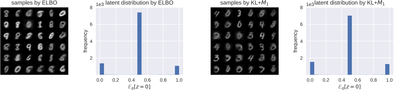
If a given dataset requires only a few latent codes to describe, then the redundant latent space will have their posteriors match the prior. In Figure 11, we see that is the case when the VAE model is trained by ELBO or +. The histograms show the distributions of the posterior means. Many of the latent dimensions have mean 0.5, suggesting that these dimensions do not encode meaning information about the data.
| MNIST | Fashion | CelebA | ||||
| Method | FID | KID | FID | KID | FID | KID |
| Baseline | ||||||
| VAE | 5.58 | 96.8 | 4.89 | 81.1 | 55.4 | 56.9 |
| Variational | ||||||
| + | 5.24 | 90.2 | 4.63 | 73.5 | 54.6 | 56.1 |
| + | 2.93 | 54.7 | 4.86 | 79.4 | 59.2 | 58.6 |
| + | 5.81 | 99.8 | 4.77 | 76.0 | 54.3 | 55.1 |
| + | 2.88 | 44.3 | 3.65 | 52.2 | 60.4 | 60.0 |
| + | 12.6 | 264 | 10.7 | 205 | 208 | 226 |
| + | 8.70 | 177 | 28.6 | 637 | 203 | 196 |
B.3 Generated samples
The generated samples in Figures 12, 13 and 14 are drawn from models with ConvNets, and Figures 15, 16 and 17 with ResNets.


