Prograde and Retrograde Gas Flow around Disk-embedded Companions: Dependence on Eccentricity, Mass and Disk Properties
Abstract
We apply 3D hydrodynamical simulations to study the rotational aspect of gas flow patterns around eccentric companions embedded in an accretion disk around its primary host. We sample a wide range of companion mass ratio and disk aspect ratio , and confirm a generic transition from prograde (steady tidal interaction dominated) to retrograde (background Keplerian shear dominated) circum-companion flow when orbital eccentricity exceeds a critical value . We find for sub-thermal companions while for super-thermal companions, and propose an empirical formula to unify the two scenarios. Our results also suggest that is insensitive to modest levels of turbulence, modeled in the form of a kinematic viscosity term. In the context of stellar-mass Black Holes (sBHs) embedded in AGN accretion disks, the bifurcation of their circum-stellar disk (CSD) rotation suggest the formation of a population of nearly anti-aligned sBHs, whose relevance to low spin gravitational wave (GW) events can be probed in more details with future population models of sBH evolution in AGN disks, making use of our quantitative scaling for ; In the context of circum-planetary disks (CPDs), our results suggest the possibility of forming retrograde satellites in-situ in retrograde CPDs around eccentric planets.
I Introduction
When a low-mass secondary companion is embedded in the accretion disk around its primary host, a circum-companion disk may form within the companion’s Bondi or Hills radius. In the context of protoplanetary disks (PPDs), extensive simulations establish the formation of prograde circum-planetary disks (CPDs) around embedded planets on circular orbits (Korycansky & Papaloizou 1996; Lubow et al. 1999; Tanigawa & Watanabe 2002; Machida et al. 2008; Tanigawa et al. 2012; Ormel 2013; Ormel et al. 2015a; Ormel et al. 2015b; Szulágyi et al. 2014; Fung et al. 2015; Li et al. 2021a; Szulágyi et al. 2022; Maeda et al. 2022). That is, the circum-planetary rotation will be aligned with the global disk rotation, maintained by steady tidal perturbation and existence of horseshoe streamlines in co-rotation, in competition against an effectively retrograde Keplerian background shear. Recently, it is suggested in Bailey et al. 2021; Li et al. 2022 that with moderate orbital eccentricity (, where is the disk aspect ratio), the horseshoe flows are disrupted, and the background shear will dominate to produce a retrograde CPD flow. Gas accretion from a retrograde CPD can strongly influence the evolution of planetary spins through gas accretion (Batygin 2018; Ginzburg & Chiang 2020), and may also be relevant to formation of retrograde satellites.
Moreover, it is emphasized in Li et al. 2022 that such phenomenon is generic for stellar-mass Black Holes (sBHs) embedded in active galactic nucleus (AGN) accretion disks surrounding supermassive Black Holes (SMBHs), since it’s not uncommon for these sBHs to obtain eccentricities due to birth kicks (Lousto et al. 2012) and other dynamical interactions (Zhang et al. 2014; Secunda et al. 2019; Secunda et al. 2020). Bifurcation of spin evolution of sBHs accreting from prograde/retrograde circum-stellar disks (CSDs, analogous to CPDs) produce mis-aligned (or nearly anti-aligned) sBH populations, the coalescence of which can produce low effective spin events consistent with most LIGO/Virgo detections (The LIGO Scientific Collaboration et al. 2021), which reinforces the idea that AGNs could be promising sites for observable sBH merger gravitational wave events (McKernan et al. 2012; McKernan et al. 2014; Bartos et al. 2017; Stone et al. 2017; Leigh et al. 2018; Tagawa et al. 2020a; Tagawa et al. 2020b; Davies & Lin 2020; Li et al. 2021b; Li et al. 2021c; Li & Lai 2022). Here the effective spin parameter is the mass-weighted-average of the sBH (merger components) spins projected along the binary orbital angular momentum, whose distribution can help constrain compact-object merger pathways (Gerosa et al. 2018; Bavera et al. 2020; Wang et al. 2021; Tagawa et al. 2021, e.g.,).
To determine the influence of orbital eccentricity on the spin evolution of sBH populations and subsequent merger signals in details, quantitative prescriptions for CSD flow transition should be incorporated into population synthesis models of sBH evolution in AGN disks. While Li et al. 2022 demonstrates a generic transition eccentricity between prograde and retrograde CSDs dependent on companion mass ratios and disk properties, their 2D simulations do not cover sufficient parameter space to conclude a comprehensive scaling for . In this Letter, we follow Bailey et al. 2021 and perform extensive 3D simulations of companion-disk interaction to determine the detailed dependence of on companion mass and disk properties. The simulation setup is laid out in §II, we analyze our results in §III and discuss the implication of our concluded formula in §IV.
II Numerical Setup
We use Athena++ to solve hydrodynamic equations in a spherical coordinate system () rotating at the Keplerian frequency , following the setup of Bailey et al. 2021. A companion of mass with semi-major axis and eccentricity is set to orbit around a host mass , where is the mass ratio. Therefore, the location of the companion embedded in the midplane are described with the epicyclic approximation:
| (1) | ||||
The code unit system is . The sound speed is a fixed value such that the disk is globally isothermal, where is the Keplerian velocity of the guiding center and is the aspect ratio at . The aspect ratio and the disk scale height are functions of distance
| (2) |
but within a small radial range centered at , they are going to be very close to , . We explore a range of in our simulations. The initial axi-symmetric hydrostatic equilibrium profile is set up according to Bailey et al. 2021, which gives roughly a power-law radial distribution for the midplane density , and a vertically integrated surface density . A fiducial was chosen but only acts as a normalization constant since we do not include active self-gravity or gas feedback on the companion. The companion potential term was increased gradually over two orbits (“ramped-up”) to the designated value.
We define the following relevant length scales to facilitate our analysis. The Bondi radius
| (3) |
arises as the natural length scale comparing the companion gravity to the thermal state of the nebular gas. The Hill radius
| (4) |
on the other hand, is the natural length scale comparing the strength of companion gravity the host’s tidal gravity in the corotating frame.
The thermal mass ratio is defined as
| (5) |
Such that low mass companions lie in the sub-thermal regime where represented by where moderate mass companions lie in the super-thermal regime where represented by . Additionally, considering the companion’s extra epicyclic velocity about its guiding center , the effective Bondi radius is reduced to the Bondi-Hoyle-Lyttleton radius
| (6) |
which depicts more accurately an impact parameter of the circum-companion disk (hereafter generally referred to as CSD) in either all sub-thermal cases or super-thermal cases where is sufficiently large. The softening scale of for companion potential is deliberately chosen to resolve CSD flow patterns for a companion that has sufficiently small physical/atmospheric radius compared to , most applicable to sBHs. This softening is also much smaller than the Hill radius, even for our largest super-thermal companions (, such that is no smaller than 0.15). We also restrict our simulations to to ensure in super-thermal cases even if . We also constrain the absolute eccentricity to be , beyond which the companion is hard to maintain such eccentricity long-term and the epicycle approximation may be inaccurate . All models are run for 40 orbits, which is enough time for flow fields to reach quasi-steady or quasi-periodic state.
II.1 Boundaries and Resolution
Identical to Bailey et al. 2021, we cover the computational domain with a root grid of , such that the root cell around has a width of . The azimuthal and polar spacings are linear and the radial spacing is logarithmic. We also apply fixed radial boundaries, periodic azimuthal boundaries, and reflecting polar boundaries.
To properly resolve the CSD region, we apply Adaptive Mesh Refinement (AMR) and impose maximum-resolution over a whole volume within a distance of from the companion location. This distance ranges from 2 softening lengths for the largest to 40 softening lengths for the smallest choice of . Within this region of maximum-resolution, we add 7 layers of refinement on top of the root grid such that for the smallest cell width is guaranteed for , and the smoothing length can be resolved. Away from the companion, the resolution adjusts itself to relax gradually outside the region of maximum-resolution towards the default background resolution.
III Results
III.1 Fiducial Cases
Since we apply lower central resolution and larger softening than the simulations in Bailey et al. 2021, we are able to run each simulation much quicker. For each given companion mass ratio and characteristic scale height , we are able to sample a number of eccentricities to determine the transition point to high accuracy. For example, it is reported in Bailey et al. 2021 that for , the CSD flow should be prograde for but retrograde for , while we are able to identify for a similar parameter . Such mass ratio is applicable to Neptunes around solar-mass planets or sBHs around low mass SMBHs.
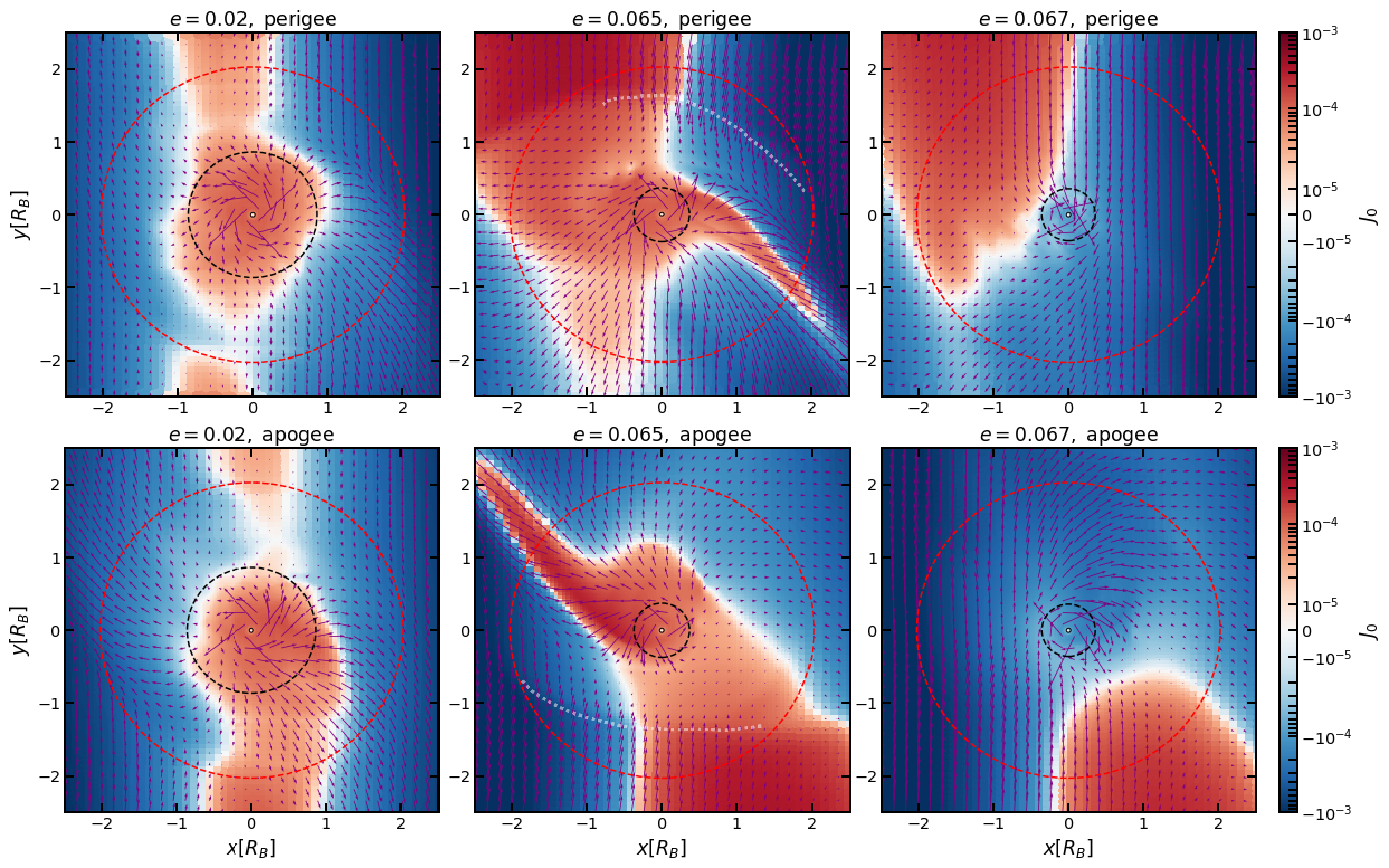
We plot in Figure 1 the midplane specific angular momentum with respect to the companion for the marginal cases (prograde CSD, upper panel) and (retrograde CSD, lower panel), analogous to Figure 2 of Li et al. 2022. The left panels are at perigee and right panels are at apogee. As in Bailey et al. 2021, we make use of another unsubscripted coordinate system or centered on the companion to discuss the rotational aspect of the CSD flow. In this coordinate system, is the product of companion-centric distance , and the gas velocity component along the companion-centric azimuth . Red color is prograde motion and blue is retrograde. The distances in Figure 1 are measured in and the central solid black circles denote . Additionally, we plot with black dashed circle and with red dashed circles. At large radial locations from the companion, the Keplerian shear background is always retrograde. Within , gas is subject to the companion’s gravity and its rotation always forms a CSD, regardless of the sign of the specific angular momentum. We plot in Figure 2 the -averaged distribution (in other words, rotation curves) up to a much smaller scale within compared to Figure 1, which confirm that at both perigee and apogee, the prograde/retrograde rotations converge to Keplerian at small enough radii. The Keplerian rotation deviates slightly from a power law at small due to the prescribed gravitational softening. For increasing eccentricity, the convergence towards axi-symmetric Keplerian flow (or towards a CSD structure) happens at smaller radii since realistic impact parameter continues to decrease. The rotation curves at other orbital phases show similar results.
We can compare our fiducial results with 2D simulations in Li et al. 2022 for a similar parameter and . Our transition eccentricity is significantly larger than their value around , and the morphology of flow pattern is notably different. In Li et al. 2022, the CSD’s transition from classical prograde to retrograde is directly associated with the receding of horseshoe structures from the CSD region at , above which the CSD flow becomes directly connected with retrograde background. For even larger supersonic eccentricity , a strong prograde head-wind region appears at the upper left/lower right corner of the planet at perigee/apogee adjacent to the retrograde CSD, a feature of the shear background flow due to orbital eccentricity, which penetrates deeper into and introduce more fluctuations in the CSD rotation curve as continues to increase.
While our result for retrograde CSDs at is similar to the 2D high eccentricity limit (e.g. ), prograde CSDs in 3D formed through tidal interaction seem to be much more resilient to disturbances, such that it could still preserve its rotation for eccentricities up to even when the classical horseshoe flow pattern has been disrupted. Indeed, even in the limit of negligible eccentricity, a major feature of 3D circum-companion flow structure compared to 2D is that the horseshoe region is narrower and the radial velocity of gas making U-turn is much smaller, as shown in Figure 3 of Ormel et al. 2015b. This is why even for small eccentricity (left panel, Figure 1), the red band with prograde motion at large azimuths from the planet, representing horseshoe streamlines with notable radial motion, is quite narrow compared to 2D simulations.
Despite having a more significantly prograde horseshoe region at low , above the CSD turns abruptly from prograde to retrograde in 2D. However in 3D, we found that the flow pattern similar to case can be maintained up to . At even larger eccentricity, the classical horseshoe structure becomes completely replaced by the fore-mentioned headwind region, e.g. in the marginally prograde case (middle panel, Figure 1). Due to the super-sonic epicyclic velocity, a shock front (sketched out with faint white lines) appears and barricades a prograde CSD against the disk background, which it continuously rams into. For even larger (right panel, Figure 1), the shock front finally breaks down and the background overcomes the CSD to mould it into a retrograde flow.
To summarize different eccentricity regimes, at the CSD is mildly perturbed and shows sign of detaching from a horseshoe region that’s narrower compared to 2D simulations, at the horseshoe flow pattern disappears, while a shock front appears between the CSD and the background disk, but the prograde rotation is still maintained. At the CSD becomes retrograde where the midplane flow pattern is similar to 2D retrograde cases.
Apart from the appearance of the parameter space where companions could maintain prograde CSDs for slightly super-sonic eccentricities, the generic transition to retrograde in 2D and 3D is qualitatively similar. Namely, the CSD flow changes from tidal effect dominated to shear background dominated at large , albeit in 3D that the transition is better marked by the fading of a shock front rather than horseshoe patterns. Our finding implies that the retrograde criterion is connected to the ability of background retrograde flow to penetrate into the shock fronts (observed in prograde cases) and overcome the CSD. We try to directly associate this with the size of CSDs in §III.2.
III.2 The Parameter Survey
After running resolution convergence tests with and an extra layer of central refinement for the fiducial case (resolution of Bailey et al. 2021), we found an identical result , with flow patterns the same as §III.1 for and . We conclude that it’s adequate to apply our default resolution for large parameter surveys. In our full survey, we cover three scale heights and extend to larger . The low scale height especially applies to AGN disks (Sirko & Goodman 2003; Levin 2007). The companion mass can be scaled to planetary/SBH masses of
| (7) |
We summarize the results of our survey on Figure 3. The transition eccentricity (with error-bars) is plotted against in solid lines. Different colors correspond to different , and each column of symbols represent a set of simulations with fixed but varying : squares represent prograde final states for the CSDs at while circles represent prograde ones at .
We start from () where the softening length is narrowly resolved by cells, then simulate progressively larger cases at each . For sub-thermal companions with , we found a generic insensitive to , as hypothesized by Bailey et al. 2021 (super-sonic eccentric velocity leads to retrograde flow). However, for super-thermal companions with , the scaling steepens. This dependence of on the companion mass is quite significant for our largest masses at .
A natural way to account for the steepening of the scaling is to interpret the super-sonic eccentricity retrograde flow criterion as a requirement for the size of BHL radius with respect to the circular-orbit impact parameter, e.g. the Bondi radius in the sub-thermal limit:
| (8) |
which means that when eccentricity is large and the epicyclic head-wind is strong enough, will be small enough, such that the CSD’s characteristic bounded angular momentum can no longer maintain a shock front and it becomes significantly perturbed by the background retrograde flow, as discussed in §III.1.
To generalize to super-thermal companions, we express the reference impact parameter by and obtain
| (9) |
which translates into
| (10) |
so the transition eccentricity can be expressed as
| (11) |
or explicitly
| (12) |
This formula for the retrograde criterion naturally gives us a transition of scaling from towards at . Note that implies that always holds at even for super-thermal companions.
In Figure 4 we plot the normalized eccentricity against for all our and compare them with Equation 12, assuming . This is chosen to fit with the flat scaling on the sub-thermal side, which appears to be quite universal for all values of ; The super-thermal side of our analytical scaling fits quite well with cases. The scaling produced in our simulation starts to rise from the flat profile only after but also quickly catches up towards scaling afterwards, possibly because shocks are stronger for low sound speed in a non-linear way and a prograde CSD is more easily overcome by shock for certain companion masses.
It is possible that the scaling might break down for even larger mass regime, which is beyond the scope of this study. Nevertheless, we note that if we extend this scaling to binaries of comparable mass , the critical eccentricity would reach order-unity, consistent with circum-binary simulations (Muñoz et al. 2019; D’Orazio & Duffell 2021, e.g.), in which circum-single disks around binary components should always be prograde for arbitrarily eccentricity.
III.3 Effect of Viscosity: Application to AGN Context
Albeit both simulation and observation suggest that planet-forming mid-planes of PPDs have low turbulent viscosities (Bai & Stone 2013; Flaherty et al. 2017; Flaherty et al. 2020), AGN disks can be highly turbulent with magneto-rotational instability (MRI) (Balbus & Hawley 1998) and gravitational instability (GI) (Gammie 2001) providing effective turbulence parameter (Shakura & Sunyaev 1973) up to (Goodman 2003). To briefly explore how turbulent viscosity affect inviscid flow structures, we run additional tests based on the model (corresponding to in an AGN context) focusing on determining the transition eccentricities around , with constant kinetic viscosity in code units to approximate a turbulence parameter close to the companion. We found that with a moderate viscosity, is reduced slightly to from . The distributions within for these marginal cases with are presented in Figure 5. They are all averaged over 10 perigees and the apogee distribution is quite analogous.

In the inviscid simulations (upper panels, Figure 5), the and flow pattern is similar to to the fiducial case at . Although is slightly super-thermal in the sense that and that in the circular-orbit limit case the CSD size should be constrained by instead of (Martin & Lubow 2011), from the summary in §III.2 we know that at around we always have , therefore the extent of CSD rotation is still mainly constrained by the BHL radius rather than . The marginally retrograde CSD structure at is also similar to the fiducial case at accompanied with the fading of a shock front, albeit not as abrupt as in Figure 1. The shock completely disappears around closer to the given by Equation 12, which may be relevant to deviation of the curve in Figure 4 from analytical prescription, in the sense that while Equation 12 can indeed reflect the point where shock front is overcome by strong headwind, for small the CSD rotation can become dominated by background flow before the complete disappearance of the shock.
In the simulations (lower panels, Figure 5) the transition is quite similar, with producing prograde and both and 0.014 producing retrograde CSDs. The slight reduction of is probably due to shock fronts being harder to maintain in the presence of viscosity.
Based on this additional set of simulations, we conclude that is not sensitive to viscosity up to moderate values of , and the main cause for being generally much larger than Li et al. 2022 should be due to 2D/3D geometry, instead of their simulations having . Nevertheless, the kinematic viscosity term in laminar fluid equations is only to approximate the vortensity diffusion and angular momentum transfer effect of realistic turbulence (Baruteau & Lin 2010), which is useful for low turbulence level but could fail to capture important effects from velocity/density fluctuations in the case of strong turbulence with . Furthermore, magnetic fields may provide large scale coupling between the CSDs and the background flow, leading to different results from disks (Zhu et al. 2013). To explore such levels of turbulence, it is worth performing simulations of companions embedded in realistic MRI or GI environments.
IV Conclusions
We confirm the retrograde circum-stellar flow criterion for eccentric sub-thermal disk-embedded companions proposed in Bailey et al. 2021; Li et al. 2022, and extend to super-thermal companions. The dependence of transition eccentricity on mass ratio and disk scale height can be incorporated into the empirical formula Equation 12, for which we have offered some analytical understanding. Our results also suggest that is relatively insensitive to viscosity. The results have several implications.
In terms of CPDs, retrograde rotation may lead to in-situ formation of retrograde satellites, as an alternative channel from dynamical capture, e.g. the case of Triton (McKinnon & Leith 1995). Dynamical events such as mergers and ejections in multiple planets can excite eccentricity of planets to typically 0.1 (Zhou et al. 2007; Ida & Lin 2010; Ida et al. 2013; Bitsch et al. 2020). In the presence of a gaseous disk, large eccentricities are quickly damped towards a residual value if low-mass planets form mean-motion resonance chains through migration (Zhang et al. 2014; Liu et al. 2015). Therefore, it is still likely that moderate eccentricity and retrograde CPDs could be maintained for a considerable fraction of PPD lifetimes, which is adequate for significant in-situ pebble growth in CPDs (Drażkowska & Szulágyi 2018; Szulágyi et al. 2018). Considering in PPDs similar to the early outer solar nebula (Chiang & Youdin 2010), for Jupiter mass and for Saturn mass so their is large. Therefore it may be more likely to form retrograde CPDs around sub-thermal, Neptune-mass objects. Subsequent works may explore solid accretion in retrograde CPDs, but we generally remark that in-situ formation of retrograde satellites should prefer multi-planet systems where planetary eccentricities are easier to maintain, and may be more likely around Neptune-mass planets.
For sBHs embedded in AGN scenario, the disk scale height is typically (Sirko & Goodman 2003; Nayakshin & Cuadra 2007; Levin 2007), therefore the normalized mass ratio is nearly always sub-thermal () for sBH mass , and SMBH mass in the range of . Similar to the planetary context, multiple sBHs can also form resonance chains through migration and maintain from their mutual dynamical interaction (Secunda et al. 2019; Secunda et al. 2020). If their spin evolution is coupled with the rotation of their surrounding CSDs, the sBHs will be spin up to critical rotation on their Eddington mass accretion timescales, with circular ones being spun up in the prograde direction, and eccentric ones being spun up in the retrograde direction, as discussed in some detail by Li et al. 2022. This leads to formation of a population of misaligned sBHs spun up by prograde and retrograde CSDs, depending on dispersion in their initial eccentricity distribution. Merging of mis-aligned pairs of sBHs would contribute to subsequent low GW events. Our quantitative criterion can be readily incorporated into sBH population synthesis models (Tagawa et al. 2020b; Tagawa et al. 2020a; McKernan et al. 2022) to study the detailed influence of eccentricity distribution on the GW wave signal properties.
Y.X.C would like to thank Douglas Lin and Ya-Ping Li for helpful discussions. We also acknowledge computational resources provided by the high-performance computer center at Princeton University, which is jointly supported by the Princeton Institute for Computational Science and Engineering (PICSciE) and the Princeton University Office of Information Technology.
References
- Bai & Stone (2013) Bai, X.-N., & Stone, J. M. 2013, ApJ, 769, 76, doi: 10.1088/0004-637X/769/1/76
- Bailey et al. (2021) Bailey, A., Stone, J. M., & Fung, J. 2021, ApJ, 915, 113, doi: 10.3847/1538-4357/ac033b
- Balbus & Hawley (1998) Balbus, S. A., & Hawley, J. F. 1998, Reviews of Modern Physics, 70, 1, doi: 10.1103/RevModPhys.70.1
- Bartos et al. (2017) Bartos, I., Kocsis, B., Haiman, Z., & Márka, S. 2017, ApJ, 835, 165, doi: 10.3847/1538-4357/835/2/165
- Baruteau & Lin (2010) Baruteau, C., & Lin, D. N. C. 2010, ApJ, 709, 759, doi: 10.1088/0004-637X/709/2/759
- Batygin (2018) Batygin, K. 2018, AJ, 155, 178, doi: 10.3847/1538-3881/aab54e
- Bavera et al. (2020) Bavera, S. S., Fragos, T., Qin, Y., et al. 2020, A&A, 635, A97, doi: 10.1051/0004-6361/201936204
- Bitsch et al. (2020) Bitsch, B., Trifonov, T., & Izidoro, A. 2020, A&A, 643, A66, doi: 10.1051/0004-6361/202038856
- Chiang & Youdin (2010) Chiang, E., & Youdin, A. N. 2010, Annual Review of Earth and Planetary Sciences, 38, 493, doi: 10.1146/annurev-earth-040809-152513
- Davies & Lin (2020) Davies, M. B., & Lin, D. N. C. 2020, MNRAS, 498, 3452, doi: 10.1093/mnras/staa2590
- D’Orazio & Duffell (2021) D’Orazio, D. J., & Duffell, P. C. 2021, ApJ, 914, L21, doi: 10.3847/2041-8213/ac0621
- Drażkowska & Szulágyi (2018) Drażkowska, J., & Szulágyi, J. 2018, ApJ, 866, 142, doi: 10.3847/1538-4357/aae0fd
- Flaherty et al. (2020) Flaherty, K., Hughes, A. M., Simon, J. B., et al. 2020, ApJ, 895, 109, doi: 10.3847/1538-4357/ab8cc5
- Flaherty et al. (2017) Flaherty, K. M., Hughes, A. M., Rose, S. C., et al. 2017, ApJ, 843, 150, doi: 10.3847/1538-4357/aa79f9
- Fung et al. (2015) Fung, J., Artymowicz, P., & Wu, Y. 2015, ApJ, 811, 101, doi: 10.1088/0004-637X/811/2/101
- Gammie (2001) Gammie, C. F. 2001, ApJ, 553, 174, doi: 10.1086/320631
- Gerosa et al. (2018) Gerosa, D., Berti, E., O’Shaughnessy, R., et al. 2018, Phys. Rev. D, 98, 084036, doi: 10.1103/PhysRevD.98.084036
- Ginzburg & Chiang (2020) Ginzburg, S., & Chiang, E. 2020, MNRAS, 491, L34, doi: 10.1093/mnrasl/slz164
- Goodman (2003) Goodman, J. 2003, MNRAS, 339, 937, doi: 10.1046/j.1365-8711.2003.06241.x
- Ida & Lin (2010) Ida, S., & Lin, D. N. C. 2010, ApJ, 719, 810, doi: 10.1088/0004-637X/719/1/810
- Ida et al. (2013) Ida, S., Lin, D. N. C., & Nagasawa, M. 2013, ApJ, 775, 42, doi: 10.1088/0004-637X/775/1/42
- Korycansky & Papaloizou (1996) Korycansky, D. G., & Papaloizou, J. C. B. 1996, ApJS, 105, 181, doi: 10.1086/192311
- Leigh et al. (2018) Leigh, N. W. C., Geller, A. M., McKernan, B., et al. 2018, MNRAS, 474, 5672, doi: 10.1093/mnras/stx3134
- Levin (2007) Levin, Y. 2007, MNRAS, 374, 515, doi: 10.1111/j.1365-2966.2006.11155.x
- Li & Lai (2022) Li, R., & Lai, D. 2022, arXiv e-prints, arXiv:2202.07633. https://arxiv.org/abs/2202.07633
- Li et al. (2022) Li, Y.-P., Chen, Y.-X., Lin, D. N. C., & Wang, Z. 2022, ApJ, 928, L1, doi: 10.3847/2041-8213/ac5b61
- Li et al. (2021a) Li, Y.-P., Chen, Y.-X., Lin, D. N. C., & Zhang, X. 2021a, ApJ, 906, 52, doi: 10.3847/1538-4357/abc883
- Li et al. (2021b) Li, Y.-P., Dempsey, A. M., Li, H., Li, S., & Li, J. 2021b, arXiv e-prints, arXiv:2112.11057. https://arxiv.org/abs/2112.11057
- Li et al. (2021c) Li, Y.-P., Dempsey, A. M., Li, S., Li, H., & Li, J. 2021c, ApJ, 911, 124, doi: 10.3847/1538-4357/abed48
- Liu et al. (2015) Liu, B., Zhang, X., Lin, D. N. C., & Aarseth, S. J. 2015, ApJ, 798, 62, doi: 10.1088/0004-637X/798/1/62
- Lousto et al. (2012) Lousto, C. O., Zlochower, Y., Dotti, M., & Volonteri, M. 2012, Phys. Rev. D, 85, 084015, doi: 10.1103/PhysRevD.85.084015
- Lubow et al. (1999) Lubow, S. H., Seibert, M., & Artymowicz, P. 1999, ApJ, 526, 1001, doi: 10.1086/308045
- Machida et al. (2008) Machida, M. N., Kokubo, E., Inutsuka, S.-i., & Matsumoto, T. 2008, ApJ, 685, 1220, doi: 10.1086/590421
- Maeda et al. (2022) Maeda, N., Ohtsuki, K., Tanigawa, T., Machida, M. N., & Suetsugu, R. 2022, arXiv e-prints, arXiv:2207.03664. https://arxiv.org/abs/2207.03664
- Martin & Lubow (2011) Martin, R. G., & Lubow, S. H. 2011, MNRAS, 413, 1447, doi: 10.1111/j.1365-2966.2011.18228.x
- McKernan et al. (2022) McKernan, B., Ford, K. E. S., Callister, T., et al. 2022, MNRAS, 514, 3886, doi: 10.1093/mnras/stac1570
- McKernan et al. (2014) McKernan, B., Ford, K. E. S., Kocsis, B., Lyra, W., & Winter, L. M. 2014, MNRAS, 441, 900, doi: 10.1093/mnras/stu553
- McKernan et al. (2012) McKernan, B., Ford, K. E. S., Lyra, W., & Perets, H. B. 2012, MNRAS, 425, 460, doi: 10.1111/j.1365-2966.2012.21486.x
- McKinnon & Leith (1995) McKinnon, W. B., & Leith, A. C. 1995, Icarus, 118, 392, doi: 10.1006/icar.1995.1199
- Muñoz et al. (2019) Muñoz, D. J., Miranda, R., & Lai, D. 2019, ApJ, 871, 84, doi: 10.3847/1538-4357/aaf867
- Nayakshin & Cuadra (2007) Nayakshin, S., & Cuadra, J. 2007, A&A, 465, 119, doi: 10.1051/0004-6361:20065541
- Ormel (2013) Ormel, C. W. 2013, MNRAS, 428, 3526, doi: 10.1093/mnras/sts289
- Ormel et al. (2015a) Ormel, C. W., Kuiper, R., & Shi, J.-M. 2015a, MNRAS, 446, 1026, doi: 10.1093/mnras/stu2101
- Ormel et al. (2015b) Ormel, C. W., Shi, J.-M., & Kuiper, R. 2015b, MNRAS, 447, 3512, doi: 10.1093/mnras/stu2704
- Secunda et al. (2019) Secunda, A., Bellovary, J., Mac Low, M.-M., et al. 2019, ApJ, 878, 85, doi: 10.3847/1538-4357/ab20ca
- Secunda et al. (2020) —. 2020, ApJ, 903, 133, doi: 10.3847/1538-4357/abbc1d
- Shakura & Sunyaev (1973) Shakura, N. I., & Sunyaev, R. A. 1973, A&A, 500, 33
- Sirko & Goodman (2003) Sirko, E., & Goodman, J. 2003, MNRAS, 341, 501, doi: 10.1046/j.1365-8711.2003.06431.x
- Stone et al. (2017) Stone, N. C., Metzger, B. D., & Haiman, Z. 2017, MNRAS, 464, 946, doi: 10.1093/mnras/stw2260
- Szulágyi et al. (2022) Szulágyi, J., Binkert, F., & Surville, C. 2022, ApJ, 924, 1, doi: 10.3847/1538-4357/ac32d1
- Szulágyi et al. (2018) Szulágyi, J., Cilibrasi, M., & Mayer, L. 2018, ApJ, 868, L13, doi: 10.3847/2041-8213/aaeed6
- Szulágyi et al. (2014) Szulágyi, J., Morbidelli, A., Crida, A., & Masset, F. 2014, ApJ, 782, 65, doi: 10.1088/0004-637X/782/2/65
- Tagawa et al. (2020a) Tagawa, H., Haiman, Z., Bartos, I., & Kocsis, B. 2020a, ApJ, 899, 26, doi: 10.3847/1538-4357/aba2cc
- Tagawa et al. (2021) Tagawa, H., Haiman, Z., Bartos, I., Kocsis, B., & Omukai, K. 2021, MNRAS, 507, 3362, doi: 10.1093/mnras/stab2315
- Tagawa et al. (2020b) Tagawa, H., Haiman, Z., & Kocsis, B. 2020b, ApJ, 898, 25, doi: 10.3847/1538-4357/ab9b8c
- Tanigawa et al. (2012) Tanigawa, T., Ohtsuki, K., & Machida, M. N. 2012, ApJ, 747, 47, doi: 10.1088/0004-637X/747/1/47
- Tanigawa & Watanabe (2002) Tanigawa, T., & Watanabe, S.-i. 2002, ApJ, 580, 506, doi: 10.1086/343069
- The LIGO Scientific Collaboration et al. (2021) The LIGO Scientific Collaboration, the Virgo Collaboration, the KAGRA Collaboration, et al. 2021, arXiv e-prints, arXiv:2111.03606. https://arxiv.org/abs/2111.03606
- Wang et al. (2021) Wang, Y.-H., McKernan, B., Ford, S., et al. 2021, ApJ, 923, L23, doi: 10.3847/2041-8213/ac400a
- Zhang et al. (2014) Zhang, X., Liu, B., Lin, D. N. C., & Li, H. 2014, ApJ, 797, 20, doi: 10.1088/0004-637X/797/1/20
- Zhou et al. (2007) Zhou, J.-L., Lin, D. N. C., & Sun, Y.-S. 2007, ApJ, 666, 423, doi: 10.1086/519918
- Zhu et al. (2013) Zhu, Z., Stone, J. M., & Rafikov, R. R. 2013, ApJ, 768, 143, doi: 10.1088/0004-637X/768/2/143