Unfocused notes on the Markoff equation and T-Singularities

Markus Perling

Abstract.

We consider minimal resolutions of the singularities for weighted projective planes of type $\mathbb{P}(e^{2},f^{2},g^{2})$ , where $e,f,g$ satisfy the Markoff equation $e^{2}+f^{2}+g^{2}=3efg$ . We give a complete classification of such resolutions in terms of continued fractions similar to classical work of Frobenius. In particular, we investigate the behaviour of resolutions under mutations and describe a Cantor set emerging as limits of continued fractions.

2020 Mathematics Subject Classification

Primary: 14J17, 11J06; Secondary: 28A78, 28A80, 14F08

1. Introduction

The main aim of these notes is to describe the minimal resolutions of singularities for weighted projective planes $\mathbb{P}(e^{2},f^{2},g^{2})$ , where $e,f,g$ are integral solutions of the Markoff equation:

e^{2}+f^{2}+g^{2}=3efg.

It has been observed in [HP10] that these singularities are T-singularities in the sense of Wahl [Wah81]. Such singularities have been connected to exceptional vector bundles on rational surfaces by results of Hacking-Prokhorov [HP10] and Hacking [Hac13]. This aspect has also been investigated in our earlier work [HP08], [Per18]. We think that the complete understanding of these resolutions and the fractal structure emerging via the associated Markoff tree are of independent interest, but our hope is that this also may lead to further insights into the global structure of exceptional collections.

Consider a T-singularity of type $\frac{1}{n^{2}}(1,nk-1)$ , i.e. a cyclic quotient singularity of order $n^{2}$ with weights $1,nk-1$ . The minimal resolution of such a singularity can be desribed via Hirzebruch-Jung continued fractions $\llbracket a_{1},\dots,a_{t}\rrbracket=a_{1}-1/(a_{2}-1/(a_{3}-\cdots(a_{t-1}-1/a_{t})\cdots))$ . These continued fractions have been classified for T-singularities in [KS88] (see also Section 6). Our first basic tool will be a simplified representation of these Hirzebruch-Jung continued fractions in terms of integer sequences $c_{1},\dots,c_{s}$ (see Section 6), which is based on the Kollár–Shepherd-Barron classification. It turns out that the $c_{i}$ can be recovered from the regular continued fraction expansion $n^{2}/(nk-1)=[c_{s}+1,c_{s-1},\dots,c_{2},c_{1}+x,c_{1}+2-x,c_{2},\dots,c_{s-1},c_{s}+1]$ , where $x=2$ if $s$ is even and $x=0$ if $s$ is odd (Theorem 7.8).

Now, for any Markoff triple $(e,f,g)$ with $1<e,f<g$ , $\mathbb{P}(e^{2},f^{2},g^{2})$ has the three T-singularities $\frac{1}{e^{2}}(1,ew_{e}-1)$ , $\frac{1}{f^{2}}(1,fw_{f}-1)$ and $\frac{1}{g^{2}}(1,gw_{g}-1)$ , respectively, where we call $w_{e},w_{f},w_{g}$ the T-weights of this triple. When passing from one Markoff triple to the next, say $(e,g,E)$ with $E=3fg-e$ , we will show in Section 7 how to construct the continued fraction of $E^{2}/(Ew_{E}-1)$ from those of $\frac{1}{e^{2}}(1,ew_{e}-1)$ , $\frac{1}{f^{2}}(1,fw_{f}-1)$ and $\frac{1}{g^{2}}(1,gw_{g}-1)$ , respectively, and thereby obtain a complete classification of the minimal resolutions of T-singularities associated to Markoff triples in terms of their mutations along the Markoff tree.

A strongly related question is the distribution of quotients $g/w_{g}\approx g^{2}/(gw_{g}-1)$ and whether limits of such quotients exists when mutating Markoff triples downward paths in the Markoff tree. This is very closely related to classical work by Frobenius [Fro68]. In loc. cit., Frobenius derives a complete description of continued fraction expansions of quotients $g/r_{g}$ , where $r_{g}$ is associated to a triple that contains $g$ such that $r_{g}^{2}\equiv-1\mod g$ . Using Frobenius’ description, it is straightforward to see that limits $\lim_{i\rightarrow\infty}r_{g_{i}}/g_{i}$ exist, for any sequence $g_{i}$ that follows a path downward the Markoff tree (Proposition 4.3). It turns out that the set of these limit points forms a Cantor set. We will show that this set has measure and Hausdorff dimension zero (Theorems 4.9 and 4.12). Moreover, we will characterize this Cantor set by its natural intervals and we will show that the boundary points of these intervals are quadratic numbers, which are explicitly described in Proposition 4.5.

The quotients $w_{g}/g$ are related to the $r_{g}/g$ simply by the affine transform $w_{g}/g=3r_{g}/g-1$ for every $g$ (Corollary 5.4). Therefore, their limit points via the Markoff tree exist as well and the resulting Cantor set is an affine transform of the one associated to the $r_{g}/g$ . Their dimension and measure therefore coincide (Theorem 7.11). The boundary points are quadratic as well and their explicit formulas and periodic continued fraction expansions are computed in Secton 7.

We point out that the quotients $r_{g}/g$ have shown up in earlier work as the slopes of exceptional vector bundles on $\mathbb{P}^{2}$ , see [Rud89], [DL85], and their fractal nature has already been observed in [DL85].

Overview. In Section 2 we fix some general conventions regarding the Markoff tree that we will follow for the rest of these notes. In Section 3, we collect all fundamental facts and computations related to Markoff triples that will be needed in the subsequent sections. This includes some well-known formulas, but also some new formulas for which we could not find any reference in the literature. Also, we review Frobenius’ results on continued fractions related to Markoff triples. In Section 4 we use the results of Section 3 to analyze the Cantor set that emerges from the quotients $r_{g}/g$ . In Section 5, we introduce T-weights and perform some calculations similar as in Section 3. In Section 6, we analyze the continued fraction expansions of T-singularities. We then apply these results in the final Section 7 in order to classify the minimal resolutions for T-singularities associated to the Markoff equation and to describe the Cantor set that emerges from the quotients $w_{g}/g$ .

In Appendix A we collect some basic facts about continued fractions and continuants that we will need throughout the text. In Appendix B we introduce a new class of polynomials related to T-singularities. These are not needed in the main body of these notes, but they may be of independent interest. In Appendix C, we collect some material that we need in order to deal with the Hausdorff dimension. In Appendix D, we display the first few levels of the Markoff tree, both only the maximal elements and the triples. We found it quite useful to be able to occasionally pinpoint a specific example and its location in the tree in one peek. Appendix E has a computer generated list of the first 300 Markoff numbers together with their weights and T-weights. If needed, the table can be extracted from this documents LaTeX source. In Appendix F we present some simplistic numerical experiments regarding the growth of Markoff numbers and the uniqueness conjecture.

2. The Markoff Tree

In this section we will state some general facts and fix our general conventions regarding the Markoff tree (we refer to [Aig13] for an overview). We are exclusively interested in positive integral solutions $(e,f,g)$ of the Markoff equation $e^{2}+f^{2}+g^{2}=3efg$ , which we will call Markoff triples. If for any given Markoff triple $(e,f,g)$ we denote $E=3fg-e$ , $F=3eg-f$ , and $G=3ef-g$ , then we obtain three more Markoff triples $(E,f,g)$ , $(e,F,g)$ , and $(e,f,G)$ . We call these substitutions mutations of the triple $(e,f,g)$ . By rearranging the formulas $3eg=f+F$ , $3fg=e+E$ , and $3ef=g+G$ , it becomes obvious that mutations are reversible. All Markoff triples can be obtained by mutation, starting from the fundamental solution $(1,1,1)$ . So we can consider the set of all Markoff triples as vertices of a trivalent acyclic graph whose edges are labeled by the mutations, where the fundamental solution is the natural root. By the symmetry of the Markoff equation, we have a natural action of the symmetric group $S_{3}$ on the set of Markoff triples. This action has an almost everywhere trivial stabilizer with exceptions $(1,1,1)$ and the permutations of $(1,2,1)$ . These triples, which are the only ones where $e,f,g$ are not pairwise distinct, are called singular solutions of the Markoff equation. All other Markoff triples are called regular. The set of regular Markoff triples up to permutation forms a binary tree, whose root is represented by the triple $(1,5,2)$ . Figure 1 shows the first few levels of this tree.

Figure 1. A part of the Markoff tree.

As in Figure 1, we will use from now on the convention that every regular Markoff triple will be represented by $(e,g,f)$ , such that $0<e,f<g$ . Because $g<E,F$ , mutation of $e$ or $f$ does mean that we descend downwards the Markoff tree, where we fix the direction as indicated in Figure 2.

Figure 2. Left and right mutation.

We will in call the triple $(e,F,g)$ the left mutation and $(g,E,f)$ the right mutation of $(e,f,g)$ , respectively. With this convention, if we go upwards by mutating $g$ , then we will either end up with the triple $(e,f,G)$ (if $e<f$ ) or $(G,e,f)$ (if $e>f$ ). By requiring that the root is represented by $(1,5,2)$ , the ordering of every representative is thus uniquely fixed. In particular, if we traverse any level below the root from left to right then we find that alternatingly $e<f$ or $e>f$ , with $1=e<f$ for the leftmost vertex and $e>f=2$ for the rightmost vertex.

It follows that, given a triple $(e,g,f)$ , then starting from this triple, there are precisely four branches where at least one of $e,f,g$ is preserved, as indicated by Figure 3.

Figure 3. How the elements in a Markoff triple propagate downwards.

The two outmost branches of the Markoff tree are of the form

(1,F_{2n+1},F_{2n-1})\text{ for }n\geq 2\quad\text{}\quad(P_{2n-1},P_{2n+1},2)\text{ for }n\geq 1,

where $F_{i}$ and $P_{i}$ denote the Fibonacci and Pell numbers. Note that $5=F_{5}=P_{3}$ . We call these the Fibonacci and Pell branches, respectively.

3. The Markoff tree and finite continued fractions à la Frobenius

In this section we give an expository overview around some aspects of Frobenius’ classical account [Fro68] on the Markoff equation which are related to finite continued fractions. We also refer to [Cas57, Chapter II], [CF89], [Aig13], [Reu19]. We will paraphrase some of the material to suit our needs and complement it by a few observations of our own which, though probably well-known to specialists, we couldn’t locate in the literature.

3.1. Weights and coweights

Denote $(e,g,f)$ a regular Markoff triple. Then we set:

	$\displaystyle r_{e}$	$\displaystyle:=\begin{cases}0&\text{ if }e=1,\\ f^{-1}g\bmod e&\text{ else},\end{cases}$
	$\displaystyle r_{f}$	$\displaystyle:=g^{-1}e\bmod f,$
	$\displaystyle r_{g}$	$\displaystyle:=e^{-1}f\bmod g.$

Note that the choice $r_{e}=0$ for $e=1$ is made for consistency, as we will see below. Then the Markoff equation implies that

r_{e}^{2}\equiv-1\bmod e\,\,(\text{for }e>1),\quad r_{f}^{2}\equiv-1\bmod f,\quad\text{ and }\quad r_{g}^{2}\equiv-1\bmod g.

We choose to call the triple $(r_{e},r_{g},r_{f})$ the weights associated to the triple $(e,g,f)$ . Moreover, we define the coweights $(s_{e},s_{g},s_{f})$ via the following equations:

r_{e}^{2}=-1+s_{e}e,\quad r_{f}^{2}=-1+s_{f}f,\quad r_{g}^{2}=-1+s_{g}g.

Note that in particular $s_{e}=1$ for $e=1$ . The weights and coweights satisfy a number of nice equations, in particular

	$\displaystyle gr_{f}-fr_{g}$	$\displaystyle=e,$
(1)		$\displaystyle er_{g}-gr_{e}$	$\displaystyle=f,$
	$\displaystyle er_{f}-fr_{e}$	$\displaystyle=G$

(see [Cas57, §II.3] or [Fro68, p. 602]).

Remark:

In [Rud89] the weights have been identified with the first Chern classes of the vector bundles in an exceptional collection on $\mathbb{P}^{2}$ and the ratios $r_{e}/e,r_{g}/g,r_{f}/f$ with their slopes.

Lemma 3.1:

Let $(e,g,f)$ be a regular Markoff triple.

(i)

The weights and coweights transform under mutation as follows:

where

$r_{E}=3fr_{g}-r_{e},\quad s_{E}=3fs_{g}-s_{e},\quad r_{F}=3er_{g}-r_{f},\ \ \text{ and }\ \ s_{F}=3es_{g}-s_{f}.$
(ii)

The slopes of a regular Markoff triple are strictly increasing:

$\frac{r_{e}}{e}<\frac{r_{g}}{g}<\frac{r_{f}}{f}$

(see also [Rud89, Prop. 3.1]).
(iii)

We have $r_{e}<e-r_{e}$ , $r_{f}<f-r_{f}$ , and $r_{g}<g-r_{g}$ for all $e,g$ and all $f>2$ .

Proof.

(i) We only consider the left mutation; the right mutation follows analogously. With $F=3eg-f$ and using the Markoff equation we get $g^{-1}F\bmod e=-f^{-1}g\bmod e=g^{-1}f\bmod e=r_{e}$ . Similarly, we have $F^{-1}e\bmod g=-f^{-1}e\bmod g=e^{-1}f\bmod g=r_{g}$ . Hence, $r_{e}$ and $r_{g}$ (and thus $s_{e}$ and $s_{g}$ ) don’t change under left mutation. To determine $r_{F}$ , we write first

g=3ef-G=3ef+fr_{e}-er_{f}=3e(er_{g}-gr_{e})+fr_{e}-er_{f}=e(3er_{g}-r_{f})-Fr_{e},

where we use (1) twice. On the other hand, using (1) for the triple $(e,F,g)$ , we have

g=er_{F}-Fr_{e}.

Comparing terms then yields $r_{F}=3er_{g}-r_{f}$ . Similarly, the equality $s_{F}=3es_{g}-s_{f}$ follows via evaluation of $r_{F}^{2}=-1+Fs_{F}$ by direct computation, using (1) and the Markoff equation.

(ii) The statement is trivially true for the triple $(1,5,2)$ . Then we use (i) and induction over the Markoff tree.

(iii) The statement is obviously true for $g=5$ . By (ii) we get for left- and right mutation:

\frac{r_{e}}{e}<\frac{r_{F}}{F}<\frac{r_{g}}{g}<\frac{1}{2}\quad\text{ and }\quad\frac{r_{g}}{g}<\frac{r_{E}}{E}<\frac{r_{f}}{f}<\frac{1}{2}

and by induction over the Markoff tree, the assertion follows for all $g$ and therefore for all $e>1$ and $f>2$ . For $e=1$ the assertion is trivially true. ∎

Remark:

Lemma 3.1 (i) can also be inferred from Cohn’s matrices [Coh55] (see [Aig13, §4.3]).

The slopes indeed contain some partial information about a triple’s position in the Markoff tree.

Corollary 3.2:

(i)

Consider the $n$ -th level of the Markoff tree (where the $0$ -th level given by the triple $(1,5,2)$ ) and denote $m_{1},\dots,m_{2^{n}}$ the maximal elements of the Markoff triples on this level, enumerated from left to right, with weights $r_{m_{1}},\dots,r_{m_{2^{n}}}$ . Then the slopes $r_{m_{i}}/m_{i}$ are strictly increasing from left to right:

$0<\frac{r_{m_{1}}}{m_{1}}<\cdots<\frac{r_{m_{2^{n}}}}{m_{2^{n}}}<\frac{1}{2}.$
(ii)

Let $(m_{1},m_{2},m_{3})$ be a regular solution of the Markoff equation with $2<m_{1}<m_{2}<m_{3}$ and set $r^{\prime}_{i}=m_{i+1}^{-1}m_{i+2}\bmod m_{i}$ for $i=1,2,3$ (where we read the indices modulo $3$ ). Then this solution shows up as a left mutation in the Markoff tree (i.e. as regular Markoff triple $(m_{1},m_{3},m_{2})$ ) iff one (and therefore all) of the inequalities $r^{\prime}_{i}<m_{i}-r^{\prime}_{i}$ holds.

Figure 4 shows the Markoff triples, their weights and their coweights of the first four levels of the Markoff tree.

Figure 4. The first four levels of the Markoff tree with triples

(e,g,f)

(r_{e},r_{g},r_{f})

(s_{e},s_{g},s_{f})

In the Fibonacci branch, any triple is of the form $(e,g,f)=(1,F_{2n+1},F_{2n-1})$ for $n\geq 2$ and correspondingly, we have

(r_{e},r_{g},r_{f})=(0,F_{2n-1},F_{2n-3})\quad\text{ and }\quad(s_{e},s_{g},s_{f})=(1,F_{2n-3},F_{2n-5}).

Similarly, in the Pell branch, any triple is of the form $(e,g,f)=(P_{2n-1},P_{2n+1},2)$ for $n\geq 1$ with

(r_{e},r_{g},r_{f})=(P_{2n-2},P_{2n},1)\quad\text{ and }\quad(s_{e},s_{g},s_{f})=(P_{2n-3},P_{2n-1},1).

Definition 3.3:

For any real numbers $x,y\geq 2/3$ we set

(i)

$\Delta_{x}:=9x^{2}-4$
(ii)

$\Delta_{x,y}:=\frac{1}{2}(x\sqrt{\Delta_{y}}+y\sqrt{\Delta_{x}})$ .

For a regular Markoff triple $(e,g,f)$ , the inequalities $2ef<g<3ef$ hold trivially. The following lemma sharpens these inequalities.

Lemma 3.4:

Let $(e,g,f)$ be a regular Markoff triple.

(i)

The following inequalities hold:

$\Delta_{e,f}-\frac{ef}{g}<g<\Delta_{e,f}.$

In particular,

$g=\lfloor\Delta_{e,f}\rfloor.$
(ii)

The first inequality can be sharpened to:

$\Delta_{e,f}-\frac{2}{3g}<\Delta_{e,f}-\frac{2}{9ef}<g.$
(iii)

The second to:

$g+\frac{2ef}{g\sqrt{\Delta_{e}}\sqrt{\Delta_{f}}}<\Delta_{e,f}.$

Proof.

(i) The last assertion follows from the inequalities because $ef/g<1$ .

Squaring both sides and rearranging terms, the second inequality is equivalent to

2e^{2}+2f^{2}+2g^{2}-9e^{2}f^{2}<ef\sqrt{9e^{2}-4}\sqrt{9f^{2}-4}.

Using the Markoff equation and dividing by $ef$ this is equivalent to:

3(2g-3ef)<\sqrt{9e^{2}-4}\sqrt{9f^{2}-4}.

Again squaring both sides, we obtain equivalently:

9(2g-3ef)^{2}<(9e^{2}-4)(9f^{2}-4),

which, using again the Markoff equation, is trivially verified.

For the first inequality, squaring both sides and using the Markoff equation leads to the expression

9(2g-3ef)^{2}+12(2g-3ef)(2+\frac{ef}{g})+4(2+\frac{ef}{g})^{2}<(9e^{2}-4)(9f^{2}-4),

which, by using the Markoff equation, reduces to:

4<3(2g-3ef)(2+\frac{ef}{g})+(2+\frac{ef}{g})^{2}.

This inequality follows from $\frac{ef}{g}>0$ and $2g-3ef=g-G>1$ .

(ii) We need only to show the second inequality. For this, it suffices to show the squared inequality $\Delta_{e,f}^{2}<(g+2/9ef)^{2}$ , for which we get:

ef\sqrt{\Delta_{e}}\sqrt{\Delta_{f}}<\left(g+\frac{2}{9ef}\right)^{2}-\frac{1}{2}(e^{2}\Delta_{f}+f^{2}\Delta_{e}).

Squaring again and plugging in the following formula which can easily be derived from the Markoff equation:

9e^{2}f^{2}-4(e^{2}+f^{2})=(g-G)^{2},

we get:

e^{2}f^{2}(9(g-G)^{2}+16)<\left(2(g+\frac{2}{9ef})^{2}-(g-G)^{2}-2(e^{2}+f^{2})\right)^{2}.

Now we divide both sides by $e^{2}f^{2}(g-G)$ and first observe for the l.h.s.:

9+\frac{16}{e^{2}f^{2}(g-G)}\leq 10

for every Markoff number $\geq 5$ . For the r.h.s., we get by using the Markoff equation and rearranging terms:

	$\displaystyle\frac{1}{e^{2}f^{2}(g-G)}\left(2(g+\frac{2}{9ef})^{2}-(g-G)^{2}-2(e^{2}+f^{2})\right)^{2}$	$\displaystyle=\frac{1}{e^{2}f^{2}(g-G)}\left(3ef(g-G)+R\right)^{2}$
		$\displaystyle=9ef(g-G)+\frac{6R}{ef}+\frac{R^{2}}{e^{2}f^{2}(g-G)}$
		$\displaystyle>10$

for every regular Markoff triple, where we denote $R:=8g/9ef+8/81e^{2}f^{2}>0$ . So, the second inequality follows.

(iii) We show that the inequality holds for all positive real solutions $(e,g,f)\in\mathbb{R}^{3}$ of the Markoff equation. By considering the Markoff equation a quadratic equation in $g$ , we get the following expression:

g=\frac{ef}{2}\left(3\pm\sqrt{9-\frac{4}{e^{2}}-\frac{4}{f^{2}}}\right).

The boundary of the projection of the positive solutions of the Markoff equation to the $e$ - $f$ -plane coincides with the branching points for this equation given by the curve $9e^{2}f^{2}=4(e^{2}+f^{2})$ . With

\inf_{e\to\infty}\sqrt{\frac{4e^{2}}{9e^{2}-4}}=\inf_{f\to\infty}\sqrt{\frac{4f^{2}}{9f^{2}-4}}=\frac{2}{3}

we see that both functions

g+\frac{2ef}{g\sqrt{\Delta_{e}}\sqrt{\Delta_{f}}}=\frac{ef}{2}\left(3+\sqrt{9-\frac{4}{e^{2}}-\frac{4}{f^{2}}}\right)+4/\left((3+\sqrt{9-\frac{4}{e^{2}}-\frac{4}{f^{2}}})\sqrt{\Delta_{e}}\sqrt{\Delta_{f}}\right)

and $\Delta_{e,f}$ are well-defined functions over the projection of the positive component of the Markoff variety to the $e$ - $f$ -plane (note that without loss of generality we choose the bigger solutions for $g$ ).

We first consider the case $e=f$ . Then the formulas simplify to:

g+\frac{2e^{2}}{g\Delta_{e}}<e\sqrt{\Delta_{e}}\quad\text{ and }\quad g=\frac{e}{2}\left(3e+\sqrt{9e^{2}-8}\right),

where we claim that the inequality holds for $e\geq\frac{2\sqrt{2}}{3}$ . Eliminating $g$ , we get:

\frac{\left(3e+\sqrt{9e^{2}-8}\right)}{2 \sqrt{\Delta_{e}}}+\frac{4}{\Delta_{e}^{3/2}(3e+\sqrt{9e^{2}-8})}<1.

As $\underset{e\rightarrow\infty}{\lim}(\text{l.h.s.})=1$ , it suffices to show that the l.h.s is strictly monotonously increasing for $e\geq\frac{2\sqrt{2}}{3}$ . This means that for the first derivative of the l.h.s., after rearranging terms and clearing some denominators, it suffices to show:

2(3e-\sqrt{9e^{2}-8})>\frac{1}{3e+\sqrt{9e^{2}-8}}\left(\frac{9e\sqrt{9e^{2}-8}}{\Delta_{e}}+1\right)

for $e\geq 2\sqrt{2}/3$ , which can straightforwardly be verified.

For the general case, we fix $C:=9-\frac{4}{e^{2}}-\frac{4}{f^{2}}$ , where we note that $0\leq C<9$ . Then, after eliminating $g$ and $f^{2}=4(9-C-\frac{4}{e^{2}})$ and some rearrangements, the inequality takes the following form:

\sqrt{9-\frac{4}{e^{2}}}\sqrt{C+\frac{4}{e^{2}}}(3+\sqrt{C})\left(\sqrt{9-\frac{4}{e^{2}}}+\sqrt{C+\frac{4}{e^{2}}}-\sqrt{C}-3\right)-\frac{2}{e^{2}}(9-C-\frac{4}{e^{2}})>0

It is straightforward to verify that the l.h.s. of this inequality has four local extrema at $e^{2}=\frac{4}{9-C}$ and $e^{2}=\frac{8}{9-C}$ within its domain of definition, and moreover $\underset{e\rightarrow\infty}{\lim}(\text{l.h.s.})=0$ . As $e^{2}=\frac{8}{9-C}$ iff $e^{2}=f^{2}$ , we have seen before that the inequality holds in that case and therefore we have maxima at $e^{2}=\frac{8}{9-C}$ . For degree reasons it follows that there are no further local extrema and hence the inequality holds for all $e^{2}\geq\frac{8}{9-C}$ and we are done. ∎

Consider a subtree of the Markoff tree whose root is a regular Markoff triple $(e,g,f)$ . Then the two outer branches of this tree consist of triples of the form $(e,F_{i},F_{i-1})$ and $(E_{i},E_{i-1},f)$ with $E_{i+1}=3fE_{i}-E_{i-1}$ and $F_{i+1}=3eF_{i}-F_{i-1}$ for $i\geq 0$ , where we set $E_{-1}=e$ , $F_{-1}=f$ , and $F_{0}=E_{0}=g$ . Standard methods for solving recurrences of the form $x_{i+1}=3nx_{i}-x_{i-1}$ for $i\geq 0$ yield:

x_{i}=\lambda_{+}\left(\frac{3n+\sqrt{\Delta_{n}}}{2}\right)^{i}+\lambda_{-}\left(\frac{3n-\sqrt{\Delta_{n}}}{2}\right)^{i}

with

\lambda_{\pm}=\frac{1}{2}\left(x_{0}\pm\frac{x_{1}-x_{-1}}{\sqrt{\Delta_{n}}}\right).

Using Lemma 3.1 (i), we get the following formulas (compare also [Aig13, §10.2]) from which we can see that the corresponding weights and coweights follow the same growth as the Markoff numbers.

Lemma 3.5:

Denote $P_{\pm}:=(3f\pm\sqrt{\Delta_{f}})/2$ and $Q_{\pm}:=(3e\pm\sqrt{\Delta_{e}})/2$ . Then for $i\geq 0$ we have:

(i)

	$\displaystyle E_{i}$	$\displaystyle=\lambda_{+}P_{+}^{i}+\lambda_{-}P_{-}^{i},\quad\text{where}\quad\lambda_{\pm}=\frac{1}{2}\left(g\pm\frac{E-e}{\sqrt{\Delta_{f}}}\right),$
	$\displaystyle F_{i}$	$\displaystyle=\kappa_{+}Q_{+}^{i}+\kappa_{-}Q_{-}^{i},\quad\text{where}\quad\kappa_{\pm}=\frac{1}{2}\left(g\pm\frac{F-f}{\sqrt{\Delta_{e}}}\right).$

(ii)

	$\displaystyle r_{E_{i}}$	$\displaystyle=\lambda_{+}P_{+}^{i}+\lambda_{-}P_{-}^{i},\quad\text{where}\quad\lambda_{\pm}=\frac{1}{2}\left(r_{g}\pm\frac{r_{E}-r_{e}}{\sqrt{\Delta_{f}}}\right),$
	$\displaystyle r_{F_{i}}$	$\displaystyle=\kappa_{+}Q_{+}^{i}+\kappa_{-}Q_{-}^{i},\quad\text{where}\quad\kappa_{\pm}=\frac{1}{2}\left(r_{g}\pm\frac{r_{F}-r_{f}}{\sqrt{\Delta_{e}}}\right).$

(iii)

	$\displaystyle s_{E_{i}}$	$\displaystyle=\lambda_{+}P_{+}^{i}+\lambda_{-}P_{-}^{i},\quad\text{where}\quad\lambda_{\pm}=\frac{1}{2}\left(s_{g}\pm\frac{s_{E}-s_{e}}{\sqrt{\Delta_{f}}}\right),$
	$\displaystyle s_{F_{i}}$	$\displaystyle=\kappa_{+}Q_{+}^{i}+\kappa_{-}Q_{-}^{i},\quad\text{where}\quad\kappa_{\pm}=\frac{1}{2}\left(s_{g}\pm\frac{s_{F}-s_{f}}{\sqrt{\Delta_{e}}}\right).$

3.2. Continued fractions

Recall the following construction of the Stern-Brocot tree. We start with a binary tree that contains triples of the form $(\frac{\lambda}{\lambda^{\prime}},\frac{\nu}{\nu^{\prime}},\frac{\mu}{\mu^{\prime}})$ with $\lambda,\lambda^{\prime},\mu,$ $\mu^{\prime},\nu,\nu^{\prime}\in\mathbb{Z}$ , where for the moment we formally consider the fractions as pairs of integers rather than rational numbers. Its root is $(\frac{1}{0},\frac{1}{1},\frac{0}{1})$ and descendants are formed by the rule

The middle entry of each triple is a pair of coprime positive integers and in particular a well-defined rational number. The Stern-Brocot tree now is the binary tree consisting of these middle entries, containing every positive rational number precisely once. Note that by abuse of notion, we refer to the tree formed by above triples as Stern-Brocot tree as well. Now, starting with

(m_{\frac{1}{0}},m_{\frac{1}{1}},m_{\frac{0}{1}}):=(1,5,2)

and extending to a bijection of trees, we define a bijection between triples $(\frac{\lambda}{\lambda^{\prime}},\frac{\nu}{\nu^{\prime}},\frac{\mu}{\mu^{\prime}})$ and regular Markoff triples $(m_{\frac{\lambda}{\lambda^{\prime}}},m_{\frac{\nu}{\nu^{\prime}}},m_{\frac{\mu}{\mu^{\prime}}})$ . In particular, we get a surjective map $\frac{\mu}{\nu}\mapsto m_{\frac{\mu}{\nu}}$ from $\mathbb{Q}_{\geq 0}\cup\{\frac{1}{0}\}$ to the set of Markoff numbers (one version of the uniqueness conjecture states that this map is a bijection). This indexing of Markoff numbers has been introduced by Frobenius [Fro68].

Now it is a natural question whether a positive rational number $\mu/\nu$ enough to construct the corresponding Markoff triple (and vice versa) without explicitly referring to the binary trees? To see that this is indeed possible, we start with the following observation. If we consider any triple of the form $(\frac{\lambda}{\lambda^{\prime}},\frac{\nu}{\nu^{\prime}},\frac{\mu}{\mu^{\prime}})$ and write the fractions as lattice vectors $(\lambda,\lambda^{\prime}),(\mu,\mu^{\prime}),(\nu,\nu^{\prime})\in\mathbb{Z}^{2}$ , then by construction, every two of these lattice vectors form a basis of $\mathbb{Z}^{2}$ . Conversely, for any primitive lattice vector $(\mu,\nu)\in\mathbb{Z}^{2}$ it is easy to see that there exist precisely two lattice vectors $(\mu_{1},\nu_{1}),(\mu_{2},\nu_{2})\in[0,\mu]\times[0,\nu]\subset\mathbb{Z}^{2}$ such that $(\mu,\nu),(\mu_{1},\nu_{1})$ and $(\mu,\nu),(\mu_{2},\nu_{2})$ form bases of $\mathbb{Z}$ , respectively. Also it is immediately clear that $(\mu,\nu)=(\mu_{1},\nu_{1})+(\mu_{2},\nu_{2})$ and hence $(\mu_{1},\nu_{1}),(\mu_{2},\nu_{2})$ form a basis as well. It follows that either $(\mu_{1}/\nu_{1},\mu/\nu,\mu_{2}/\nu_{2})$ or $(\mu_{2}/\nu_{2},\mu/\nu,\mu_{1}/\nu_{1})$ represents a vertex in the Stern-Brocot tree.

Now, consider any fraction $\mu/\nu$ with corresponding Stern-Brocot triple $(\mu_{1}/\nu_{1},\mu/\nu,\mu_{2}/\nu_{2})$ . We denote $(m_{\mu_{1}/\nu_{1}},m_{\mu/\nu},m_{\mu_{2}/\nu_{2}})$ the corresponding Markoff triple and $(r_{\mu_{1}/\nu_{1}},r_{\mu/\nu},r_{\mu_{2}/\nu_{2}})$ , $(s_{\mu_{1}/\nu_{1}},s_{\mu/\nu},s_{\mu_{2}/\nu_{2}})$ the associated weights and coweights. Frobenius has determined the continued fraction expansion of $m_{\mu/\nu}/r_{\mu/\nu}$ as follows (regarding the definition of length of a continued fraction, please check the discussion right after Formula A-3 in Appendix A).

Theorem 3.6 ([Fro68], §’s 10, 11, [CF89], Ch. 2):

With above notation, assume that $m_{\mu/\nu}>2$ . Then the continued fraction expansion of $\frac{m_{\mu/\nu}}{r_{\mu/\nu}}$ has the following properties.

(i)

If we write $\frac{m_{\mu/\nu}}{r_{\mu/\nu}}=[a_{1},\dots,a_{n}]$ with $a_{1},a_{n}>1$ then $n=2s$ is even.
(ii)

The continued fraction expansion $\frac{m_{\mu/\nu}}{r_{\mu/\nu}}=[a_{1},\dots,a_{2s}]$ is symmetric, i.e $a_{i}=a_{2s+1-i}$ for every $1\leq i<2s$ .
(iii)

The continued fraction expansion of $\frac{m_{\mu/\nu}}{r_{\mu/\nu}}$ begins and ends in $2$ , i.e.

$\frac{m_{\mu/\nu}}{r_{\mu/\nu}}=[2,S(\mu,\nu),2].$
(iv)

For the case $\nu=1$ with $\frac{m_{\mu/1}}{r_{\mu/1}}=\frac{F_{2\mu+3}}{F_{2\mu+1}}$ we have:

$S(\mu,1)=1_{2\mu-2},$

where $1_{2\mu-2}$ denotes the $2\mu-2$ -fold repetition of $1$ .
(v)

For $\nu>1$ and $1\leq i<\nu$ we set

$\kappa(i):=\lfloor i\frac{\mu}{\nu}\rfloor-\lfloor(i-1)\frac{\mu}{\nu}\rfloor.$

Then:

$S(\mu,\nu)=1_{2\kappa(1)},2,2,1_{2\kappa(2)},2,2,\dots,2,2,1_{2\kappa(\nu-1)},2,2,1_{2\kappa(1)}.$
(vi)

Consider a Markoff triple $(m_{\mu_{1}/\nu_{1}},m_{\mu/\nu},m_{\mu_{2}/\nu_{2}})$ with $\mu,\nu>1$ . Then

$S(\mu,\nu)=S(\mu_{1},\nu_{1}),2,2,1,1,S(\mu_{2},\nu_{2})=S(\mu_{2},\nu_{2}),1,1,2,2,S(\mu_{1},\nu_{1}).$

Example 3.7:

For $\mu/\nu=8/5$ we get $\kappa(1)=\kappa(3)=1$ and $\kappa(2)=\kappa(4)=2$ , so

\frac{m_{8/5}}{r_{8/5}}=[2,1,1,2,2,1,1,1,1,2,2,1,1,2,2,1,1,1,1,2,2,1,1,2]=\frac{4400489}{1701181},

and thus $s_{8/5}=657658$ . The vector $(8,5)$ splits into $(3,2)+(5,3)$ such that every two of $(8,5)$ , $(3,2)$ , $(5,3)$ form a basis of $\mathbb{Z}^{2}$ . For $(5,3)$ we get $\kappa(1)=1$ , $\kappa(2)=2$ , hence

\frac{m_{5/3}}{r_{5/3}}=[2,1,1,2,2,1,1,1,1,2,2,1,1,2]=\frac{7561}{2923}

with $s_{3/2}=1130$ . For $(3,2)$ , we get $\kappa(1)=1$ , hence

\frac{m_{3/2}}{r_{3/2}}=[2,1,1,2,2,1,1,2]=\frac{194}{75}

with $s_{3/2}=29$ . This data corresponds to the Markoff triple

(7561,4400489,194).

We observe that we can partition the continued fraction expansion of $m_{\mu/\nu}/r_{\mu/\nu}$ into segments of the form $2,1_{2\kappa(i)},2$ and

[2,1_{2\kappa(i)},2]=\frac{F_{2\kappa(i)+5}}{F_{2\kappa(i)+3}},

so, in a sense, the continued fraction expansions yield a decomposition of a Markoff number into Fibonacci numbers. For sake of exposition, we choose to call a sequence of the form $2,1_{k},2$ for $k\geq 0$ a Fibonacci segment. The following statement then follows by induction and $\sum_{i=1}^{\nu-1}\kappa(i)=\mu-1$ .

Corollary 3.8:

(i)

The length of the continued fraction expansion of $\frac{m_{\mu/\nu}}{r_{\mu/\nu}}$ is $2(\mu+\nu-1)$ .
(ii)

The continued fraction expansion of $\frac{m_{\mu/\nu}}{r_{\mu/\nu}}$ consists of $\nu$ Fibonacci segments. In particular, it contains $2(\mu-1)$ ones and $2\nu$ twos.

It follows that just from the pair $(m_{\mu/\nu},r_{\mu/\nu})$ (or even just $\mu/\nu$ ) we can reconstruct the complete Markoff triple. It has already been pointed out by Frobenius [Fro68, §11], the composition of the continued fractions of $\frac{m_{\mu/\nu}}{r_{\mu/\nu}}$ can be interpreted in terms of Christoffel words and their standard factorizations. We want to add the observation that this also allows another very nice graphical interpretation. For this, consider the set $[0,\mu+\nu]\times[0,\nu]\subset\mathbb{Z}^{2}$ as the set of $(\mu+\nu+1)(\nu+1)$ corner points of a collection of $1\times 1$ -boxes in the plane. Then there are precisely $(\mu-1)+2\nu$ boxes that touch the diagonal from $(0,0)$ to $(\mu+\nu,\nu)$ . Now we fill the first and the last box, as well as every corner box with $2$ ’s, and the remaining boxes with pairs $1,1$ . Then, if we read off the numbers from left to right, we obtain the continued fraction expansion of $\frac{m_{\mu/\nu}}{r_{\mu/\nu}}$ .

Figure 5. The snake diagram and continued fraction expansion of

\frac{m_{5/3}}{r_{5/3}}=\frac{7561}{2923}

Also, every row in this this diagram contains precisely one Fibonacci segment. Figure 5 shows the corresponding “snake diagram” for $(\mu,\nu)=(5,3)$ . For more details on Christoffel words and snake diagrams we refer to [Aig13, §7].

Remark:

Note that in order to reconstruct a Markoff triple from a pair $(m_{\mu/\nu},r_{\mu/\nu})$ , we need the Euclidean algorithm to compute $\mu_{1}/\nu_{1}$ and $\mu_{2}/\nu_{2}$ . Therefore, while we do not have to deal explictly with mutations, implicitly we still are required to backtrack the full path to $(m_{\mu/\nu},r_{\mu/\nu})$ via the Stern-Brocot tree.

3.9.

A rational number $\mu/\nu>0$ and its inverse $\nu/\mu$ correspond to opposite positions in the Stern-Brocot tree with respect to reflection along the middle axis. So given a pair $(m,r)$ consisting of a Markoff number and a weight $r$ , we have seen above that we can determine $(\mu,\nu)$ such that $(m,r)=(m_{\mu/\nu},r_{\mu/\nu})$ together with the Markoff triple which gives rise to $(m,r)$ . Moreover, once given $(\mu,\nu)$ , we can also compute the opposite Markoff triple corresponding to $(m_{\nu/\mu},r_{\nu/\mu})$ . This is nicely reflected in the corresponding continued fraction expansions as follows. Both sequences $S(\mu,\nu)=x_{1},\dots,x_{2(\mu+\nu-2)}$ and $S(\nu,\mu)=y_{1},\dots,y_{2(\mu+\nu-2)}$ have the same length by Corollary 3.8 and moreover, as has been observed by Frobenius [Fro68, p. 620], $x_{i}+y_{i}=3$ for every $1\leq i\leq 2(\mu+\nu-2)$ . In other words, we obtain $S(\nu,\mu)$ from $S(\mu,\nu)$ by changing $2$ ’s to $1$ ’s and vice versa.

Figure 6. The snake diagram and continued fraction expansion of

\frac{m_{3/5}}{r_{3/5}}=\frac{37666}{15571}

Figure 6 shows the case opposite of $(\mu,\nu)=(5,3)$ from Figure 5.

4. Cantor set

Consider the $n$ -th level of the Markoff tree, where $n>1$ and denote $m_{1},\dots,m_{2^{n}}$ the maximal elements of the Markoff triples in this level, enumerated from left to right. By Corollary 3.2 (i), we have

\frac{F_{2n+3}}{F_{2n+1}}=\frac{m_{1}}{r_{m_{1}}}>\cdots>\frac{m_{2^{n}}}{r_{m_{2^{n}}}}=\frac{P_{2n+1}}{P_{2n-1}}.

Moreover, both $F_{2n+3}/F_{2n+1}$ and $P_{2n+1}/P_{2n-1}$ are monotonous, bounded sequences which converge from below and above, respectively, to their respective limits. Using

	$\displaystyle\lim_{i\to\infty}\frac{F_{2i+1}}{F_{2i-1}}$	$\displaystyle=\lim_{i\to\infty}[2,1_{2(i-1)},2]=\lim_{i\to\infty}[2,1_{2i}]=[2,\bar{1}]=\frac{1}{2}(3+\sqrt{5}),$
	$\displaystyle\lim_{i\to\infty}\frac{P_{2i+1}}{P_{2i-1}}$	$\displaystyle=\lim_{i\to\infty}[2_{2i}]=[\bar{2}]=1+\sqrt{2},$

we see that the spectrum of fractions $m/r$ for Markoff numbers $m\geq 5$ is bounded:

(2)

1+\sqrt{2}<\frac{m}{r}<\frac{1}{2}(3+\sqrt{5}).

We can consider the Fibonacci- and Pell branch as particular infinite paths in the Markoff tree and above limits as limits over these paths. More generally, we can encode every vertex of a binary tree by its path starting from the root. We may write every such path as a finite word in the alphabet $\{L,R\}$ , where the empty word stands for the root and $L$ and $R$ designate left- and right mutation, respectively. Similarly, an infinite word in this alphabet denotes an infinite path which we can consider as the limit over its finite starting segments in the obvious sense.

Definition 4.1:

For any $X\in\{L,R\}$ we denote by $X^{n}$ $n$ -fold repetition for any $n>0$ and by $\bar{X}$ we denote infinite repetition.

In particular, words of the form $L^{n}$ and $R^{n}$ for $n\geq 0$ describe the entries in the Fibonacci- and Pell branches, and $\bar{L}=\lim_{n\to\infty}L^{n}$ , $\bar{R}=\lim_{n\to\infty}R^{n}$ , respectively.

Definition 4.2:

We denote by $\mathfrak{P}_{f}$ the set of finite paths, by $\mathfrak{P}$ the set of infinite paths, and by $\bar{\mathfrak{P}}_{f}\subset\mathfrak{P}$ paths which are of the form $p\bar{X}$ for $p\in\mathfrak{P}_{f}$ and $X\in\{L,R\}$ .

Clearly, both $\mathfrak{P}_{f}$ , $\bar{\mathfrak{P}}_{f}$ are countable; in particular, mapping a path $X_{1}X_{2}\cdots X_{n}$ with $n>0$ to $X_{1}X_{2}\dots X_{n-1}\bar{X}_{n}$ is a surjection from $\mathfrak{P}_{f}\setminus\{\emptyset\}$ to $\bar{\mathfrak{P}}_{f}$ . The set $\mathfrak{P}$ has the same cardinality as the real numbers. Now let $p=\lim_{n\to\infty}p_{n}\in\mathfrak{P}$ , where $p_{n}$ denotes the starting segment of length $n$ of $p$ which also corresponds to a rational number $\mu_{n}/\nu_{n}$ in the Stern-Brocot tree.

Proposition 4.3:

With above notation, let $p=\lim_{n\to\infty}p_{n}\in\mathfrak{P}$ . Then the limit $\lim_{n\to\infty}m_{\mu_{n}/\nu_{n}}/r_{\mu_{n}/\nu_{n}}$ $=\mathfrak{l}_{p}$ exists. In particular, every $m_{\mu_{n}/\nu_{n}}/r_{\mu_{n}/\nu_{n}}$ is a rational convergent of the continued fraction expansion of $\mathfrak{l}_{p}$ .

Proof.

As we have considered the Fibonacci and Pell branches already above, it suffices to consider any Stern-Brocot triple $(\mu_{1}/\nu_{1},\mu/\nu,\mu_{2}/\nu_{2})$ with $\mu,\nu>1$ . Then by Theorem 3.6 we have

\displaystyle[2,S(\mu,\nu),2]=[2,S(\mu_{1},\nu_{1}),2,2,1,1,S(\mu_{2},\nu_{2}),2]=[2,S(\mu_{2},\nu_{2}),1,1,2,2,S(\mu_{1},\nu_{1}),2],

so we can view the continued fraction expansion of $m_{\mu/\nu}/r_{\mu/\nu}$ as continuation of its predecessors’ (note that $[2,S(\mu_{2},\nu_{2}),2]=[2,S(\mu_{2},\nu_{2}),1,1]$ ). In particular, we can consider mutation as a process of extending continued fractions to the right:

where:

	$\displaystyle[2,S(\mu_{1},\nu_{1}),2,2,1,1,S(\mu,\nu),2]$	$\displaystyle=[2,S(\mu_{1},\nu_{1}),2,2,1,1,S(\mu_{1},\nu_{1}),2,2,1,1,S(\mu_{2},\nu_{2}),2]$
		$\displaystyle=[2,S(\mu,\nu),1,1,2,2,S(\mu_{1},\nu_{1}),2].$

It follows that the limit infinite continued fraction exists for any path down the Markoff tree, hence the assertions are shown. ∎

It is easy to see that the $\mathfrak{l}_{p}$ are contained in the closed interval $[1+\sqrt{2},\frac{1}{2}(3+\sqrt{5})]$ and we are going to show that they form a Cantor set. Before we can do this, we consider one more special case.

Proposition 4.4:

(i)

Let $p=L^{n}\bar{R}$ , then

\mathfrak{l}_{p}=[\overline{2,1_{2n},2}]=\frac{1}{2}\frac{3F_{2n+3}-2F_{2n+1}+\sqrt{9F_{2n+3}^{2}-4}}{3F_{2n+1}-F_{2n-1}}.

(ii)

Let $p=R^{n}\bar{L}$ , then

\mathfrak{l}_{p}=1+[\overline{1,2_{2n},1}]=\frac{1}{2}\frac{3P_{2n+1}+2P_{2n-1}+\sqrt{9P_{2n+1}^{2}-4}}{3P_{2n-1}+P_{2n-3}}.

Proof.

(i) The Markoff triple in position $L^{n}$ is of the form $(1,F_{2n+5},F_{2n+3})$ and the continued fraction expansions are $(-,[2,1_{2n},2],[2,1_{2n-2},2])$ . Using Theorem 3.6 (vi), a straightforward induction yields that the continued fractions at position $L^{n}R^{m}$ for $m>0$ are

([\langle 2,1_{2n},2\rangle_{m}],[\langle 2,1_{2n},2\rangle_{m+1}],[2,1_{2n-2},2]),

where $\langle\cdots\rangle_{k}$ denotes $k$ -fold repetition. Hence

\mathfrak{l}_{p}=\lim_{m\to\infty}[\langle 2,1_{2n},2\rangle_{m}]=[\overline{2,1_{2n},2}].

(ii) The Markoff triple in position $R^{n}$ is of the form $(P_{2n+1},P_{2n+3},2)$ with continued fraction expansions $([2_{2n}],[2_{2n+2}],[2])$ . Again, using Theorem 3.6 (vi) and induction, we get for the continued fractions at position $R^{n}L^{m}$ for $m>0$ :

([2_{2n}],[2,\langle 2_{2n},1,1\rangle_{m},2_{2n+1}],[2,\langle 2_{2n},1,1\rangle_{m-1},2_{2n+1}]),

hence

\mathfrak{l}_{p}=\lim_{m\to\infty}[2,\langle 2_{2n},1,1\rangle_{m}]=[2,\overline{2_{2n},1,1}]=1+[\overline{1,2_{2n},1}].

In both cases, using A-5, the translation of the periodic continued fractions into quadratic irrational numbers follows by straightforward computation (see also the proof of Proposition 4.5 below). ∎

Given a triple $(m_{\mu_{1}/\nu_{1}},m_{\mu/\nu},m_{\mu_{2}/\nu_{2}})$ corresponding to a finite path $p$ , then, as indicated in Figure 3, the set of triples below this triple wich contain $m_{\mu/\nu}$ are precisely those in the paths $pL\bar{R}$ and $pR\bar{L}$ .

Proposition 4.5:

Consider a Markoff triple $(e,g,f)$ with $e>1$ , $f>2$ and denote $(\mu_{1}/\nu_{1},\mu/\nu,\mu_{2}/\nu_{2})$ and $p$ the corresponding Stern-Brocot triple and finite path, respectively. Moreover, denote $p_{1}=pL\bar{R}$ , $p_{2}=pR\bar{L}$ . Then

	$\displaystyle\mathfrak{l}_{p_{1}}=[\overline{2,S(\mu,\nu),1,1,2}]$	$\displaystyle=\frac{1}{2}\frac{3g-2r_{g}+\sqrt{9g^{2}-4}}{3r_{g}-s_{g}},$
	$\displaystyle\mathfrak{l}_{p_{2}}=1+[\overline{1,S(\mu,\nu),2,2,1}]$	$\displaystyle=\frac{1}{2}\frac{3g+2r_{g}+\sqrt{9g^{2}-4}}{3r_{g}+s_{g}}.$

Proof.

We denote

[2,S(\mu_{1},\nu_{1}),2],[2,S(\mu,\nu),2],[2,S(\mu_{2},\nu_{2}),2]

the continued fraction expansions of $e/r_{e},g/r_{g},f/r_{f}$ . Then it follows from Theorem 3.6 (vi) that after one left- and one right mutation, we obtain

[2,S(\mu_{1},\nu_{1}),2,2,1,1,S(\mu,\nu),2],[2,S(\mu_{1},\nu_{1}),2,2,1,1,S(\mu,\nu),2,2,1,1,S(\mu,\nu),2],[2,S(\mu,\nu),2]

and by straightforward induction and Theorem 3.6 (vi), we get at the position $pLR^{n}$ for $n>0$ :

[2,S(\mu_{1},\nu_{1}),2,\langle 2,1,1,S(\mu,\nu),2\rangle_{n}],[2,1,1,S(\mu_{1},\nu_{1}),2,\langle 2,1,1,S(\mu,\nu),2\rangle_{n+1}],[2,S(\mu,\nu),2].

It follows that the limit of finite continued fractions over $pLR^{n}$ for $n\to\infty$ exists:

\lim_{n\to\infty}[2,S(\mu_{1},\nu_{1}),2,\langle 2,1,1,S(\mu,\nu),2\rangle_{n+1}]=[2,S(\mu_{1},\nu_{1}),2,\overline{2,1,1,S(\mu,\nu),2}].

Using symmetry, we get moreover

	$\displaystyle\mathfrak{l}_{p_{1}}=\lim_{n\to\infty}[2,S(\mu_{1},\nu_{1}),2,\langle 2,1,1,S(\mu,\nu),2\rangle_{n+1}]$
	$\displaystyle=\lim_{n\to\infty}[\langle 2,S(\mu,\nu),1,1,2\rangle_{n+1},2,S(\mu_{1},\nu_{1}),2]$
	$\displaystyle=[\overline{2,S(\mu,\nu),1,1,2}].$

In particular, $\mathfrak{l}_{p_{1}}$ is a quadratic number which we can determine using (A-5). For this, we first observe

[2,1,1,S(\mu,\nu),2]=2+\frac{1}{[1,1,S(\mu,\nu),2]}=\frac{K(2,S(\mu,\nu),1,1,2)}{K(2,S(\mu,\nu),1,1)}=\frac{3g-r_{g}}{g},

where we have used Lemma A.1 and the symmetry of continuants. Moreover, with

(3r_{g}-s_{g})g=3gr_{g}-r_{g}^{2}-1=(3g-r_{g})r_{g}-1

and equation (A-4) we get

K(S(\mu,\nu),1,1,2)=3r_{g}-s_{g}.

Finally, with $[2,S(\mu,\nu),2]=g/r_{g}$ we get

K(S(\mu,\nu),1,1)=K(S(\mu,\nu),2)=r_{g}.

Plugging these four continuants into (A-5), we compute

\mathfrak{l}_{p_{1}}=\frac{1}{2}\frac{3g-2r_{g}+\sqrt{9g^{2}-4}}{3r_{g}-s_{g}}.

In a similar fashion, we obtain at the position $pRL^{n}$ for $n>0$ :

[2,S(\mu,\nu),2],1+[\langle 1,S(\mu,\nu),2,2,1\rangle_{n+1},1,S(\mu_{2},\nu_{2}),2],[\langle 1,S(\mu,\nu),2,2,1\rangle_{n},1,S(\mu_{2},\nu_{2}),2].

Using symmetry again, we get:

\mathfrak{l}_{p_{2}}=1+[\overline{1,S(\mu,\nu),2,2,1}]=:1+\xi.

In order to compute the purely periodic continued fraction, we use

\sigma:=[\overline{2,1,1,S(\mu,\nu),2}]=[2,1,\overline{1,S(\mu,\nu),2,2,1}].

By symmetry, we can reuse the continuants we have computed above and compute with A-5:

\displaystyle\sigma=\frac{1}{2g}(3g-2r_{g}+\sqrt{9g^{2}-4}).

Then, with $\sigma=2+1/(1+1/\xi)$ , we get:

\xi=[\overline{1,S(\mu,\nu),2,2,1}]=\frac{\sigma-2}{3-\sigma}=\frac{1}{2}\frac{3g-4r_{g}-2s_{g}+\sqrt{9g^{2}-4}}{3r_{g}+s_{g}}

(see also Formula (A-7)) and the assertion follows. ∎

4.6.

Figure 7. The purely periodic spectrum.

Figure 7 shows the purely periodic values $\mathfrak{l}_{p_{1}}$ and $\mathfrak{l}_{p_{2}}-1=\frac{1}{2}\frac{3g-4r_{g}-2s_{g}+\sqrt{9g^{2}-4}}{3r_{g}+s_{g}}$ , together with their periods, for the first five levels of the Markoff tree. More precisely, the root shows $\mathfrak{l}_{p_{2}}-1$ for $g=1$ and $\mathfrak{l}_{p_{1}}-1$ for $g=2$ , and any pair of siblings corresponding to mutations $(e,F,g)$ and $(g,E,f)$ , show $\mathfrak{l}_{p_{1}}$ and $\mathfrak{l}_{p_{2}}-1$ corresponding to $g$ , respectively. As remarked in 3.9, for any $\mu/\nu$ , the sequences $S(\mu,\nu)$ from $S(\nu,\mu)$ are symmetric to each other in the sense that they correspond to opposite locations in the Markoff tree and can be transformed into each other by exchanging $1$ ’s and $2$ ’s. As can easily be seen from Proposition 4.5, in the representation of Figure 7 this symmetry extends to the purely periodic spectrum.

In order to arrive at nicer representations, we pass now from the spectrum of quotients $m/r$ to the slopes $r/m$ . By Formula (2), this spectrum is contained in the interval

\frac{1}{2}(3-\sqrt{5})<\frac{r}{m}<\sqrt{2}-1.

Definition 4.7:

Let $(e,g,f)$ be a regular Markoff triple located at a path $p$ and denote $p_{1}=pL\bar{R}$ , $p_{2}=pR\bar{L}$ . Then we denote

A_{g}:=1/\mathfrak{l}_{p_{1}},\qquad B_{g}:=1/\mathfrak{l}_{p_{2}}.

We compute

\left(\frac{1}{2}\frac{3g\pm 2r_{g}+\sqrt{9g^{2}-4}}{3r_{g}\pm s_{g}}\right)^{-1}=\frac{r_{g}}{g}\pm\frac{1}{2}\left(3-\sqrt{9-\frac{4}{g^{2}}}\right),

hence $A_{g}<B_{g}$ such that the closed interval $[A_{g},B_{g}]$ is centered at $r_{g}/g$ and has length $3-\sqrt{9-4/g^{2}}$ . The four branches of Figure 3, from left to right, are given by $p\bar{L}$ , $p_{1}$ , $p_{2}$ , and $p\bar{R}$ , respectively, and it follows that

1/\mathfrak{l}_{p\bar{L}}=B_{e}<A_{g}<B_{g}<A_{f}=1/\mathfrak{l}_{p\bar{R}}.

Moreover, for any other infinite path of the form $pq$ it follows that either

B_{e}<1/\mathfrak{l}_{pq}<A_{g}\quad\text{ or }\quad B_{g}<1/\mathfrak{l}_{pq}<A_{f}.

For any regular Markoff triple $(e,g,f)$ , we denote the intervals:

	$\displaystyle I_{g}$	$\displaystyle=[B_{e},A_{f}],$
	$\displaystyle J_{g}$	$\displaystyle=(A_{g},B_{g}),$

and a short computation yields for their lengths:

	$\displaystyle\|I_{g}\|$	$\displaystyle=\frac{1}{ef}\left(\Delta_{e,f}-g\right),$
	$\displaystyle\|J_{g}\|$	$\displaystyle=\frac{1}{g}(3g-\sqrt{\Delta_{g}}).$

With this, we can construct a Cantor set in the interval $[\frac{1}{2}(3-\sqrt{5}),\sqrt{2}-1]$ as follows. For $n\geq 0$ , in the $n$ -th step we denote $(e^{n}_{1},g^{n}_{1},f^{n}_{1}),\dots,(e^{n}_{2^{n}},g^{n}_{2^{n}},f^{n}_{2^{n}})$ the Markoff triples on the $n$ -th level of the Markoff tree, enumerated from left to right. Then for any $n\geq 0$ , the union $C_{n+1}:=\bigcup_{i=1}^{2^{n+1}}I_{g_{i}^{n+1}}$ coincides with $\coprod_{i=1}^{2^{n}}I_{g_{i}^{n}}\setminus J_{g^{n}_{i}}$ and, in particular, is disjoint. It follows that

\bigcap_{n\geq 0}C_{n}=\bigcap_{g}I_{g}=[\frac{1}{2}(3-\sqrt{5}),\sqrt{2}-1]\setminus\bigcup_{g}J_{g}

forms a Cantor set in the interval $[\frac{1}{2}(3-\sqrt{5}),\sqrt{2}-1]$ , where $g$ runs over the maximal elements of every regular Markoff triple.

Definition 4.8:

We denote by $\mathfrak{M}$ the set of values $\{1/\mathfrak{l}_{p}\}$ , where $p$ runs over all infinite paths in the Markoff tree that start at the root

Theorem 4.9:

$\mathfrak{M}$ forms a Cantor set of Lebesgue measure zero in the interval $[\frac{1}{2}(3-\sqrt{5}),\sqrt{2}-1]$ .

Proof.

It only remains to show that our Cantor set has measure zero. With above notation, it equals $\bigcap_{n\geq 0}C_{n}$ , where every $C_{n}$ is a finite disjoint union of intervals in $\mathbb{R}$ . By a standard argument, it suffices to show that $|I_{g}|<3|J_{g}|$ for every regular Markoff triple $(e,g,f)$ . So we want to show that

\frac{1}{ef}\Delta_{e,f}-\frac{g}{ef}<\frac{3}{g}(3g-\sqrt{\Delta_{g}}).

With $(3g+\sqrt{\Delta_{g}})/2<3g$ we show the sharper bound:

\frac{1}{ef}\Delta_{e,f}<\frac{g}{ef}+\frac{1}{2g^{2}}(3g+\sqrt{\Delta_{g}})(3g-\sqrt{\Delta_{g}})=\frac{g}{ef}+\frac{2}{g^{2}}.

Using $g<3ef$ , it suffices to show:

\frac{1}{ef}\Delta_{e,f}<\frac{g}{ef}+\frac{2}{3efg},

or, equivalently:

\Delta_{e,f}<g+\frac{2}{3g}.

This inequality has been shown in Lemma 3.4 (ii). ∎

With the Cantor set being of measure zero, it follows that the lengths of the complementary open intervals add up to the length of the interval $I_{5}$ :

Corollary 4.10 (see also [LT07, §4.5]):

It follows that

(3-\sqrt{5})+(3-\sqrt{8})+2\sum_{(e,g,f)}\left(3-\sqrt{9-\frac{4}{g^{2}}}\right)=1,

where the sum runs over the regular Markoff triples.

Remark 4.11:

Theorem 4.9 and Corollary 4.10 are well-known to specialists, though [LT07] is the only prior reference we could find. According to [LT07], Corollary 4.10 can be derived from McShane’s identity (see [Bow96]), whereas our proof is elementary.

Next we are going to determine the Hausdorff dimension $\dim_{H}\mathfrak{M}$ of $\mathfrak{M}$ (see Appendix C for details and references). Consider any regular Markoff triple $(e,g,f)$ corresponding to a path $W\in\mathfrak{P}_{f}$ . Then we denote $I_{W}:=I_{g}$ and we set $d_{WX}=|I_{WX}|/|I_{W}|$ for $X\in\{L,R\}$ . Now, for any $p\in\mathfrak{P}$ and its corresponding point $x_{p}\in\mathfrak{M}$ , we define the local Hausdorff measure

h^{s}(x)=\liminf_{k\rightarrow\infty}\prod_{i=0}^{k}(d_{p|_{i}L}^{s}+d_{p|_{i}R}^{s}),

where $p|_{i}$ denotes the prefix of length $i$ of $p$ . We define the local Hausdorff dimension of $\mathfrak{M}$ at $x$ as:

h(x)=\inf_{s\geq 0}\{h^{s}(x)>0\}.

Theorem 4.12:

$\dim_{H}\mathfrak{M}=0$ and $h(x)=0$ for any $x\in\mathfrak{M}$ .

Proof.

Using Corollary C.3, $\dim_{H}\mathfrak{M}=0$ is implied by $h(x)=0$ for every $x\in\mathfrak{M}$ . Therefore, it suffices to show the latter. We consider three cases of points $x_{p}$ , depending on the structure of $p$ .

The case $p=p|_{k}\bar{L}$ for some $k$ .

In order to show that $h^{s}(x_{p})=0$ for any $s>0$ , we are going to show that $d^{s}_{p|_{j}}+d^{s}_{p|_{j}}<1$ for sufficiently large $j\gg 0$ for any $s>0$ . For this, we show that both $d_{p|_{j}L}$ and $d_{p|_{j}}$ are bounded from above by monotonously decreasing series, where for $d_{p|_{j}L}$ the bounding series has limit $<1$ and for $d_{p|_{j}R}$ we obtain $\lim_{j\rightarrow\infty}d_{p|_{j}R}=0$ .

Using the same notation as in Lemma 3.5, assume that $p=p|_{k}\bar{L}$ and denote $(e,g,f)$ the Markov triple corresponding to the path $p|_{k}$ . Then we get:

d_{p|_{k+i+1}}=\frac{|I_{p|_{k+i+1}}|}{|I_{p|_{k+i}}|}=\frac{F_{i-1}}{F_{i}}\frac{\Delta_{e,F_{i}}-F_{i+1}}{\Delta_{e,F_{i-1}}-F_{i}}\quad\text{and}\quad d_{p|_{k+i}R}=\frac{|I_{p|_{k+i}R}|}{|I_{p|_{k+i}}|}=\frac{e}{F_{i}}\frac{\Delta_{F_{i},F_{i-1}}-H_{i+1}}{\Delta_{e,F_{i-1}}-F_{i}}

for $i\geq 0$ , where $H_{i}:=3F_{i}F_{i-1}-e$ . Using first Lemma 3.4 (iii), then 3.4 (ii), then $\sqrt{\Delta_{F_{i-1}}}<3F_{i-1}$ , we get:

d_{p|_{k+i+1}}<\frac{\sqrt{\Delta_{e}}\sqrt{\Delta_{F_{i}}}}{2e}(\Delta_{e,F_{i+1}}-F_{i+2})<\frac{\sqrt{\Delta_{e}}}{9e^{2}}\frac{\sqrt{\Delta_{F_{i-1}}}}{F_{i}}<\frac{\sqrt{\Delta_{e}}}{3e^{2}}\frac{F_{i-1}}{F_{i}}.

From Lemma 3.5 (i), it is straightforward to see that $F_{i}/F_{i+1}<F_{i-1}/F_{i}$ for every $i$ and moreover,

\lim_{i\rightarrow\infty}\frac{\sqrt{\Delta_{e}}}{3e^{2}}\frac{F_{i-1}}{F_{i}}=\frac{2}{3e^{2}}\frac{\sqrt{\Delta_{e}}}{3e+\sqrt{\Delta_{e}}}<1.

Similarly, we get

d_{p|_{k+i}R}<\frac{\sqrt{\Delta_{e}}}{3H_{i+1}}\xrightarrow[\ i\rightarrow\infty\ ]{}0.

Note that these inequalities also show that $\mathfrak{M}$ satisfies the conditions for Corollary C.3.

The case $p=p|_{k}\bar{R}$ for some $k$ .

Follows analogously.

The remaining paths.

Let $p$ be any infinite path not in $\mathfrak{P}_{f}$ . Then $p$ has infinitely many continuous segments consisting of repetitions of $L$ . Let denote $p|_{k_{j}},\dots,p|_{k_{j}+t_{j}}$ the $j$ -th such segment, i.e. the last letter of every $p|_{k_{j}+i},0\leq i\leq t_{j}$ is $L$ . Denote $(e_{j},g_{j},f_{j})$ the root of this segment. Then we have seen above that $d_{p|_{k_{j}+i}}$ is bounded by values (very close to) $1/3e_{j}^{2}$ . Therefore, for $j\rightarrow\infty$ , $d_{p|_{n}}\rightarrow 0$ for $k_{j}\leq n\leq k_{j}+t_{j}$ . Similarly, the $d_{p|_{n-1}R}$ are bounded even stronger. We can argue analogously for the segments consisting of $R$ s. Therefore $\lim_{i\rightarrow\infty}(d^{s}_{p|_{i}L}+d^{s}_{p|_{i}R})=0$ for every $s>0$ , hence $h(x_{p})=0$ . ∎

5. Markoff triples and T-singularities

According to [HP10], given a Markoff triple $(e,g,f)$ , the singular points of $\mathbb{P}(e^{2},g^{2},f^{2})$ are cyclic quotient singularities of orders $e^{2}$ , $g^{2}$ , and $f^{2}$ , respectively. These singularities can locally be described as the diagonal action of, say, $\mathbb{Z}/g^{2}\mathbb{Z}$ on $\mathbb{C}^{2}$ with weights $e^{2}$ and $f^{2}$ (shorthand: $\frac{1}{g^{2}}(e^{2},f^{2})$ ). By choosing an appropriate $g^{2}$ -th root of unity, this is equivalent to $\frac{1}{g^{2}}(1,e^{-2}f^{2}\mod g^{2})$ and, using the Markoff equation, to:

\frac{1}{g^{2}}(1,gw_{g}-1),

where $w_{g}=3e^{-1}f\mod g$ . This is a particular example of a class of surface singularities called T-singularities which we will review in more detail in Section 6. Repeating this calculation for the singularities of orders $e^{2}$ and $f^{2}$ leads to the following definition.

Definition 5.1:

Denote $(e,g,f)$ be a regular Markoff triple. Then we set:

	$\displaystyle w_{e}$	$\displaystyle:=\begin{cases}-1&\text{ if }e=1,\\ 3f^{-1}g\mod e&\text{ else},\end{cases}$
	$\displaystyle w_{f}$	$\displaystyle:=3g^{-1}e\mod f,$
	$\displaystyle w_{g}$	$\displaystyle:=3e^{-1}f\mod g.$

We call $(w_{e},w_{g},w_{f})$ the T-weights of the triple $(e,g,f)$ .

The Markoff equation implies that $(e^{-1}f)^{2}\equiv-1\mod g$ and hence $w_{g}^{2}\equiv-9\mod g$ . Similarly, $w_{e}^{2}\equiv-9\mod e$ and $w_{f}^{2}\equiv-9\mod f$ .

Definition 5.2:

We define the T-coweights $(v_{e},v_{g},v_{f})$ of $(e,g,f)$ to be the unique integers such that the following equations are satisfied:

	$\displaystyle w_{e}^{2}$	$\displaystyle=-9+v_{e}e,$
	$\displaystyle w_{f}^{2}$	$\displaystyle=-9+v_{f}f,$
	$\displaystyle w_{g}^{2}$	$\displaystyle=-9+v_{g}g.$

As the reader has noticed, the $T$ -weights and $T$ -coweights are very similar to the weights and coweights we have considered in Section 3. The following Lemma is proved in the same way as Lemma 3.1.

Lemma 5.3:

Let $(e,g,f)$ be a regular Markoff triple.

(i)

The weights and coweights transform under mutation as follows:

where

$w_{E}=3fw_{g}-w_{e},\quad v_{E}=3fv_{g}-v_{e},\quad w_{F}=3ew_{g}-w_{f},\ \ \text{ and }\ \ v_{F}=3ev_{g}-v_{f}.$
(ii)

The slopes of a regular Markoff triple are strictly increasing:

$\frac{w_{e}}{e}<\frac{w_{g}}{g}<\frac{w_{f}}{f}.$
(iii)

We have $w_{e}<e-w_{e}$ , $w_{f}<f-w_{f}$ , and $w_{g}<g-w_{g}$ for all $e,g$ and all $f>2$ .

Figure 8 shows the Markoff triples, their weights and coweights of the first four levels of the Markoff tree.

Figure 8. The first four levels of the Markoff tree with triples

(e,g,f)

(w_{e},w_{g},w_{f})

(v_{e},v_{g},v_{f})

With Lemmas 3.1 (iii), 5.5 (i), we get:

Corollary 5.4:

For every regular Markoff triple, $w_{e}=3r_{e}-e$ , $w_{g}=3r_{g}-g$ , and $w_{f}=3r_{f}-f$ .

For later use, we state the following formulas (compare [Cas57, §II.3, Lemma 7]).

Lemma 5.5:

Let $(e,g,f)$ be a regular Markoff triple. Then the following equations hold:

(i)

	$\displaystyle gw_{f}-fw_{g}$	$\displaystyle=3e,$
	$\displaystyle ew_{g}-gw_{e}$	$\displaystyle=3f,$
	$\displaystyle ew_{f}-fw_{e}$	$\displaystyle=3G.$

(ii)

$Gw_{g}=ew_{e}+fw_{f}.$

(iii)

	$\displaystyle fv_{e}$	$\displaystyle=w_{e}w_{f}+3(w_{g}-3fw_{e})$
	$\displaystyle ev_{f}$	$\displaystyle=w_{e}w_{f}+3(3ew_{f}-w_{g}).$

Proof.

(i) We will only prove the the last equation and leave the others for the reader. First we observe $ew_{f}-fw_{e}\equiv-3g\mod ef$ , hence $ew_{f}-fw_{e}=-3g+xef$ for some integer $x$ . From $ew_{f}-fw_{e}+3g<ew_{f}-fw_{e}+3g+3G=ew_{f}-fw_{e}+9ef<10ef$ we get $x<10$ . Moreover, we have $ew_{f}-fw_{e}+3g=ew_{f}-fw_{e}+9ef-3G=ew_{f}+f(e-w_{e})+8ef-3G$ . The latter term is greater than $8ef$ (implying x = 9 and therefore the assertion) iff $ew_{f}+f(e-w_{e})>3G$ . Because $G<f$ , this inequality will be satisfied if $3G<f(e-w_{e})$ holds and for this it is enough to consider the cases $e-w_{e}=1,2$ . If $e-w_{e}=1$ then $(e-w_{e})^{2}\equiv-9\equiv 1\mod e$ , hence $e\in\{1,2,5\}$ , but for $e=1$ we have $e-w_{e}=2$ and for $e=5$ we have $e-w_{e}=4$ , hence $e=2$ . In that case, $(e,g,f)=(P_{2n-1},P_{2n+1},2)$ . If $G=P_{2n-3}$ then $3G=3P_{2n-3}<P_{2n+1}$ by the well-known properties of Pell numbers. Otherwise, if $G<e$ then $G=1$ and $(e,g,f)=(5,29,2)$ , thus $3G<f$ .

If $e-w_{e}=2$ then $(e-w_{e})^{2}\equiv-9\equiv 4\mod e$ , hence $e\in\{1,13\}$ , but for $e=13$ we have $e-w_{e}=11$ , hence $e=1$ . But then $(e,g,f)=(1,F_{2n+1},F_{2n-1})$ and we conclude analogously as for the Pell numbers.

(ii) By (i) we have $ew_{f}w_{g}+fw_{e}w_{g}-gw_{e}w_{f}=ew_{f}w_{g}-3ew_{e}=fw_{e}w_{g}+3fw_{f}$ which, again by (i), implies the assertion.

(iii) We only show the first equality, the other follows analogously.

	$\displaystyle efv_{e}$	$\displaystyle=f(9+w_{e}^{2})=9f+fw_{e}^{2}-ew_{e}w_{f}+ew_{e}w_{f}$
		$\displaystyle=9f-3Gw_{e}+ew_{e}w_{f}\quad\text{ by (\ref{cofactorlemmai}) }$
		$\displaystyle=ew_{e}w_{f}+3e(w_{g}-3fw_{e})\quad\text{ again by (\ref{cofactorlemmai}). }$

∎

The following observations regarding the Fibonacci and Pell branches may be of independent interest:

Lemma 5.6:

(i)

Let $(e,g,f)$ be a Markoff triple of the form $(1,F_{2n+1},F_{2n-1})$ for $n\geq 2$ . Then:

	$\displaystyle(w_{e},w_{g},w_{f})$	$\displaystyle=(-1,F_{2n-3},F_{2n-5}),$
	$\displaystyle(e-w_{e},g-w_{g},f-f_{w})$	$\displaystyle=(2,L_{2n-1},L_{2n-3}),$
	$\displaystyle(v_{e},v_{g},v_{f})$	$\displaystyle=(10,F_{2n-7},F_{2n-9}),$

where $L_{i}$ denotes the $i$ -th Lucas number.

(ii)

Let $(e,g,f)$ be a Markoff triple of the form $(P_{2n-1},P_{2n+1},2)$ for $n\geq 2$ . Then:

	$\displaystyle(w_{e},w_{g},w_{f})$	$\displaystyle=(S_{2n-3},S_{2n-1},1),$
	$\displaystyle(e-w_{e},g-w_{g},f-w_{f})$	$\displaystyle=(Q_{2n-3},Q_{2n-1},1),$
	$\displaystyle(v_{e},v_{g},v_{f})$	$\displaystyle=(R_{2n-5},R_{2n-3},5),$

where $Q_{i}=2Q_{i-1}+Q_{i-2}$ , $R_{i}=2R_{i-1}+R_{i-2}$ , $S_{i}=2S_{i-1}+S_{i-2}$ with initial values $Q_{0}=1$ , $Q_{1}=4$ , $R_{1}=2$ , $R_{2}=4$ , and $S_{0}=1$ , $S_{1}=1$ , respectively.

Remark 5.7:

The sequence $2S_{i}$ are the Pell-Lucas numbers and the sequence $S_{2n+1}$ whose first few terms are $1,7,41,239,1393,8119,47321,\dots$ is known as the sequence of NSW numbers. Together with some interesting interpretations it can be found in the Online Encyclopedia of Integer Sequences under reference A002315 (see [Slo]). The $R_{i}$ can be found under A052542, and the odd entries of that series under A075870. The $Q_{i}$ are referenced by A048654, their odd entries by A100525. The sequences $(L_{2n-1}^{2}+9)/F_{2n+1}$ and $(Q_{2n-1}^{2}+9)/P_{2n+1}$ are referenced by A106729 and A254759, respectively.

6. T-singularities and continued fractions

In this section we consider T-singularities of type

\frac{1}{n^{2}}(1,nk-1),

where $1<n$ is not necessarily a Markoff number and $0<k<n$ is coprime to $n$ . General T-singularities have been introduced by Wahl [Wah81] and play an important role in the three-dimensional minimal model program. Our main source is [KS88, § 3].

Given such a singularity, its minimal desingularization can be described with help of Hirzebruch-Jung continued fractions, i.e. if we write

\frac{n^{2}}{nk-1}=\llbracket a_{1},a_{2},\dots,a_{t}\rrbracket:=a_{1}-1/(a_{2}-1/(a_{3}-\cdots(a_{t-1}-1/a_{t})\cdots)),

then the intersection graph of the minimal resolution is a chain with $t$ vertices which are labelled by $-a_{1},\dots,-a_{t}$ , where each $a_{i}\geq 2$ . The continued fraction expansions corresponding to the T-singularities of above type have been described in [KS88, Proposition 3.11] as follows:

•

$\llbracket 4\rrbracket$ corresponds to a T-singularity (which obviously is given by the pair $(n,k)=(2,1)$ ),
•

If $\llbracket a_{1},\dots,a_{t}\rrbracket$ corresponds to a T-singularity, then so do $\llbracket a_{1}+1,a_{2},\dots,a_{t},2\rrbracket$ and $\llbracket 2,a_{1},\dots,a_{t-1},$ $a_{t}+1\rrbracket$ .

This classification suggests a more efficient representation of a T-singularity as follows.

Definition:

The length encoding (LE) of a T-singularity of type $\frac{1}{n^{2}}(1,nk-1)$ is defined as:

(i)

The empty sequence $\emptyset$ for $(n,k)=(2,1)$ .
(ii)

If a sequence $c_{1},\dots,c_{m}$ encodes a T-singularity corresponding to $\llbracket a_{1},\dots,a_{t}\rrbracket$ with $a_{1}\neq 2$ , then for any $c_{m+1}>0$ , $c_{1},\dots,c_{m+1}$ encodes the T-singularity corresponding to $\llbracket 2,\dots,2,a_{1},\dots,a_{t-1},a_{t}+c_{m+1}\rrbracket$ .
(iii)

Similarly, if a sequence $c_{1},\dots,c_{m}$ encodes a T-singularity corresponding to $\llbracket a_{1},\dots,a_{t}\rrbracket$ with $a_{t}\neq 2$ , then for any $c_{m+1}>0$ , $c_{1},\dots,c_{m+1}$ encodes the T-singularity corresponding to $\llbracket a_{1}+c_{m+1},a_{2},\dots,$ $a_{t},2,\dots,2\rrbracket$ .

Note that a continued fraction $\llbracket a_{1},\dots,a_{t}\rrbracket$ corresponds to a T-singularity iff $\llbracket a_{t},\dots,a_{1}\rrbracket$ does. More precisely, if $\llbracket a_{1},\dots,a_{t}\rrbracket$ corresponds to $\frac{1}{n^{2}}(1,nk-1)$ then $\llbracket a_{t},\dots,a_{1}\rrbracket$ corresponds to $\frac{1}{n^{2}}(1,n(n-k)-1)$ . This reflects the fact that $n(n-k)-1\equiv(nk-1)^{-1}\mod n^{2}$ and that, from a geometric point of view, there is no natural preference whether to read the terms in our minimal resolutions from left to right or from right to left. The LE coincides for both representations.

Lemma 6.1:

(i)

A positive integer $c$ is the LE of the pair $(c+2,1)$ .
(ii)

For $m>1$ let $c_{1},\dots,c_{m}$ be a sequence of positive integers. If $c_{1},\dots,c_{m-1}$ is the LE for the pair $(n,k)$ , where $k<n-k$ , then $c_{1},\dots,c_{m}$ is the LE of the pair $(n+c_{m}(n-k),n-k)$ .

Proof.

(i) Consider first the continued fraction $\llbracket 2,\dots,2\rrbracket$ (with $c$ entries). Then it is easy to check that $\llbracket 2,\dots,2\rrbracket=\frac{c+1}{c}$ . The LE $c$ represents $\llbracket c+4,2,\dots,2\rrbracket=c+4-1/\llbracket 2,\dots,2\rrbracket=c+4-c/(c+1)=(c+2)^{2}/(c+1)$ .

(ii) We first consider a pair $(n,k)$ with $n^{2}/(nk-1)=\llbracket a_{1},\dots,a_{t}\rrbracket$ , with $a_{1}\neq 2$ . Then $\llbracket 2,a_{t},\dots,a_{1}\rrbracket=2-1/\llbracket a_{t},\dots,a_{1}\rrbracket=2-1/(n^{2}/(n(n-k)-1)))=(n^{2}+nk+1)/n^{2}.$ It is easy to verify that $k^{2}+nk-1$ is inverse to $n^{2}$ modulo $n^{2}+nk+1$ . Hence, we get $\llbracket a_{1},\dots,a_{t},2\rrbracket=(n^{2}+nk+1)/(k^{2}+nk-1)=((n+k)n+1)/((n+k)k-1)$ . Then it follows that $\llbracket a_{1}+1,a_{2},\dots,a_{t},2\rrbracket=1+\llbracket a_{1},\dots,a_{t},2\rrbracket=(n+k)^{2}/((n+k)k-1)$ .

We apply this result to an induction on $c_{m}$ . For simplicity, we will allow the redundant case $c_{m}=0$ for which the statement is obviously true. Now assume that $c_{m}>0$ and $c_{1},\dots,c_{m-1},c_{m}-1$ encodes the pair $(n+(c_{m}-1)(n-k),n-k)$ . Then the statement follows immediately from above computation. ∎

Conversely, by the lemma we see that if we are given a pair $(n,k)$ then we can recover its LE by means of the Euclidean algorithm. Namely, we set $n_{0}:=n-k$ , $n_{1}:=k$ and inductively, for every $i>1$ we define $n_{i}$ via division with remainder $n_{i-2}=p_{i-1}n_{i-1}+n_{i}$ such that $0\leq n_{i}<n_{i-1}$ . Then from the resulting sequence $p_{m},\dots,p_{1}$ we get the LE $c_{1},\dots,c_{m}$ for $(n,k)$ , where $c_{i}=p_{m+1-i}$ for $2\leq i\leq m$ and $c_{1}=n_{m-1}-1$ . Moreover, for each $0\leq i<m$ the partial sequence $c_{1},\dots,c_{m-i}$ is the LE of $(n_{i}+n_{i+1},n_{i+1})$ . As a consequence, we can recover the length encoding of a T-singularity by means of an ordinary continued fraction:

Corollary 6.2:

Let $m>1$ and $c_{1},\dots,c_{m}$ be the LE of the pair $(n,k)$ , where $k<n-k$ . Then $\frac{n}{k}=[c_{m}+1,,c_{m-1},\dots,c_{2},$ $c_{1}+1]=(c_{m}+1)+1/(c_{m-1}+\cdots(c_{2}+1/(c_{1}+1))\cdots))$ .

Intuitively, one could consider Corollary 6.2 as a version of

\frac{n^{2}}{nk-1}\approx\frac{n}{k}.

A strengthening of this sentiment is the observation below that the continued fraction expansion of $n^{2}/(nk-1)$ is almost symmetric and we can obtain the $c_{i}$ above from either half. For the proof of this claim, we start by reminding the reader that $[a_{1},\dots,a_{t},1]=[a_{1},\dots,a_{t-1},a_{t}+1]$ . So, if we refer to the length of a continued fraction, we have to make explicit whether the last element is $>1$ .

Lemma 6.3:

Consider a pair $(n,k)$ with $k<n-k$ . Then:

(i)

$\frac{n^{2}}{nk-1}$ has a continued fraction expansion of even length $\frac{n^{2}}{nk-1}=[a_{1},\dots,a_{2s}]$ for some $s\geq 1$ such that $a_{2s}>1$ ;
(ii)

$\frac{n^{2}}{nk+1}=[a_{2s},\dots,a_{1}]$ ;
(iii)

$\frac{n^{2}}{n(n-k)+1}=[1,a_{1}-1,a_{2},\dots,a_{2s}]$ ;
(iv)

$\frac{n^{2}}{n(n-k)-1}=[1,a_{2s}-1,a_{2s-1},\dots,a_{1}]$ .

Proof.

If we write $\frac{n^{2}}{nk-1}=[a_{1},\dots,a_{t}]$ with $a_{t}>1$ then by equation (A-4), we have $[a_{t},\dots,a_{1}]=\frac{n^{2}}{X}$ for some $0<X<g^{2}$ such that $(nk-1)X\equiv(-1)^{t+1}\mod n^{2}$ . As remarked earlier, we have $(nk-1)(n(n-k)-1)\equiv 1\mod n^{2}$ , so either $X=n(n-k)-1$ and $t$ is odd, or $X=nk+1$ and $t$ is even. Because $a_{t}>1$ , we necessarily have $\lfloor n^{2}/X\rfloor>1$ , hence $X=nk+1$ and we conclude $(\ref{contfracevenoddi})$ and $(\ref{contfracevenoddii})$ .

$(\ref{contfracevenoddiv})$ and $(\ref{contfracevenoddiii})$ then follow from $(\ref{contfracevenoddi})$ , $(\ref{contfracevenoddii})$ , and Lemma A.1. ∎

The following statement proves the even-ness of the continued fraction expansion of $n^{2}/(nk-1)$ and it also shows that these expansions are almost symmetric.

Proposition 6.4:

Consider a pair $(n,k)$ with $k<n-k$ and assume that $n/k=[c_{1},\dots,c_{s}]$ with $c_{1},c_{s}>1$ . Then:

\displaystyle\frac{n^{2}}{nk-1}=\begin{cases}[c_{1},\dots,c_{s-1},c_{s}-1,c_{s}+1,c_{s-1},\dots,c_{1}]&\text{ if $s$ is even},\\ [c_{1},\dots,c_{s-1},c_{s}+1,c_{s}-1,c_{s-1},\dots,c_{1}]&\text{ if $s$ is odd}.\end{cases}

Proof.

We have $n/k=[c_{1},\dots,c_{s}]$ and $n/k^{\prime}=[c_{s},\dots,c_{1}]$ , where $kk^{\prime}=(-1)^{1+s}+un$ by equation (A-4). Then $K(c_{1},\dots,c_{s})=n$ , $K(c_{2},\dots,c_{s})=k$ , $K(c_{1},\dots,c_{s-1})=k^{\prime}$ , and $K(c_{2},\dots,c_{s-1})=u$ by Cassini’s identity (A-2). We compute

	$\displaystyle[c_{1},\dots,c_{s-1},c_{s}-(-1)^{s}]$	$\displaystyle=\frac{n-(-1)^{s}k^{\prime}}{k-(-1)^{s}u},$
	$\displaystyle[c_{s}+(-1)^{s},c_{s-1},\dots,c_{1}]$	$\displaystyle=\frac{n+(-1)^{s}k^{\prime}}{k^{\prime}}.$

Then:

	$\displaystyle K(c_{1},\dots,c_{s-1},c_{s}+(-1)^{s})K(c_{s}-(-1)^{s},c_{s-1},\dots,c_{1})+K(c_{1},\dots,c_{s-1})^{2}$
	$\displaystyle=(n-(-1)^{s}k^{\prime})(n+(-1)^{s}k^{\prime})+(k^{\prime})^{2}=n^{2}$

and

	$\displaystyle K(c_{2},\dots,c_{s-1},c_{s}+(-1)^{s})$	$\displaystyle K(c_{s}-(-1)^{s},c_{s-1},\dots,c_{1})+K(c_{2},\dots,c_{s-1})K(c_{1},\dots,c_{s-1})$
		$\displaystyle=(k-(-1)^{s}u)(n+(-1)^{s}k^{\prime})+uk^{\prime}$
		$\displaystyle=nk+(-1)^{s}(kk^{\prime}-un)$
		$\displaystyle=nk-1.$

By the concatenation rule A.2, we conclude:

\frac{n^{2}}{nk-1}=[c_{1},\dots,c_{s-1},c_{s}-(-1)^{s},c_{s}+(-1)^{s},c_{s-1},\dots,c_{1}],

hence the assertion. ∎

7. Continued fractions and the Markoff tree

In this section we are going to derive mutation formulas for the LEs corresponding to T-singularities arising from the Markoff equation. Unfortunately, it seems not to be possible to do this directly via the fractions $g/w_{g}$ , as would be suggested by Corollory 6.2. Instead, we will show that the continued fraction expansions of $g^{2}/(gw_{g}-1)$ will exhibit mutation rules analogous to those described in Section 3. The LEs then can be derived from these continued fractions with Proposition 6.4 and Corollary 6.2.

Using the mutations for $g^{2}/(gw_{g}-1)$ , we will see that the tree of fractions $w_{g}/g$ has limits in a Cantor set, very similar to the Cantor set of Section 4, which emerges from the fractions $r_{g}/g$ . Indeed, we will see that these Cantor sets coincide up to an affine transformation.

Proposition 7.1:

Consider a Markoff number $g$ with T-weight $w$ and T-coweight $v$ corresponding to some Markoff triple containing $g$ . We denote $W:=g-w$ , $V:=v+g-2w$ such that $w<W$ and $g^{2}/(gw-1)=[a_{1},\dots,a_{2s}]$ with $a_{1},a_{2s}>1$ . Then the following equations hold:

(i)

$[a_{1},\dots,a_{2s},8]=\frac{9g^{2}-gW+1}{8gw+gv-17}$ ,
(ii)

$[a_{1},\dots,a_{2s-1},a_{2s}-1,1,8]=\frac{9g^{2}-gw-1}{9gw-gv}$ ,
(iii)

$[1,a_{1}-1,a_{2}\dots,a_{2s},8]=\frac{9g^{2}-gW+1}{9gW-gV+18}$ ,
(iv)

$[1,a_{1}-1,a_{2},\dots,a_{2s-1},a_{2s}-1,1,8]=\frac{9g^{2}-gw-1}{8gW+gV-1}$ ,
(v)

$[a_{2s},\dots,a_{1},8]=\frac{9g^{2}-gW-1}{8gw+gv-1}$ ,
(vi)

$[a_{2s},\dots,a_{2},a_{1}-1,1,8]=\frac{9g^{2}-gw+1}{9gw-gv+18}$ ,
(vii)

$[1,a_{2s}-1,a_{2s-1},\dots,a_{1},8]=\frac{9g^{2}-gW-1}{9gW-gV}$ ,
(viii)

$[1,a_{2s}-1,a_{2s-1},\dots,a_{2},a_{1}-1,1,8]=\frac{9g^{2}-gw+1}{8gW+gV-17}$ .

Proof.

We first remark that (iii), (iv), (vii), and (viii) follow from (i), (ii), (v), and (vi), respectively, by Lemma A.1.

(ii) By Lemma 6.3, we have

[8,1,a_{2s}-1,a_{2s-1},\dots,a_{1}]=8+\cfrac{1}{\frac{g^{2}}{gW-1}}=\frac{9g^{2}-gw-1}{g^{2}}.

Moreover, we compute:

g^{2}(9gw-gv)=-1+(gw-1)(9g^{2}-gw-1),

hence

[a_{1},\dots,a_{2s-1},a_{2s}-1,1,8]=\frac{9g^{2}-gw-1}{9gw-gv}

by equation A-4. Cases (i), (v), (vi) follow from similar computations. ∎

Proposition 7.2:

Let $(e,g,f)$ be a regular Markoff triple with $e>1$ and $f>2$ . and denote $e^{2}/(ew_{e}-1)=[a_{1},\dots,a_{2s}]$ , $f^{2}/(fw_{f}-1)=[b_{1},\dots,b_{2t}]$ with $a_{1},a_{2s},b_{1},b_{2t}>1$ then:

\frac{g^{2}}{gw_{g}-1}=[a_{2s},\dots,a_{1},8,1,b_{2t}-1,b_{2t-1},\dots,b_{1}].

Proof.

By the concatenation rule A.2, it suffices to show that

	$\displaystyle g^{2}$	$\displaystyle=K(8,a_{1},\dots,a_{2s})K(b_{1},\dots,b_{2t})+K(a_{1},\dots,a_{2s})K(b_{1},\dots,b_{2t-1},b_{2t}-1),$
	$\displaystyle gw_{g}-1$	$\displaystyle=K(8,a_{1},\dots,a_{2s-1})K(b_{1},\dots,b_{2t})+K(a_{1},\dots,a_{2s-1})K(b_{1},\dots,b_{2t-1},b_{2t}-1).$

By Lemma 6.3 and Proposition 7.1 (v) these are equivalent to

	$\displaystyle g^{2}$	$\displaystyle=(9e^{2}-e(e-w_{e})-1)f^{2}+e^{2}(f(f-w_{f})-1)$
	$\displaystyle gw_{g}-1$	$\displaystyle=(8ew_{e}+ev_{e}-1)f^{2}+(ew_{e}+1)(f(f-w_{f})-1)$

The following computation proves the first equality:

	$\displaystyle(9e^{2}-e(e-w_{e})-1)f^{2}+e^{2}(f(f-w_{f})-1)$	$\displaystyle=9e^{2}f^{2}-e^{2}-f^{2}-ef(ew_{f}-fw_{e})$
		$\displaystyle=9e^{2}f^{2}-e^{2}-f^{2}-3efG\quad\text{ by Lemma \ref{cofactorlemma} (\ref{cofactorlemmai})}$
		$\displaystyle=g^{2}\quad\text{ by the Markoff equation}.$

For the second equality:

	$\displaystyle(8ew_{e}+ev_{e}-1)f^{2}$	$\displaystyle+(ew_{e}+1)(f^{2}-fw_{f}-1)$
		$\displaystyle=9ef^{2}w_{e}+ef^{2}v_{e}-efw_{e}w_{f}-ew_{e}-fw_{f}-1$
		$\displaystyle=gw_{g}-1+ef(fv_{e}+3(3fw_{e}-w_{g})-w_{e}w_{f})\quad\text{ by Lemma \ref{cofactorlemma} (\ref{cofactorlemmaiii})}$
		$\displaystyle=gw_{g}-1\quad\text{ by Lemma \ref{cofactorlemma} (\ref{cofactorlemmav})}.$

∎

By Proposition 7.2, the mutations $(e,F,g)\longleftarrow(e,g,f)\longrightarrow(g,E,f)$ for $e>1$ and $f>2$ behave as follows:

Now it remains to establish the initial data. For this and later use, we introduce the following notation.

Definition 7.3:

Let $a_{0},\dots,a_{m-1}$ be a sequence of integers.

(i)

For $n>0$ we denote $(a_{0},\dots,a_{m-1})_{n}$ the sequence $b_{0},\dots,b_{n-1}$ such that $b_{k}=a_{k\bmod m}$ .
(ii)

For any integer $x$ , we denote $x\overset{k}{\curvearrowright}a_{0},\dots,a_{m-1}=a_{0},\dots,a_{k-2},x,a_{k-1},\dots,a_{m-1}$ .

Example 7.4:

The expression $[3\overset{5}{\curvearrowright}6,(1,5)_{5},6]$ denotes the continued fraction $[6,1,5,1,3,5,1,6]=89^{2}/(89\cdot 13-1)$ . Similarly, we write $[6\overset{4}{\curvearrowright}(4,8)_{7}]$ for $[4,8,4,6,8,4,8,4]=985^{2}/(985\cdot 239-1)$ .

Proposition 7.5:

(i)

Consider a Markoff triple of the form $(1,F_{2n+1},F_{2n-1})$ for $n\geq 3$ with T-weights $(-1,F_{2n-3},F_{2n-5})$ , then

\frac{F_{2n+1}^{2}}{F_{2n+1}F_{2n-3}-1}=[3\overset{n}{\curvearrowright}6,(1,5)_{2n-5},6]=[3\overset{n}{\curvearrowright}6,(1,5)_{2n-3}].

(ii)

Consider a Markoff triple of the form $(P_{2n-1},P_{2n+1},2)$ for $n\geq 1$ with T-weights $(S_{2n-3},S_{2n-1},1)$ , then

$\frac{P_{2n+1}^{2}}{P_{2n+1}S_{2n-1}-1}=[6\overset{n}{\curvearrowright}(4,8)_{2n-1}].$

Proof.

Recall that the T-weights and T-coweights for the Fibonacci and Pell branches have been described in Lemma 5.6.

(i) For the first triple $(1,13,5)$ with T-weights $(-1,2,1)$ we compute:

\frac{5^{2}}{5\cdot 1-1}=[6,4],\quad\frac{13^{2}}{13\cdot 2-1}=[6,1,3,6]=[3\overset{3}{\curvearrowright}6,(1,5)_{1},6].

Now assume for $n>3$ that $F_{2n-1}^{2}/(F_{2n-1}F_{2n-5}-1)=[a_{1},\dots,a_{2s}]=[3\overset{n-1}{\curvearrowright}6,(1,5)_{2n-7},6]$ . We claim that

\frac{F_{2n+1}^{2}}{F_{2n+1}F_{2n-3}-1}=[6,1,a_{2s}-1,a_{2s-1},\dots,a_{1}]=[3\overset{n}{\curvearrowright}6,(1,5)_{2n-5},6].

By the concatenation rule Proposition A.2, it suffices to show

	$\displaystyle F_{2n+1}^{2}$	$\displaystyle=K(6)K(1,a_{2s}-1,a_{2s-1},\dots,a_{1})+K(a_{2s}-1,a_{2s-1},\dots,a_{1})$
	$\displaystyle F_{2n+1}F_{2n-3}-1$	$\displaystyle=K(1,a_{2s}-1,a_{2s-1},\dots,a_{1})$

for $n>3$ . By Lemma 6.3 these are equivalent to

	$\displaystyle F_{2n+1}^{2}$	$\displaystyle=6F_{2n-1}^{2}+F_{2n-1}(F_{2n-1}-F_{2n-5})$
	$\displaystyle F_{2n+1}F_{2n-3}-1$	$\displaystyle=F_{2n-1}^{2},$

both of which follow from standard properties of the Fibonacci numbers.

(ii) For the first triple $(5,29,2)$ with T-weights $(1,7,1)$ we compute::

\frac{5^{2}}{5\cdot 1-1}=[6,4]=[6\overset{1}{\curvearrowright}(4,8)_{1}],\quad\frac{29^{2}}{29\cdot 7-1}=[4,6,8,4]=[6\overset{2}{\curvearrowright}(4,8)_{3}].

We assume for $n>2$ that $P_{2n-1}^{2}/(P_{2n-1}S_{2n-3}-1)=[a_{1},\dots,a_{2n-2}]=[6\overset{n-1}{\curvearrowright}(4,8)_{2n-3}]$ . We claim that

\frac{P_{2n+1}^{2}}{P_{2n+1}S_{2n-1}-1}=[a_{2n-2},\dots,a_{1}]=[6\overset{n}{\curvearrowright}(4,8)_{2n-1}].

Note that $P_{2n+1}Q_{2n-1}-1$ and $P_{2n+1}S_{2n-1}-1$ are inverse to each other modulo $P_{2n+1}^{2}$ . It therefore is sufficient to show that

\frac{P_{2n+1}^{2}}{P_{2n+1}Q_{2n-1}-1}=[1,3,8,a_{1},\dots,a_{2n-2}]=[6\overset{n+2}{\curvearrowright}1,3,8,(4,8)_{2n-3}].

Invoking again the concatenation rule, it suffices to show that

	$\displaystyle P_{2n+1}^{2}=K(1,3,8)K(a_{1},\dots,a_{2n-2})+K(1,3)K(a_{1},\dots,a_{2n-3})=33P_{2n-1}^{2}+4(P_{2n-1}S_{2n-3}-1),$
	$\displaystyle P_{2n+1}Q_{2n-1}-1=K(3,8)K(a_{1},\dots,a_{2n-2})+K(3)K(a_{2},\dots,a_{2n-2})=25P_{2n-1}^{2}+3(P_{2n-1}S_{2n-3}-1)$

for $n>2$ . These equations follow from successive application of well-known relations among the Pell and Pell-Lucas numbers, plenty of which can be found, e.g., in [Kos14], which we leave as an exercise for the reader. ∎

Corollary 7.6:

(i)

Consider a Markoff triple of the form $(F_{2n+1},g,F_{2n-1})$ (with $g=$ $3F_{2n-1}F_{2n+1}-1$ ), then

\frac{g^{2}}{gw_{g}-1}=[3\overset{n-1}{\curvearrowright}6,(1,5)_{2n-5},6,8,[3\overset{n-1}{\curvearrowright}(1,5)_{2n-5},6]]=[3\overset{3n-2}{\curvearrowright}3\overset{n-1}{\curvearrowright}6,(1,5)_{2n-5},6,8,(1,5)_{2n-5},6].

(ii)

Consider a Markoff triple of the form $(P_{2n-1},g,P_{2n+1})$ (with $g=3P_{2n-1}P_{2n+1}-2$ ), then

\frac{g^{2}}{gw_{g}-1}=[6\overset{n}{\curvearrowright}(4,8)_{2n-2},[6\overset{n+2}{\curvearrowright}1,3,(8,4)_{2n-2}]]=[6\overset{3n+1}{\curvearrowright}6\overset{n}{\curvearrowright}(4,8)_{2n-2},1,3,(8,4)_{2n-2}].

Proof.

Follows from Proposition 7.5 and direct computation. ∎

Here some small observations on the structure of the continued fractions:

Corollary 7.7:

Let $(e,g,f)$ be a Markoff triple such that $g^{2}/(gw-1)=[a_{1},\dots,a_{2s}]$ with $a_{1},a_{2s}>1$ . Then

(i)

$a_{i}\in\{1,3,4,5,6,8\}$ for every $i$ .
(ii)

$a_{i}\neq a_{i+1}$ for every $i$ .
(iii)

A triple $(e,g,f)$ with $g>13$ is a descendant of the Fibonacci branch iff $a_{i}=5$ for some $i$ iff $a_{i}\in\{1,3,5,6,8\}$ for every $i$ .
(iv)

A triple $(e,g,f)$ is a descendant of the Pell branch iff $a_{i}=4$ for some $i$ iff $a_{i}\in\{1,3,4,6,8\}$ for every $i$ .

Figure 9 shows the continued fraction expansions of $g/(gw_{g}-1)$ for the first five levels of the Markoff tree.

Figure 9. Continued fraction expansions of

g^{2}/(gw_{g}-1)

for the first four levels of the Markoff tree.

Figure 10. The LEs for minimal resolutions of

\frac{1}{g^{2}}(1,gw_{g}-1)

for the first four levels of the Markoff tree.

We can now give a complete description of the LEs correponding to Markoff triples.

Theorem 7.8:

Let $(e,g,f)$ be a regular Markoff triple. Then the LE of the minimal resolution of the corresponding T-singularity $\frac{1}{g^{2}}(1,gw_{g}-1)$ is given by

		$\displaystyle a_{s}-2,a_{s-1},\dots,a_{2},a_{1}-1=a_{s+1},\dots,a_{2s-1},a_{2s}-1$	$\displaystyle\text{ if $s$ is odd},$
		$\displaystyle a_{s},\dots,a_{2},a_{1}-1=a_{s+1}+2,a_{s+2},\dots,a_{2s-1},a_{2s}-1$	$\displaystyle\text{ if $s$ is even}.$

where $[a_{1},\dots,a_{2s}]=g^{2}/(gw_{g}-1)$ with $a_{1},a_{2s}>1$

Proof.

This is a direct consequence of Corollary 6.2 and Proposition 6.4. ∎

For the Fibonacci and Pell branches, we obtain the following direct descriptions:

Lemma 7.9:

(i)

Consider a Markoff triple of the form $(1,F_{2n+1},F_{2n-1})$ for $n\geq 3$ with weights $(-1,F_{2n-3},F_{2n-5})$ . Then the LE of $F_{2n+1}^{2}/(F_{2n+1}F_{2n-3}-1)$ is given by

$\displaystyle 3,(1,5)_{n-2}$ $\displaystyle\text{ if $n$ is even},$

$\displaystyle(1,5)_{n-1}$ $\displaystyle\text{ if $n$ is odd}.$
(ii)

Consider a Markoff triple of the form $(P_{2n-1},P_{2n+1},2)$ for $n\geq 2$ with weights $(Q_{2n-3},Q_{2n-1},1)$ . Then the LE of $P_{2n+1}^{2}/(P_{2n+1}Q_{2n-1}-1)$ is given by

$\displaystyle 6,(4,8)_{n-2},3$ $\displaystyle\text{ if $n$ is even},$

$\displaystyle(4,8)_{n-1},3$ $\displaystyle\text{ if $n$ is odd}.$

Figure 10 shows the LEs for the first four levels of the Markov trees. The following Corollary shows that the LEs at least restore some of the symmetry that we have observed for Frobenius’ description of continued fractions in Section 3.

Corollary 7.10:

Similar as in 3.9, we denote $(g_{\mu/\nu},w_{g_{\mu/\nu}})$ and $(g_{\nu/\mu},w_{g_{\nu/\mu}})$ two Markoff numbers $>5$ that sit at opposite positions in the Markoff tree together with their T-weights, and let $[a_{1},\dots,a_{s}]$ and $[b_{1},\dots,b_{t}]$ be their corresponding LEs. Then:

s=t\quad\text{ and }\quad[a_{1}+b_{1},\dots a_{s}+b_{s}]=[7,9,\dots,9,8].

To conclude, we have now a look at fractions $w_{g}/g$ and their associated Cantor set. As in Section 4 we denote $p$ a finite path and $(e,g,f)$ the Markoff triple corresponding to that path. Denote $[a_{1},\dots,a_{2s}]$ the continued fraction expansion of $g^{2}/(gw_{g}-1)$ . Then by the mutation rules and induction we get for the paths $p_{1}=pL\bar{R}$ and $p_{2}=pR\bar{L}$ :

	$\displaystyle\mathfrak{l}_{p_{1}}$	$\displaystyle=[\overline{a_{1},\dots,a_{2s-1},a_{2s}-1,1,8}],$
	$\displaystyle\mathfrak{l}_{p_{2}}$	$\displaystyle=1+[\overline{a_{2s}-1,a_{2s-1},\dots,a_{1},8,1}],$

where the $\mathfrak{l}_{i}$ denote the limits of the fractions $g/w_{g}$ along the paths $p_{i}$ . By direct computation we obtain:

	$\displaystyle\mathfrak{l}_{p_{1}}$	$\displaystyle=\frac{1}{2}\frac{9g-2w_{g}+3\sqrt{9g^{2}-4}}{9w_{g}-v_{g}},$
	$\displaystyle\mathfrak{l}_{p_{2}}$	$\displaystyle=\frac{1}{2}\frac{9g+2w_{g}+3\sqrt{9g^{2}-4}}{9w_{g}+v_{g}}.$

Figure 11 shows the purely periodic values $\mathfrak{l}_{p_{1}}$ and $\mathfrak{l}_{p_{2}}-1$ together with their periods for the first four levels of the Markoff tree. We may compare this spectrum that of Section 4, in particular Figure 7 and observe the symmetry between opposite positions of the tree such that the periods pointwise add up to 9.

Figure 11. The quadratic T-spectrum

Proceeding as in Section 4, we set

A_{g}:=1/\mathfrak{l}_{p_{1}},\quad B_{g}:=1/\mathfrak{l}_{p_{2}},\quad I_{g}=[B_{e},A_{f}],\quad J_{g}:=(A_{g},B_{g}).

This way, obtain a Cantor set $\mathfrak{T}$ by using the intervals $I_{g}$ , $J_{g}$ , where

	$\displaystyle\|I_{g}\|$	$\displaystyle=\frac{3}{ef}(\Delta_{e,f}-g),$
	$\displaystyle\|J_{g}\|$	$\displaystyle=\frac{3}{g}(3g-\sqrt{\Delta_{g}}).$

Theorem 7.11:

$\mathfrak{T}$ is a Cantor set which is given by the complement of the open intervals

\left(\frac{w_{g}}{g}-\frac{3}{2}\left(3-\sqrt{9-\frac{4}{g^{2}}}\right),\frac{w_{g}}{g}+\frac{3}{2}\left(3-\sqrt{9-\frac{4}{g^{2}}}\right)\right)

within the closed interval $[(7-3\sqrt{5})/2,3\sqrt{2}-4]\approx[0.145898,0.242641]$ , where $g$ runs over the maximal elements of all regular Markoff triples. Lebesgue measure and Hausdorff dimension of $\mathfrak{T}$ both are zero.

Proof.

It remains to show the assertions about measure and dimension. For this, we just observe that by Corollary 5.4, $\mathfrak{T}$ is an affine transformation of $\mathfrak{M}$ , given by $\mathfrak{T}=3\mathfrak{M}-1$ . Then we conclude with Theorems 4.9 and 4.12. ∎

Appendix A Continuants

In this appendix we state some general facts about continuants and continued fractions. For detailed expositions we refer to [GKP94, §6.7] and [Per54, Ch I — III]. Any sequence of real numbers $a_{1},\dots,a_{n}$ such that the continued fraction $[a_{1},\dots,a_{t}]=a_{1}+1/(a_{2}+\cdots(a_{n-1}+1/a_{n})\cdots)$ exists can be written as a quotient

\frac{K_{n}(a_{1},\dots,a_{n})}{K_{n-1}(a_{2},\dots,a_{n})}

where for any $t\geq 0$ and indeterminates $x_{1},\dots,x_{t}$ , $K_{t}(x_{1},\dots,x_{t})$ is the $t$ -th continuant polynomial. These can inductively be defined as follows:

	$\displaystyle K_{0}$	$\displaystyle=1,$
	$\displaystyle K_{1}(x_{1})$	$\displaystyle=x_{1},$
	$\displaystyle K_{i}(x_{1},\dots,x_{i})$	$\displaystyle=x_{i}K_{i-1}(x_{1},\dots,x_{i-1})+K_{i-2}(x_{1},\dots,x_{i-2})\text{ for }i>1.$

For $t\leq 5$ , we therefore get:

	$\displaystyle K_{2}(x_{1},x_{2})$	$\displaystyle=x_{1}x_{2}+1,$
	$\displaystyle K_{3}(x_{1},x_{2},x_{3})$	$\displaystyle=x_{1}x_{2}x_{3}+x_{1}+x_{3},$
	$\displaystyle K_{4}(x_{1},x_{2},x_{3},x_{4})$	$\displaystyle=x_{1}x_{2}x_{3}x_{4}+x_{1}x_{2}+x_{1}x_{4}+x_{3}x_{4}+1,$
	$\displaystyle K_{5}(x_{1},x_{2},x_{3},x_{4},x_{5})$	$\displaystyle=x_{1}x_{2}x_{3}x_{4}x_{5}+x_{1}x_{2}x_{3}+x_{1}x_{2}x_{5}+x_{1}x_{4}x_{5}+x_{3}x_{4}x_{5}+x_{1}+x_{3}+x_{5}.$

Euler’s rule states that in order to determine the monomial terms of $K_{t}(x_{1},\dots,x_{t})$ , one starts with $x_{1}\cdots x_{t}$ and adds all possible monomials obtained from successively dividing $x_{1}\cdots x_{t}$ by factors of the form $x_{i}x_{i+1}$ . This description immediately implies that continuants are invariant under reversing the order of their arguments:

K_{t}(x_{1},\dots,x_{t})=K_{t}(x_{t},\dots,x_{1}).

For $s,t\geq 0$ the following factorization rule holds:

	$\displaystyle K_{s+t}(x_{1},\dots,x_{s},x_{s+1},\dots,x_{s+t})=K_{s}(x_{1},\dots,x_{s})K_{t}(x_{s+1},\dots,x_{s+t})$
(A-1)		$\displaystyle+K_{s-1}(x_{1},\dots,x_{s-1})K_{t-1}(x_{s+2},\dots,x_{s+t}).$

For any $1\leq k\leq t$ we moreover have Cassini’s identity:

	$\displaystyle K_{s+t}(x_{1},\dots,x_{s+t})K_{k}(x_{s+1},\dots,x_{s+k})=K_{s+k}(x_{1},\dots,x_{s+k})K_{t}(x_{s+1},\dots,x_{s+t})$
(A-2)		$\displaystyle+(-1)^{k}K_{s-1}(x_{1},\dots,x_{s-1})K_{t-k-1}(x_{s+k+2},\dots,x_{s+t}).$

For the particular case $s=1$ , $k=t-1$ , Cassini’s identity yields:

(A-3)

K_{t+1}(x_{1},\dots,x_{t+1})K_{t-1}(x_{2},\dots,x_{t})=K_{t}(x_{1},\dots,x_{t})K_{t}(x_{2},\dots,x_{t+1})+(-1)^{t-1}.

Any rational number admits a finite continued fraction expansion $[a_{1},\dots,a_{n}]$ with integers $a_{1},\dots,a_{n}$ , where $a_{i}>0$ for $i>1$ . This representation is almost unique with the exception that we can absorb the last element if it is equal to $1$ , i.e. $[a_{1},\dots,a_{n},1]=[a_{1},\dots,a_{n-1},a_{n}+1]$ . In the case $a_{1}>0$ we can use Cassini’s identity to describe the relation between reverse continued fractions: let $[a_{1},\dots,a_{n}]=K_{n}(a_{1},\dots,a_{n})/K_{n-1}(a_{2},\dots,a_{n})=p/q$ , then $p>q$ and:

(A-4)

[a_{n},\dots,a_{1}]=\frac{K(a_{n},\dots,a_{1})}{K(a_{n-1},\dots,a_{1})}=\frac{K(a_{1},\dots,a_{n})}{K(a_{1},\dots,a_{n-1})}=\frac{p}{q^{\prime}},

where $0<q^{\prime}<p$ such that $qq^{\prime}\equiv(-1)^{n-1}\mod p$ (see [Per54, §11]). In particular, if $n$ is odd then $q^{\prime}\equiv q^{-1}\mod p$ . For lighter notation we will drop the indices of the $K$ ’s from now on. The following lemma gives us some control over the term $(-1)^{n-1}$ .

Lemma A.1:

Let $0<q<p$ be coprime integers. If $q>q-p$ and $p/(p-q)=[a_{1},\dots,a_{n}]$ then $p/q=[1,a_{1}-1,a_{2},\dots,a_{n}]$ . Conversely, if $p/q=[1,a_{1},\dots,a_{n}]$ then $q>p-q$ and $p/(p-q)=[a_{1}+1,a_{2},\dots,a_{n}]$ .

Proof.

The assertions follow from

\frac{p}{q}=1+\cfrac{1}{\frac{q}{p-q}}\quad\text{ and }\quad\left\lfloor\frac{q}{p-q}\right\rfloor=\left\lfloor\frac{p}{p-q}\right\rfloor-1

for $q>p-q$ . ∎

Assume now that we have integers $a_{1},\dots,a_{m}$ , $b_{1},\dots,b_{n}$ corresponding to continued fractions

\frac{P}{Q}=[a_{1},\dots,a_{m}],\quad\frac{U}{V}=[b_{1},\dots,b_{n}].

By the factorization rule (A-1), we have

	$\displaystyle K(a_{1},\dots,a_{m},b_{1},\dots,b_{n})$	$\displaystyle=K(a_{1},\dots,a_{m})K(b_{1},\dots,b_{n})+K(a_{1},\dots,a_{m-1})K(b_{2},\dots,b_{n}),$
	$\displaystyle K(a_{2},\dots,a_{m},b_{1},\dots,b_{n})$	$\displaystyle=K(a_{2},\dots,a_{m})K(b_{1},\dots,b_{n})+K(a_{2},\dots,a_{m-1})K(b_{2},\dots,b_{n}).$

By the following criterion it is enough to show that these factorizations are sufficient in order to construct the concatenation of continued fractions.

Proposition A.2 (Concatenation Rule):

Let $P,Q,U,V,a_{i},b_{j}$ be as before and denote

X=PU+Q^{\prime}V,\quad Y=QU+Q^{\prime\prime}V,

where $Q^{\prime}=K(a_{1},\dots,a_{m-1})$ and $Q^{\prime\prime}=K(a_{2},\dots,a_{m-1})$ . Then:

\frac{X}{Y}=[a_{1},\dots,a_{m},b_{1},\dots,b_{n}].

Proof.

We write

[a_{1},\dots,a_{m},b_{1},\dots,b_{n}]=[a_{1},\dots,a_{m},\frac{U}{V}]=\frac{K(a_{1},\dots,a_{m},\frac{U}{V})}{K(a_{2},\dots,a_{m},\frac{U}{V})}=\frac{\frac{U}{V}K(a_{1},\dots,a_{m})+K(a_{1},\dots,a_{m-1})}{\frac{U}{V}K(a_{2},\dots,a_{m})+K(a_{2},\dots,a_{m-1})}.

Rearranging and comparing terms then yields the assertion. ∎

By a theorem of Lagrange, an irrational number $\xi$ is a quadratic irrational if and only if its corresponding infinite continued fraction expansion becomes periodic, i.e. we have $\xi=a+b\sqrt{D}\in\mathbb{Q}[\sqrt{D}]$ for some non-square integer $D$ if and only if

\xi=[a_{1},\dots,a_{k},\overline{a_{k+1},\dots,a_{n}}]

for integers $a_{1},\dots,a_{n}$ . A quadratic irrational $\xi$ has a purely periodic continued fraction expansion $\xi=[\overline{a_{1},\dots,a_{n}}]$ if and only if it is reduced, i.e. if $\xi>1$ and $-1<\bar{\xi}<0$ . Here, $\bar{\xi}=a-b\sqrt{D}$ is the conjugate of $\xi$ . From now we assume that $\xi=[\overline{a_{1},\dots,a_{n}}]$ is a reduced quadratic irrational number. Then, following [Per54, §22], we abbreviate for $1\leq i\leq n$ :

\displaystyle A_{i}=K(a_{1},\dots,a_{i}),\quad B_{i}=K(a_{2},\dots,a_{i})

and get:

\displaystyle\xi=[a_{1},\dots,a_{n},\xi]=\frac{K(a_{1},\dots,a_{n},\xi)}{K(a_{2},\dots,a_{n},\xi)}=\frac{\xi A_{n}+A_{n-1}}{\xi B_{n}+B_{n-1}}.

Solving the resulting quadratic equation $B_{n}\xi^{2}+(B_{n-1}-A_{n})\xi-A_{n-1}=0$ yields:

(A-5)

\xi=\frac{1}{2B_{n}}\left(A_{n}-B_{n-1}+\sqrt{(A_{n}-B_{n-1})^{2}+4A_{n-1}B_{n}}\right).

Consider now a cyclic shift of $\xi$ , i.e. let

\sigma=[\overline{a_{k+1},\dots,a_{n},a_{1},\dots,a_{k}}].

Then by the relation $\xi=[a_{1},\dots,a_{k},\sigma]$ and the defining relations for the continuants we get:

\xi=\frac{K(a_{1},\dots,a_{k},\sigma)}{K(a_{2},\dots,a_{k},\sigma)}=\frac{\sigma A_{k}+A_{k-1}}{\sigma B_{k}+B_{k-1}}

and by resolving for $\sigma$ we obtain:

(A-6)

\sigma=[\overline{a_{k+1},\dots,a_{n},a_{1},\dots,a_{k}}]=\frac{A_{k-1}-\xi B_{k-1}}{\xi B_{k}-A_{k}}.

Alternatively, we can write $\sigma=[a_{k+1},\dots,a_{n},\xi]$ and therefore obtain

(A-7)

\sigma=[\overline{a_{k+1},\dots,a_{n},a_{1},\dots,a_{k}}]=\frac{K(a_{k+1},\dots,a_{n},\xi)}{K(a_{k+2},\dots,a_{n},\xi)}.

The reverse period of $\xi$ corresponds to $\eta:=-1/\bar{\xi}=[\overline{a_{n},\dots,a_{1}}]$ (see [Per54, §23]). Then for $\tau=[\overline{a_{k},\dots,a_{1},a_{n},\dots,a_{k+1}}]$ we obtain with (A-6):

(A-8)

\tau=[\overline{a_{k},\dots,a_{1},a_{n},\dots,a_{k+1}}]=\frac{K(a_{k+2},\dots,a_{n})-\eta K(a_{k+2},\dots,a_{n-1})}{\eta K(a_{k+1},\dots a_{n-1})-K(a_{k+1},\dots,a_{n})}=-\frac{K(a_{k+2},\dots,a_{n},\bar{\xi})}{K(a_{k+1},\dots,a_{n},\bar{\xi})}.

Appendix B T-continuants

We introduce a variant of continuants that are related to Hirzebruch-Jung continued fractions of the type of T-singularities of Section 6. We start by defining the following sets

	$\displaystyle J_{0}$	$\displaystyle=\{\emptyset\},$
	$\displaystyle J_{1}$	$\displaystyle=\{\emptyset\},$
	$\displaystyle J_{m}$	$\displaystyle=J_{m-2}\cup\{X\cup\{m-1\}\mid X\in J_{m-1}\}\text{ for }m>1,$
	$\displaystyle I_{m}$	$\displaystyle=J_{m}\sqcup J_{m+1}\text{ for }m\geq 0.$

By construction, the cardinality of $J_{m}$ equals the ${m+1}$ -st Fibonacci number $F_{m+1}$ and the cardinality of $I_{m}$ is $F_{m+3}$ . Note that $J_{m}$ and $J_{m+1}$ are are almost disjoint sets, having only the empty set in common; the disjoint union $I_{m}=J_{m}\sqcup J_{m+1}$ therefore contains $\emptyset$ twice.

The sets $J_{m}$ and $I_{m}$ can also be nicely described in a non-inductive way. For this, we consider $1<\cdots<m$ as an ordered set and a subsequence $i_{1}<i_{2}<\cdots<i_{k}$ of $1<\cdots<m$ is called even-odd if its elements are alternatingly even or odd (i.e. $0$ or $1\mod$ 2; the smallest element can be either even or odd — we do not mean to distinguish between even-odd and odd-even sequences). More precisely, $i_{j}\equiv i_{j+2}\mod 2$ for every $1\leq j<k-1$ and, if $k>1$ , then $i_{1}\not\equiv i_{2}\mod 2$ .

Lemma B.1:

The non-empty sets in $J_{m+1}$ and $I_{m}$ are even-odd subsequences of $1,\dots,m$ , where:

(i)

$i_{1}<\cdots<i_{k}$ is in $J_{m+1}$ iff $i_{1}\equiv k+m+1\mod 2$ .
(ii)

$I_{m}$ contains all even-odd subsequences of $\{1,\dots,m\}$ .

Proof.

(i) We do induction by $m$ . The statement is obviously true for $m=0$ . For $m>0$ , we have by definition $J_{m+1}=J_{m-1}\cup\{X\cup\{m\}\mid X\in J_{m})\}$ . Consider any even-odd subsequence $i_{1}<\cdots<i_{k}$ of $\{1,\dots,m\}$ . If the sequence is contained in $\{1,\dots,m-2\}$ then it is in $J_{m-1}$ (and therefore in $J_{m+1}$ ) iff $i_{1}\equiv k+m-1\equiv k+m+1\mod 2$ . If the sequence is contained in $J_{m}$ , then it follows immediately from the induction hypothesis that $i_{1}\equiv k+m\mod 2$ and $i_{k}\not\equiv m\mod 2$ , hence $i_{1}<\cdots<i_{k}<m$ is even-odd and $i_{1}\equiv(k+1)+m+1\mod 2$ . Hence, any subset of $J_{m+1}$ is an even-odd sequence and satisfies $i_{1}\equiv k+m+1\mod 2$ . Now, if $i_{1}<\cdots<i_{k}$ has these properties and is not contained in $J_{m-1}$ then, again, we use $i_{k}\not\equiv m\mod 2$ and therefore $i_{k}=m$ . Invoking again the induction hypothesis, we get that $i_{1}<\cdots<i_{k-1}$ is contained in $J_{m}$ and the assertion follows for $m$ .

(ii) Follows immediately from (i). ∎

Definition B.2:

Let $m\geq 0$ and $x_{1},\dots,x_{m}$ indeterminates. Then we define the $m$ -th T-continuant $T_{m}$ and the $m$ -th T-semicontinuant $S_{m}$ as:

T_{m}=T_{m}(x_{1},\dots,x_{m})=\sum_{I\in I_{m}}x_{I},\quad S_{m}=S_{m}(x_{1},\dots,x_{m})=\sum_{J\in J_{m}}x_{J},

where for any subset $I$ of $\{1,\dots,m\}$ we write $x_{I}$ for the monomial $\prod_{i\in I}x_{i}$ and in particular, $x_{\emptyset}=1$ .

Here are the first few polynomials $T_{m}$ and $S_{m}$ :

$\displaystyle S_{0}$	$\displaystyle=1,$	$\displaystyle T_{0}$	$\displaystyle=2,$
$\displaystyle S_{1}$	$\displaystyle=1,$	$\displaystyle T_{1}$	$\displaystyle=2+x_{1},$
$\displaystyle S_{2}$	$\displaystyle=1+x_{1},$	$\displaystyle T_{2}$	$\displaystyle=2+x_{1}+x_{2}+x_{1}x_{2},$
$\displaystyle S_{3}$	$\displaystyle=1+x_{2}+x_{1}x_{2},$	$\displaystyle T_{3}$	$\displaystyle=2+x_{1}+x_{2}+x_{3}+x_{1}x_{2}+x_{2}x_{3}+x_{1}x_{2}x_{3},$

	$\displaystyle S_{4}=$	$\displaystyle\ 1+x_{1}+x_{3}+x_{2}x_{3}+x_{1}x_{2}x_{3},$
	$\displaystyle T_{4}=$	$\displaystyle\ 2+x_{1}+x_{2}+x_{3}+x_{4}+x_{1}x_{2}+x_{1}x_{4}+x_{2}x_{3}+x_{3}x_{4}+x_{1}x_{2}x_{3}+x_{2}x_{3}x_{4}+x_{1}x_{2}x_{3}x_{4},$
	$\displaystyle S_{5}=$	$\displaystyle\ 1+x_{2}+x_{4}+x_{1}x_{2}+x_{1}x_{4}+x_{3}x_{4}+x_{2}x_{3}x_{4}+x_{1}x_{2}x_{3}x_{4},$
	$\displaystyle T_{5}=$	$\displaystyle\ 2+x_{1}+x_{2}+x_{3}+x_{4}+x_{5}+x_{1}x_{2}+x_{1}x_{4}+x_{2}x_{3}+x_{2}x_{5}+x_{3}x_{4}+x_{4}x_{5},$
		$\displaystyle+x_{1}x_{2}x_{3}+x_{1}x_{2}x_{5}+x_{1}x_{4}x_{5}+x_{2}x_{3}x_{4}+x_{3}x_{4}x_{5}+x_{1}x_{2}x_{3}x_{4}+x_{2}x_{3}x_{4}x_{5}+x_{1}x_{2}x_{3}x_{4}x_{5}.$

We have seen in Corollary 6.2 that given the LE $c_{1},\dots,c_{m}$ of a pair $(e,k)$ , we have:

\frac{e}{k}=[c_{m}+1,c_{m-1},\dots,c_{2},c_{1}+1]=\frac{K_{m}(c_{m}+1,c_{m-1},\dots,c_{2},c_{1}+1)}{K_{m-1}(c_{m-1},\dots,c_{2},c_{1}+1)}.

In the following Lemma we will give a similar representation in terms of T-(semi-)continuants and explain the relation between continuants and T-continuants.

Lemma B.3:

Let $c_{1},\dots,c_{m}$ be the LE of the pair $(e,k)$ with $k\leq e-k$ . Then:

(i)

$k=S_{m}(c_{1},\dots,c_{m-1})$ and $e=T_{m}(c_{1},\dots,c_{m})=S_{m}(c_{1},\dots,c_{m-1})+S_{m+1}(c_{1},\dots,c_{m})$ .
(ii)

For $m>1$ it follows that $T_{m}(c_{1},\dots,c_{m})=K_{m}(c_{m}+1,c_{m-1},\dots,c_{2},c_{1}+1)$ and $S_{m}=$ $K_{m-1}(c_{m-1},$ $\dots,c_{2},c_{1}+1)$ .
(iii)

$T_{m}(c_{1},\dots,c_{m})=T_{m}(c_{m},\dots,c_{1})$ .
(iv)

$c_{m},\dots,c_{1}$ is the LE of $(e,k^{\prime})$ , where $k^{\prime}=S_{m}(c_{m},\dots,c_{2})$ and moreover $kk^{\prime}\equiv(-1)^{m+1}\mod e$ .

Proof.

(i) Starting with $c_{1}+2=T_{1}(c_{1})$ and $1=S_{1}$ , the assertion follows from Lemma 6.1 by induction.

(ii) Follows from (i) and the Corollary 6.2.

(iii) Follows from (ii) and the corresponding symmetry of continuants. Alternatively, one can conclude form Lemma B.1 (ii) that the sets $I_{m}$ are invariant when reversing the ordering of the set $\{1,\dots,m\}$ .

(iv) Follows from (ii) and the corresponding property of continuants. ∎

By Lemma B.3, the standard identities of continuants such as Cassini’s carry over in a natural way to T-continuants. The following Lemma adds to this some additional relations between T-continuants and T-semicontinuants.

Lemma B.4:

(i)

Let $m,n>0$ , $c_{1},\dots,c_{m+n}>0$ , then

T_{m+n}(c_{1},\dots,c_{m+n})=S_{m+1}(c_{1},\dots,c_{m})S_{n+1}(c_{m+n},\dots,c_{m+1})+S_{m}(c_{1},\dots,c_{m-1})S_{n}(c_{m+n},\dots,c_{m+2}).

(ii)

Let $m>0$ , $c_{1},\dots,c_{m}>0$ , $1\leq i\leq m$ , and $c_{i}+d>0$ , then:

T_{m}(c_{1},\dots,c_{i-i},c_{i}+d,c_{i+1},\dots,c_{m})=T_{m}(c_{1},\dots,c_{m})+dS_{i}(c_{1},\dots,c_{i-1})S_{m-i+1}(c_{m},\dots,c_{i+1}),

in particular:

	$\displaystyle T_{m}(c_{1},\dots,c_{m-1},c_{m}+d)$	$\displaystyle=T_{m}(c_{1},\dots,c_{m})+dS_{m}(c_{1},\dots,c_{m-1})$
	$\displaystyle T_{m}(c_{1}+d,c_{2},\dots,c_{m})$	$\displaystyle=T_{m}(c_{1},\dots,c_{m})+dS_{m}(c_{m},\dots,c_{2}).$

(iii)

	$\displaystyle T_{m}(c_{1},\dots,c_{i-1},c_{i}+2,c_{i+1},\dots,c_{m})=$	$\displaystyle\ S_{m-i+1}(c_{m},\dots,c_{i+1})T_{i}(c_{1},\dots,c_{i})$
		$\displaystyle+S_{i}(c_{1},\dots,c_{i-1})T_{m-i}(c_{i+1},\dots,c_{m}).$

(iv)

Let $m\geq i>0$ , $c_{1},\dots,c_{m-1}>0$ . Then

S_{m}(c_{1},\dots,c_{m-1})+(-1)^{i}S_{m-i+1}(c_{1},\dots,c_{m-i})=\sum_{j=1}^{i-1}(-1)^{j}T_{m-j}(c_{1},\dots,c_{m-j})

and in particular, for $i=m$ :

S_{m}(c_{1},\dots,c_{m-1})=\sum_{j=1}^{m-1}(-1)^{j}T_{m-j}(c_{1},\dots,c_{m-j})-(-1)^{m}.

(v)

$T(c_{1},\dots,c_{m})-T(c_{1},\dots,c_{i})=\sum_{j=i+1}^{m}c_{j}S_{j}(c_{1},\dots,c_{j-1}).$

Proof.

(i) Follows by induction with the formulas $S_{i}=S_{i-2}+c_{i-1}S_{i-1}$ and $T_{i}=S_{i}+S_{i+1}$ for any $i$ .

(ii) It follows immediately from the definition that $S_{m+1}(c_{1},\dots,c_{m-1},c_{m}+d)=S_{m+1}(c_{1},\dots,c_{m})+dS_{m}(c_{1},\dots,c_{m-1})$ . With this the assertion follows by direct computation from (i).

(iii) Direct computation using (ii) and B.3 (iii).

(iv) Induction using $S_{m}=T_{m-1}-S_{m-1}$ . ∎

Appendix C Local Hausdorff dimension of Cantor sets

In this appendix we collect some material on Hausdorff dimension of Cantor sets that will be needed in Section 4 (for general reference on Hausdorff dimension, we refer to [Fal97], but any source on the subject will suffice). In particular, we will introduce the local Hausdorff dimension, where we follow some ideas of Baek (see [Bae01], [Bae04]). For our purposes, we will present a modified version of arguments in [Bae04], in order to allow for more convenient boundedness conditions.

Recall that for any $s\geq 0$ the Hausdorff measure of a set $\mathfrak{S}\subseteq\mathbb{R}^{n}$ is defined as

\mathcal{H}^{s}(\mathfrak{S}):=\underset{\delta\rightarrow 0}{\lim}\left(\inf\{\sum_{i=1}^{\infty}|B_{i}|^{s}\mid\{B_{i}\}_{i=0}^{\infty}\text{ is a $\delta$-cover}\}\right),

where a $\delta$ -cover is a countable collection of sets $B_{i}$ with diameters $0<|B_{i}|\leq\delta$ that cover $\mathfrak{S}$ . The Hausdorff dimension of $\mathfrak{S}$ is defined as

\dim_{H}\mathfrak{S}:=\underset{s\geq 0}{\inf}\{\mathcal{H}^{s}(\mathfrak{S})=0\}.

Now let $\mathfrak{C}\subset\mathbb{R}$ be any Cantor set, where our only condition is that $\mathfrak{C}$ is totally disconnected, i.e. $\mathfrak{C}$ does not contain a proper interval of $\mathbb{R}$ .

As in Section 4, we denote $\mathfrak{P}_{f}$ , $\mathfrak{P}$ the sets of finite and infinite paths, respectively in a binary tree, i.e. finite and infinite words built from the letters $L$ and $R$ . Then $\mathfrak{C}$ is constructed iteratively by starting with an initial closed interval $I_{\emptyset}$ , where we denote $\emptyset$ the empty word in $\mathfrak{P}_{f}$ . Then, inductively, for any word $W\in\mathfrak{P}_{f}$ , a middle open subinterval of $I_{W}$ is removed, leaving two new intervals $I_{WL}$ and $I_{WR}$ . Then there is a one-to-one correspondence between elements $p\in\mathfrak{P}$ and points $x_{p}=\bigcap_{i\geq 0}I_{p|_{i}}$ , where $p|_{i}\in\mathfrak{P}_{f}$ denotes the prefix of length $i$ of $p$ .

Now, following [Bae01], [Bae04], for any $W\in\mathfrak{P}_{f}$ we set $d_{WL}=|I_{WL}|/|I_{W}|$ and $d_{WR}=|I_{WR}|/|I_{W}|$ . With this, we define the local Hausdorff measure

h^{s}(x_{p})=\liminf_{k\rightarrow\infty}\prod_{i=0}^{k}(d_{p|_{i}L}^{s}+d_{p|_{i}R}^{s})

and the local Hausdorff dimension

h(x_{p})=\inf_{s\geq 0}\{h^{s}(x_{p})=0\}

for any $p\in\mathfrak{P}$ .

Lemma C.1:

Let $\mu$ be a finite Borel measure with support on $\mathfrak{C}$ and $x_{p}=\bigcap_{i\geq 0}I_{p|_{i}}\in\mathfrak{C}$ . Assume that there exists a subsequence $\{p|_{i_{k}}\mid k\geq 0\}$ such that $\lim_{k\rightarrow\infty}\log\mu(I_{p|_{i_{k}}})/\log|I_{p|_{i_{k}}}|=$ $\liminf_{i\rightarrow\infty}$ $\log\mu(I_{p|_{i}})/\log|I_{p|_{i}}|$ and $2|I_{p|_{i_{k}}}|+|I_{p|_{{i_{k}}-1}X_{i_{k}}}|\leq|I_{p|_{{i_{k}}-1}}|$ for all $k$ (where $X_{i_{k}}=L$ if the last letter in $p|_{i}$ is $R$ , and vice versa). Then

\liminf_{\epsilon\rightarrow 0}\frac{\log\mu(B_{\epsilon}(x_{p}))}{\log\epsilon}\leq\liminf_{i\rightarrow\infty}\frac{\log\mu(I_{p|_{i}})}{\log|I_{p|_{i}}|},

where $B_{\epsilon}(x)$ denotes the open $n$ -ball of radius $\epsilon$ with center $x$ .

Proof.

The conditions imply that for every $k\geq 0$ , we can find a ball $B_{\epsilon_{k}}(x_{p})$ such that $B_{\epsilon_{k}}(x_{p})\cap\mathfrak{C}=I_{p_{k}}\cap\mathfrak{C}$ . Hence, for any measure $\mu$ that is supported on $\mathfrak{C}$ we have $\mu(B_{\epsilon_{k}})=\mu(I_{p|_{i_{k}}})$ . Moreover, $\epsilon_{k}\geq|I_{p|_{i_{k}}}|$ for all $k$ , hence $\log\mu(B_{\epsilon_{k}}(x_{p}))/\log\epsilon_{k}\leq\log\mu(I_{p|_{i_{k}}})/\log|I_{p|_{i_{k}}}|$ for $k\gg 0$ , and the statement follows. ∎

Theorem C.2:

Let $\mathfrak{C}$ be a Cantor set that satisfies the conditions of Lemma C.1 for every $x\in\mathfrak{C}$ . Then $\dim_{H}\mathfrak{C}\leq\sup_{x\in\mathfrak{C}}h(x)$ .

Proof.

For any $s\geq 0$ and any $W\in\mathfrak{P}_{f}$ of length $n$ , we define

\mu_{s}(I_{W}\cap\mathfrak{C})=\frac{|I_{W}|^{s}}{\prod_{k=0}^{n}(d^{s}_{W|_{k}L}+d^{s}_{W|_{k}R})},

which in a natural way extends to a finite Borel measure on $\mathfrak{C}$ (see [Bae01], [Bae04]). If $h^{s}(x_{p})=0$ for some $x_{p}\in\mathfrak{C}$ , we get by Lemma C.1:

\liminf_{\epsilon\rightarrow 0}\frac{\log\mu(B_{\epsilon}(x_{p}))}{\log\epsilon}\leq s-\limsup_{i\rightarrow\infty}\frac{\log\prod_{k=0}^{i-1}(d^{s}_{p|_{k}L}+d^{s}_{p|_{k}R})}{\log|I_{p|_{i}}|}.

Now, $\log|I_{p|_{i}}|<0$ for $i\gg 0$ , and from $h^{s}(x_{p})=0$ it follows that $\log\prod_{k=0}^{i-1}(d^{s}_{p|_{k}L}+d^{s}_{p|_{k}R})<0$ for infinitely many $i$ . Hence $\liminf_{\epsilon\rightarrow 0}\log\mu(B_{\epsilon}(x_{p}))/\log\epsilon\leq s$ .

Moreover, it follows that $\liminf_{\epsilon\rightarrow 0}\log\mu(B_{\epsilon}(x_{p}))/\log\epsilon\leq h(x)$ . Using [Fal97, Proposition 10.1], we conclude the proof. ∎

The following statement is needed in Section 4:

Corollary C.3:

Let $\mathfrak{C}$ be a Cantor set that satisfies the conditions of Lemma C.1 for every $x\in\mathfrak{C}$ . If $h(x)=0$ for every $x\in\mathfrak{C}$ , then $\dim_{H}\mathfrak{C}=0$ .

In [JS95], the local Hausdorff dimension at a point $x\in\mathfrak{C}$ was introduced as

l^{\dim_{H}}_{\mathfrak{C}}(x)=\underset{\varepsilon\rightarrow 0}{\lim}\dim_{H}(B_{\varepsilon}(x)\cap\mathfrak{C}),

and it is a natural question how $h(x)$ relates to $l^{\dim_{H}}_{\mathfrak{C}}$ . The following corollary provides a partial answer.

Corollary C.4:

Let $x\in\mathfrak{C}$ . If $h(x)=\lim_{\epsilon\rightarrow 0}\sup_{y\in B_{\epsilon}(x)\cap\mathfrak{C}}h(y)$ , then

l^{\dim_{H}}_{\mathfrak{C}}(x)\leq h(x).

Appendix D The first few levels of the Markoff Tree

Appendix E The 300 Smallest Markoff Numbers

We present a computer generated list of the smallest 300 Markoff numbers together with their weights and coweights.

Table 1. The 300 smallest Markoff numbers and their weights

$n$	$m_{n}$	$r_{m_{n}}$	$s_{m_{n}}$	$w_{m_{n}}$	$v_{m_{n}}$
1	1	0	1	-1	10
	2	1	1	1	5
	5	2	1	1	2
	13	5	2	2	1
	29	12	5	7	2
	34	13	5	5	1
	89	34	13	13	2
	169	70	29	41	10
	194	75	29	31	5
10	233	89	34	34	5
	433	179	74	104	25
	610	233	89	89	13
	985	408	169	239	58
	1325	507	194	196	29
	1597	610	233	233	34
	2897	1120	433	463	74
	4181	1597	610	610	89
	5741	2378	985	1393	338
	6466	2673	1105	1553	373
20	7561	2923	1130	1208	193
	9077	3468	1325	1327	194
	10946	4181	1597	1597	233
	14701	6089	2522	3566	865
	28657	10946	4181	4181	610
	33461	13860	5741	8119	1970
	37666	15571	6437	9047	2173
	43261	16725	6466	6914	1105
	51641	19760	7561	7639	1130
	62210	23763	9077	9079	1325
30	75025	28657	10946	10946	1597
	96557	39916	16501	23191	5570
	135137	51709	19786	19990	2957
	195025	80782	33461	47321	11482
	196418	75025	28657	28657	4181
	294685	113922	44041	47081	7522
	426389	162867	62210	62212	9077
	499393	206855	85682	121172	29401
	514229	196418	75025	75025	10946
	646018	249755	96557	103247	16501
40	925765	353702	135137	135341	19786
	1136689	470832	195025	275807	66922
	1278818	529673	219385	310201	75245
	1346269	514229	196418	196418	28657
	1441889	596067	246410	346312	83177
	1686049	651838	252005	269465	43066
	2012674	770133	294685	297725	44041
	2423525	925943	353770	354304	51797
	2922509	1116300	426389	426391	62210
	3276509	1354498	559945	786985	189026
50	3524578	1346269	514229	514229	75025
	4400489	1701181	657658	703054	112325
	6625109	2744210	1136689	1607521	390050
	7453378	3087111	1278649	1807955	438553
	8399329	3472225	1435394	2017346	484525
	9227465	3524578	1346269	1346269	196418
	9647009	3729600	1441889	1541791	246410
	11485154	4440035	1716469	1834951	293165
	13782649	5273811	2017978	2038784	301585
	16609837	6344632	2423525	2424059	353770
60	16964653	7026989	2910674	4116314	998785
	20031170	7651227	2922509	2922511	426389
	21531778	8901089	3679649	5171489	1242085
	24157817	9227465	3524578	3524578	514229
	38613965	15994428	6625109	9369319	2273378
	43484701	16610303	6344810	6346208	926173
	48928105	20226717	8361658	11752046	2822725
	63245986	24157817	9227465	9227465	1346269
	78442645	30015427	11485154	11603636	1716469
	94418953	36074136	13782649	13803455	2017978
70	111242465	46075462	19083973	26983921	6545450
	137295677	52442283	20031170	20031172	2922509
	144059117	55694245	21531778	23023618	3679649
	165580141	63245986	24157817	24157817	3524578
	205272962	78545995	30054973	30365023	4491749
	225058681	93222358	38613965	54608393	13250218
	253191266	104875077	43440605	61433965	14906249
	285018617	117825755	48708778	68458648	16443089
	298045301	113843800	43484701	43486099	6344810
	321534781	132920268	54948325	77226023	18548098
80	375981346	145356973	56196005	60089573	9603553
	433494437	165580141	63245986	63245986	9227465
	447626321	173047443	66898250	71516008	11425913
	537169541	205543262	78649345	79460245	11754074
	576298801	238710779	98877242	139833536	33929305
	647072098	247223313	94455265	94597841	13829605
	780291637	298046521	113844266	113847926	16610905
	941038565	359444748	137295677	137295679	20031170
	981277621	379368596	146666477	156828167	25064338
	1134903170	433494437	165580141	165580141	24157817
90	1311738121	543339720	225058681	318281039	77227930
	1405695061	537877013	205813970	207935978	30758713
	1475706146	611256455	253190281	358063219	86879945
	1873012681	774290566	320086397	449859017	108046858
	2151239746	831684075	321534781	343812479	54948325
	2561077037	990084419	382755826	409176220	65372957
	2971215073	1134903170	433494437	433494437	63245986
	3057250481	1169831520	447626321	452244079	66898250
	3778847945	1565159188	648272521	916629619	222345506
	4434764269	1693992981	647072098	647214674	94455265
100	4801489937	1984902931	820545226	1153218856	276979385
	5348189873	2042828390	780291637	780295297	113844266
	6449974274	2463670947	941038565	941038567	137295677
	6684339842	2584092721	998982001	1067938321	170621525
	7645370045	3166815962	1311738121	1855077841	450117362
	7778742049	2971215073	1134903170	1134903170	165580141
	9629807441	3679208170	1405695061	1407817069	205813970
	9676815637	4008035521	1660086266	2347290926	569378905
	10910721905	4510417602	1864575701	2620530901	629397602
	14001740009	5348193067	2042829610	2042839192	298048097
110	14653451665	5665123983	2190175426	2341920284	374286601
	17445941365	6744410242	2607315281	2787289361	445317442
	19577194573	8109139505	3358915562	4750223942	1152597601
	20365011074	7778742049	2971215073	2971215073	433494437
	24793343170	10249486187	4237103741	5955115391	1430359717
	25209506681	9631659149	3679915642	3685470766	538792565
	30395743789	11610578034	4435013113	4435990313	647393602
	32124537073	12419566880	4801489937	5134163567	820545226
	44208781349	16886251875	6449974274	6449974276	941038565
	44560482149	18457556052	7645370045	10812186007	2623476242
120	50130543874	20764750117	8601040685	12163706477	2951409337
	53316291173	20365011074	7778742049	7778742049	1134903170
	56399710225	23360168307	9675536650	13680794696	3318530233
	63557570729	26274489812	10861787305	15265898707	3666717602
	65995009186	25214353799	9633510857	9648052211	1410484105
	71700814274	29640623697	12253230065	17221056817	4136142677
	83842154089	32413953163	12531457130	13399705400	2141549281
	95969331289	36657026960	14001740009	14001749591	2042829610
	99816291793	38587888548	14917656385	15947373851	2547867970
	119154326114	45593413853	17445941365	17625915445	2607315281
130	128367472469	53171457184	22024301053	31146899083	7557438842
	139583862445	53316291173	20365011074	20365011074	2971215073
	143367113573	54858181515	20991006962	21207430972	3137087141
	162930183509	67354220371	27843772738	39132477604	9398815925
	172765826641	66007698628	25219201985	25257269243	3692452738
	208333239010	79576653333	30395743789	30396720989	4435013113
	251250963713	95969339651	36657030154	36657055240	5348197193
	259717522849	107578520350	44560482149	63018038201	15290740090
	292182217634	121025831139	50130538133	70895275783	17202073997
	303011495165	115740092172	44208781349	44208781351	6449974274
140	311809494089	119311314754	45653484253	46124450173	6822963842
	328716329765	136150856363	56392256818	79736239324	19341502949
	365435296162	139583862445	53316291173	53316291173	7778742049
	370238963953	153055564992	63272665105	88927731023	21359559946
	417673428514	172663323955	71377831109	100316543351	24093964765
	479716816349	185461819125	71700814274	76668641026	12253230065
	571101889373	220791871034	85359637609	91273723729	14587401650
	665048316673	275472032399	114104251874	161367780524	39154389145
	679944086914	262858951995	101618397709	108632769071	17355954325
	815959972309	312220310365	119468510114	120700958786	17854701145
150	841771717954	348653014865	144408421169	204187326641	49529419285
	956722026041	365435296162	139583862445	139583862445	20365011074
	982145940029	375243159204	143367113573	143583537583	20991006962
	1070710724173	442624452524	182977905749	257162633399	61765160770
	1184065449986	452289781295	172765826641	172803893899	25219201985
	1427933269321	545424970563	208334944570	208341642368	30397947073
	1490542435045	576227430677	222763233074	238139856986	38046948649
	1513744654945	627013566048	259717522849	367296043199	89120964298
	1722099665665	657783551488	251250963713	251250988799	36657030154
	1915868454737	793532621205	328672889498	464729408878	112728732989
160	2076871684802	793294393323	303011495165	303011495167	44208781349
	2135248790338	817034414741	312631126589	315854453885	46722441193
	2156735837173	891587472514	368579316689	518026580369	124424852290
	2504730781961	956722026041	365435296162	365435296162	53316291173
	3099893879221	1184098670126	452302470737	452402131157	66024095098
	3267653834825	1263297435618	488399472989	522238472029	83464478018
	4360711162037	1806262617670	748177194673	1058076690973	256730208074
	4508515437145	1722099687557	657783559850	657783625526	95969350453
	4643961467965	1776973308747	679944086914	686958458276	101618397709
	5528778008357	2285578567387	944850630610	1327957693804	318962279525
170	5587637513705	2138060991308	818110478953	826545460219	122265876434
	6557470319842	2504730781961	956722026041	956722026041	139583862445
	7163627708162	2769507719995	1070710724173	1144895451823	182977905749
	8115549747397	3099980848801	1184131890266	1184392799006	172851666985
	8822750406821	3654502875938	1513744654945	2140758220993	519435045698
	9787184545081	3738374837400	1427933269321	1427939967119	208334944570
	9925594216162	4111315732857	1702962733225	2408352982409	584364418045
	10153507819457	3925235141920	1517453001793	1622197606303	259173984074
	14173019355266	5859028992773	2422082400205	3404067623053	817587000473
	14235090298445	5437320661083	2076871684802	2076871684804	303011495165
180	14622039889385	5594996637517	2140876896154	2162950023166	319952129669
	15988960048321	6609726164163	2732415356170	3840218444168	922341268873
	17167680177565	6557470319842	2504730781961	2504730781961	365435296162
	18696424380481	7228166198398	2794458744005	2988074214713	477555886138
	21246581423810	8115777435463	3100067821177	3100750882579	452527201625
	22592065572301	9357939962069	3876185648162	5481754313906	1330096633345
	26500373448281	10244754717563	3960510195370	4233890704408	676436901233
	30901824368813	11803446623878	4508515437145	4508515502821	657783559850
	31801503090601	12168581182878	4656206581885	4704240458033	695875230298
	36332699889481	15019688359352	6209035912505	8726365188575	2095892945914
190	44945570212853	17167680177565	6557470319842	6557470319842	956722026041
	46127828641049	17623808310363	6733432474730	6743596290040	985871051441
	48795987025021	18864864025739	7293286116482	7798605052196	1246377918925
	51422757785981	21300003689580	8822750406821	12477253282759	3027489309890
	57850602535042	23962504125979	9925594182701	14036909842895	3405925423477
	65082055350517	26957823917211	11166277193266	15791416401116	3831606586645
	67082333460610	25623191867697	9787196235121	9787242142481	1427948370517
	73224462646361	30328804257734	12561872555437	17761950126841	4308490098890
	80902026460669	30901824426127	11803446645770	11803446817712	1722099715837
	82561235448866	34130542039071	14109453347537	19830390668347	4763063342273
200	93139301545921	38503146951361	15916936250882	22370139308162	5372846095693
	97568760404309	37267950234252	14235090298445	14235090298447	2076871684802
	100169256075517	38271123030638	14622039889385	14644113016397	2140876896154
	106974698806081	41357153980800	15988960048321	17096763136319	2732415356170
	117669030460994	44945570212853	17167680177565	17167680177565	2504730781961
	127353146734466	49235591884415	19034814375361	20353628918779	3252924806225
	145624636022689	55623966835967	21246581423810	21247264485212	3100067821177
	148135740183017	61359829568746	25416072313501	35943748523221	8721413592050
	151620880341401	58614975076521	22659908684642	24224044888162	3870208044053
	180995342924521	69256365627280	26500373448281	26773753957319	3960510195370
210	187611224490881	77557860622531	32062163448202	45062357376712	10823531789513
	217774440785026	83329499390175	31885309605601	32214057385499	4765230894385
	238763690000642	98703268009921	40803252436801	57346114029121	13773353872325
	262229286072101	100188517542107	38278482154450	38336266554220	5604520209509
	299713796309065	124145519261542	51422757785981	72722761475561	17645500813642
	308061521170129	117669030460994	44945570212853	44945570212853	6557470319842
	316141040381993	120759677612784	46127828641049	46137992456359	6733432474730
	332380318337465	128500489573192	49679162421961	53121150382111	8489842695962
	379325837704445	157121637984713	65081802158266	92039076249694	22332229220561
	381249713544034	145625232114511	55624194524033	55625982799499	8116071573265
220	426776599819081	176766390491736	73214784551737	103522571656127	25111317834298
	459789046174429	175623808514133	67082333460610	67082379367970	9787196235121
	473638416248177	181233808565389	69347612525386	70063009447990	10364077584317
	542557456311485	224289522541113	92719746704282	130311111311854	31298041403345
	554510738235029	211804254955880	80902026460669	80902026632611	11803446645770
	668746232531714	255438330978675	97568760404309	97568760404311	14235090298445
	686480075504546	262279709932717	100207782712165	100359054293605	14671860317729
	767465181141553	317894486677955	131676207785642	186218278892312	45184131144601
	806515533049393	308061521170129	117669030460994	117669030460994	17167680177565
	867493136119153	335363374569595	129647818893242	138596987589632	22143258740761
230	971341527703714	402319473791747	166636506702965	235616893671527	57153245279917
	998123312425769	381251274127774	145625828206333	145630509957553	21248121516122
	1032834620396045	399282575032962	154358279221721	165013104702841	26363683193762
	1451727959691893	554510738385079	211804255013194	211804255463344	30901824500165
	1491304701603697	570634798845219	218348452400746	220599694931960	32631980139097
	1597456854383053	617587801992005	238763690000642	255306551592962	40803252436801
	1746860020068409	723573111879672	299713796309065	423859315570607	102845515571962
	1797110092720441	686612067374626	262330133793197	262726109403437	38408892611458
	1965217522626434	814019750849633	337178020826785	476841729922465	115701204969701
	2111485077978050	806515533049393	308061521170129	308061521170129	44945570212853
240	2210871958107149	915771584495037	379324361998130	536442795377962	130161709120097
	2264132942340130	875289074233103	338377199123297	361734280359179	57793289051185
	2487396418774357	1030253502313948	426720192655565	603364088167487	146357138790754
	2613117102565793	998127398083769	381252834718834	381265091685514	55628226532685
	2801598191304130	1158171440067873	478784248488001	672916128899489	161627787288901
	3151440817820989	1203743419591266	459789126299113	459789440952809	67082436965410
	3160519691308253	1306537163284433	540113502136330	759091798545046	182318230828625
	3243440684655313	1241075655154880	474887297648177	479786280809327	70972432559626
	3565466389961309	1473939293984652	609316371195845	856351491992647	205677966816002
	4169218794693154	1611848648289613	623151768456005	666327150175685	106492821059521
250	4583654867317685	1750800366616467	668746232531714	668746232531716	97568760404309
	4704586218916261	1797455638914941	686744088327362	687780697828562	100549180372873
	4963446454828093	1918902125751537	741860600638090	793259922426518	126779106061681
	5032254317345729	2084427882680008	863398255353985	1221029330694295	296271319451546
	5527939700884757	2111485077978050	806515533049393	806515533049393	117669030460994
	5909324059011749	2284480090460732	883155032892925	944116212370447	150838812283682
	6369686478515453	2638257317407993	1092738503901850	1545085473708526	374789109184145
	7054174412588354	2699221286155173	1032834620396045	1043489445877165	154358279221721
	8487613404424009	3247711593052213	1242708649541930	1255521374732630	185721691988101
	9950291461929757	3800673140690600	1451727959691893	1451727960142043	211804255013194
260	10181446324101389	4217293152016490	1746860020068409	2470433131948081	599427592618130
	10216281973762705	3903279305965872	1491304701603697	1493555944134911	218348452400746
	10881286283486669	4206780083103874	1626370100606233	1739053965824953	277936690319522
	11454127114764514	4744454795874015	1965217522431409	2779237272857531	674356041403105
	12315957481333442	4705490811168293	1797801251550925	1800514952171437	263223878282009
	12885900008113189	5337505423958395	2210863357068434	3126616263761996	758637677978725
	14472334024676221	5527939700884757	2111485077978050	2111485077978050	308061521170129
	14497376284172417	6004661215090278	2487067701165605	3516607361098417	853018304121194
	14851330019499401	5672916816810603	2166942971989610	2167420430932408	316315866542273
	15423171693415289	5962429596483661	2305010110741498	2464117096035694	393685111186805
270	16320019794869474	6746642286687683	2789039640676885	3919907065193575	941522840835341
	17910542369308357	6841223909613610	2613117102565793	2613129359532473	381252834718834
	18410741231768629	7610874151194525	3146283173290594	4421881221814946	1062044884216825
	20769646571311849	8586029106829510	3549405406115549	4988440749176681	1198120585374730
	21600295969140418	8250579033871701	3151440817820989	3151441132474685	459789126299113
	23854878116939714	9222459875899275	3565466389961309	3812501510758111	609316371195845
	26050201244948621	9950291462322593	3800673140840650	3800673142019158	554510738578913
	26071224093240493	10799054607088409	4473114879063674	6325939728024734	1534930362283105
	28399179102482729	10979317867599065	4244679763551394	4538774500314466	725389768850885
	31416837838692077	12000164235336588	4583654867317685	4583654867317687	668746232531714
280	32996473695239650	13667563554568793	5661280512684809	8006216968466729	1942616981990173
	33809973988413085	13070566784642598	5052938405996713	5401726365514709	863018934527914
	37889062373143906	14472334024676221	5527939700884757	5527939700884757	806515533049393
	40254049821997474	15561775671567955	6016012379451749	6431277192706391	1027507207655485
	41836262445484585	17294972731611518	7149684610974845	10048655749349969	2413587554589082
	46890399112653461	17910553065691297	6841227995271610	6841260084420430	998132675950169
	48306462250737473	18484066814863809	7072774740632834	7145738193853954	1057034027250125
	53243232159418993	22010386141759859	9098942315500874	12787926265860584	3071396148367705
	58122604880389733	22240110226042298	8509985123419585	8597725797737161	1271809634912210
	59341817924539925	24580185800219268	10181446324101389	14398739476117879	3493720040136818
290	70014236857598818	26749958796218487	10220211312947065	10235639531056643	1496385896811481
	74119312578961858	28655029879238381	11078229260495189	11845777058753285	1893196647988273
	84408473716542145	32242381632832033	12315957481333442	12318671181953954	1797801251550925
	84495546415824461	34997169175011122	14495460438077785	20495961109208905	4971675308457794
	99194853094755497	37889062373143906	14472334024676221	14472334024676221	2111485077978050
	101791412246620601	38881073241687600	14851330019499401	14851807478442199	2166942971989610
	107246981290506205	44335547834263417	18328169036663258	25759662212284046	6187215614895025
	120987879709637005	50015557712772738	20676087714928729	29058793428681209	6979322867359138
	122760633575886146	46890427116134699	17910563762074237	17910647772517951	2613144737746085
	148050629787671833	56550309487554483	21600296518323130	21600298674991616	3151441527253105
300	152098457523687709	58199154485574821	22269401267979938	22499005933036754	3328142022058225

Appendix F Some numerical experimentation

For funsies we have done some low-effort numerical investigation of the uniqueness conjecture and the growth of Markoff numbers. The highest published numerically confirmed bound that we are aware of is uniqueness of Markoff numbers up to $10^{140}$ [Bar96]. We have checked uniqueness for all $215596025$ Markoff numbers up to $10^{15000}$ . The computation was done by a straightforward implementation of the mutation algorithm in Python and took about 29 hours on a laptop. Following an argument of Button [But01, p. 84], we further conclude that the uniqueness conjecture is true for all Markoff numbers of the form $Np^{n}$ , where $p$ is a prime number, $n\geq 0$ , and $N\leq 10^{3750}$ .

Zagier estimated the number $M(n)$ of Markoff numbers $\leq n$ with $C\cdot(\log n)^{2}+$ $O(\log n(\log\log n)^{2})$ with $C\approx 0.180717104711507$ ([Zag82], see also [BU04]). Figure 12 shows the deviation of $M(n)$ from $C\log(n)^{2}$ . In the chosen scale the deviation appears to follow a linear growth with slope close to $1/log(3)\approx 0.910239$ (only every 100-th value is taken into account). The gray line represents $-2.038389+0.914755\log_{10}n$ obtained from quadratic regression.

Figure 12. Deviation of

M(n)

from Zagier’s estimate.

Zagier also conjectured an improved formula, $M(n)=C\cdot(\log 3n)^{2}+o(\log n)$ . Figure 13 shows the differences $M(n)-C\cdot(\log 3n)^{2}$ for every $n=10^{k}$ , $0\leq k\leq 15000$ .

The counts are attached to this document here: 📎

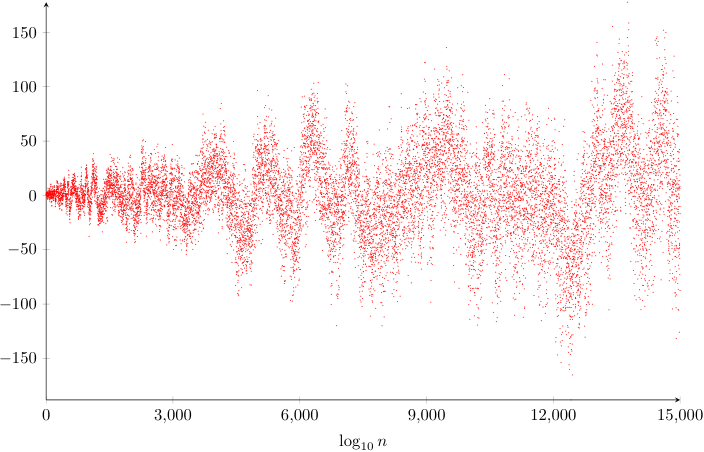
Refer to caption — Figure 13. Deviation of $M(n)$ from $C\cdot(\log 3n)^{2}$ .

References

[Aig13] M. Aigner. Markov’s theorem and 100 years of the uniqueness conjecture. Springer, 2013.
[Bae01] S. I. Baek. Weak local dimension on deranged Cantor sets. Real Anal. Exch., 26(2):553–558, 2001.
[Bae04] S. I. Baek. Spectra of deranged Cantor set by weak local dimensions. J. Math. Kyoto Univ., 44(3):493–500, 2004.
[Bar96] A. Baragar. On the unicity conjecture for Markoff numbers. Canad. Math. Bull., 39(1):3–9, 1996.
[Bow96] B. H. Bowditch. A proof of McShane’s identity via Markoff triples. Bull. London Math. Soc., 28(1):73–78, 1996.
[BU04] A. Baragar and K. Umeda. The asymptotic growth of integer solutions to the Rosenberger equations. Bull. Austral. Math. Fr., 69(3):481–497, 2004.
[But01] J. O. Button. Markoff Numbers, Principal Ideals and Continued Fraction Expansions. J. Number Theory, 87(1):77–95, 2001.
[Cas57] J. W. S. Cassels. An introduction to Diophantine approximation. Number 45 in Cambridge Tracts in Mathematics and Mathematical Physics. Cambridge University Press, 1957.
[CF89] T. W. Cusick and M. E. Flahive. The Markoff and Lagrange spectra. Number 30 in Mathematical Surveys and Monographs. American Mathematical Society, 1989.
[Coh55] H. Cohn. Approach to Markoff’s minimal forms through modular functions. Annals of Mathematics, 61(1):1–12, 1955.
[DL85] J. M. Drezet and J. Le Potier. Fibrés stables et fibrés exceptionnels sur $\mathbb{P}_{2}$ . Ann. scient. Éc. Norm. Sup. $4^{e}$ série, 18:193–244, 1985.
[Fal97] K. Falconer. Techniques in fractal geometry. John Wiley & Sons, 1997.
[Fro68] G. Frobenius. Über die Markoffschen Zahlen. In Gesammelte Abhandlungen, Band III, pages 598–627. Springer, 1968.
[GKP94] R. Graham, D. Knuth, and O. Patashnik. Concrete mathematics. Addison-Wesley, 2nd edition, 1994.
[Hac13] P. Hacking. Exceptional bundles associated to degenerations of surfaces. Duke Math. J., 162(6):1171–1202, 2013.
[HP08] L. Hille and M. Perling. Exceptional sequences of invertible sheaves on rational surfaces. arXiv:0810.1936, 2008.
[HP10] P. Hacking and Y. Prokhorov. Smoothable del Pezzo surfaces with quotient singularities. Compos. Math., 146(1):169–192, 2010.
[JS95] H. Jürgensen and L. Staiger. Local Hausdorff dimension. Acta Informatica, 32:491–507, 1995.
[Kos14] T. Koshy. Pell and Pell-Lucas numbers with applications. Springer, 2014.
[KS88] J. Kollár and N. Shepherd-Barron. Threefolds and deformations of surface singularities. Invent. Math., 91(2):299–338, 1988.
[LT07] M. L. Lang and S. P. Tan. A simple proof of the Markoff conjecture for prime powers. Geom. Dedicata, 129:15–22, 2007.
[Per54] O. Perron. Die Lehre von den Kettenbrüchen, Bd. I. Teubner, 3rd edition, 1954.
[Per18] M. Perling. Combinatorial aspects of exceptional sequences on (rational) surfaces. Math. Z., 288(1–2):243–286, 2018.
[Reu19] C. Reutenauer. From Christoffel words to Markoff numbers. Oxford University Press, 2019.
[Rud89] A. N. Rudakov. Markov numbers and exceptional bundles on $\mathbb{P}^{2}$ . Math. USSR Izvestiya, 32(1):99–112, 1989.
[Slo] N. J. A Sloane. The Online Encyclopedia of Integer Sequences. Published electronically at http://oeis.org.
[Wah81] J. Wahl. Smoothings of normal surface singularities. Topology, 20(3):219–246, 1981.
[Zag82] D. Zagier. On the number of Markoff numbers below a given bound. Math. Comp., 39(160):709–723, 1982.

(	$e$ ,	$g$ ,	$f$	)
(	$r_{e}$ ,	$r_{g}$ ,	$r_{f}$	)
(	$s_{e}$ ,	$s_{g}$ ,	$s_{f}$	)

(	$e$ ,	$F$ ,	$g$	)
(	$r_{e}$ ,	$r_{F}$ ,	$r_{g}$	)
(	$s_{e}$ ,	$s_{F}$ ,	$s_{g}$	)

(	$g$ ,	$E$ ,	$f$	)
(	$r_{g}$ ,	$r_{E}$ ,	$r_{f}$	)
(	$s_{g}$ ,	$s_{E}$ ,	$s_{f}$	)

(	194,	2897,	5	)
(	75,	1120,	2	)
(	29,	433,	1	)

(	433,	37666,	29	)
(	179,	15571,	12	)
(	74,	6437,	5	)

(	$e$ ,	$g$ ,	$f$	)
(	$w_{e}$ ,	$w_{g}$ ,	$w_{f}$	)
(	$v_{e}$ ,	$v_{g}$ ,	$v_{f}$	)

		$\displaystyle 3,(1,5)_{n-2}$	$\displaystyle\text{ if $n$ is even},$
		$\displaystyle(1,5)_{n-1}$	$\displaystyle\text{ if $n$ is odd}.$

		$\displaystyle 6,(4,8)_{n-2},3$	$\displaystyle\text{ if $n$ is even},$
		$\displaystyle(4,8)_{n-1},3$	$\displaystyle\text{ if $n$ is odd}.$

(	1,	13,	5	)
(	0,	5,	2	)
(	1,	2,	1	)

(	1,	34,	13	)
(	0,	13,	5	)
(	1,	5,	2	)

(	1,	89,	34	)
(	0,	34,	13	)
(	1,	13,	5	)

(	34,	1325,	13	)
(	13,	507,	5	)
(	5,	194,	2	)