ADMM based Fourier phase retrieval with untrained generative prior

The untrained generative network incorporates implicit priors about the signals they generate, and these prior assumptions are built into the network structure. Thus we expand the components of the network in detail and analyze the prior information that may be carried by its structure.

Under the untrained generative prior, $\mathbb{S}$ in (1) represents the range of a network which is denoted by $\mathbf{G}(\mathbf{w};\mathbf{z})$. The input $\mathbf{z}\in\mathbb{R}^{d}(d\ll n)$ of network represents the low-dimensional latent code, its elements are fixed and generated from uniform random distribution; $\mathbf{w}$ represents the weights that need to be learned but not pre-trained. This paper draws on the network structure in [31], which exchanges the order of upsampling with a composition of activation function and channel normalization compared to deep decoder [20].

For a $J$-layer network, we denote the input of $j+1$-th layer as $Z_{j}\in\mathbb{R}^{c_{j}\times d_{j}}$ ($j=0,1,\cdots,J-1$) and $Z_{J}\in\mathbb{R}^{c_{J}\times d_{J}}$ represents the output of $J$-th layer, in addition, $\mathbf{z}=vec(Z_{0})$ and $d=c_{0}\times d_{0}$. The network consists of $1\times 1$ convolutions’ weights $W_{j}\in\mathbb{R}^{c_{j+1}\times c_{j}}$, ReLU activation function $relu(\cdot)$, channel normalization operator $cn(\cdot)$ and bi-linear upsampling operators $U_{j}$. The operators from the last layer to the output includes the $1\times 1$ convolutions’ weight $W_{J}\in\mathbb{R}^{c_{out}\times c_{J}}$ and sigmoid activation function $sig(\cdot)$, where $c_{out}=1$ for a grayscale image and $c_{out}=3$ for an RGB image. Thus, the network at layer $j+1$ can be expressed as

The output of network is $G(\mathbf{w};\mathbf{z})=sig\left(W_{J}Z_{J}\right)$, where $\mathbf{w}=\{W_{0},W_{1},\cdots,W_{J}\}$ are weights to learn. It’s apparent that the manually adjustable parameters of the network are network depth and number of weight channels in each layer. We can use $\{c_{0},c_{1},\cdots,c_{J}\}$ to represent the designed structure for a $J$-layer network. Additionally, simplifying (2) gives

where $\mathcal{Z}_{j}\mbox{ }(j=0,1,\cdots,J)$ denote the linear operators in the network because the $1\times 1$ convolution which is the operation between $\mathcal{Z}_{j}$ and $\mathbf{w}$ can be viewed as a linear combination of their channels, $\sigma_{j}=U_{j}\circ cn\circ relu\mbox{ }(j=0,1,\cdots,J-1)$ denote the composite operators of ReLU activation function, channel normalization operator and bi-linear upsampling, $\sigma_{J}=sig$ denotes the sigmoid activation function. These operators are fixed, thus the network can be regarded as a function of $\mathbf{w}$.

Our goal is to find optimal weights $\mathbf{w}^{\ast}$ to represent the optimal solution $\mathbf{x}^{\ast}$, which is equivalent to substituting the surjective mapping [31] $G:\mathbf{w}\to\mathbf{x}$ and minimizing the loss function (4) over $\mathbf{w}$,

where $\mathbb{W}$ denotes the set of weights. Inspired by [34], we can obtain the existence of the solution of model (4).

Note that the conclusion in [34] assumes all free parameters in $F(\mathbf{w})$ are trained before minimization of (4), it is also satisfied here since the untrained generative network (2) does not require to be pre-trained and all operators are fixed. Furthermore, theorem 1 requires that the set of weights $\mathbb{W}$ is a closed set. We can use strategies such as weight decay and so on in the learning process of network to ensure that the condition is satisfied.

For the convenience of algorithm implementation, we rewrite the model (4) as the following optimization model by using the intermediate variable $\mathbf{x}$.

In this section, we will design an algorithm to solve (5), which combines the ADMM with untrained generative network, thus it’s called Net-ADM method in this paper. Firstly, in order to execute Fourier transform by FFT algorithm, we introduce an auxiliary variable $\mathbf{u}\in\mathbb{R}^{m}\mbox{ }(m>n)$ whose last $m-n$ elements are zeros $\mathbf{u}_{[n+1:m]}=0$ such that $\mathcal{F}$ represents FFT operator. Secondly, in order to make the objective function $\psi(\cdot)$ Lipschitz differential, inspired by Chang [35], we add a penalty $\varepsilon\mathbf{1}$ on both sides of $\mathbf{b}=|\mathcal{F}\mathbf{u}|$, then use radical smoothing, the loss function $\psi(\mathbf{x})$ can be rewritten as follows:

where $\varepsilon>0$ represents penalization parameter, $\mathbf{1}\in\mathbb{R}^{m}$ represents a vector whose elements are all ones. The gradient of $f(\mathbf{u})$ is shown in (7), its continuity is proved in Lemma 1.

Note that $\mathbf{u}_{[n+1:m]}=0$ is equivalent to $\mathbf{u}-\mathcal{P}\mathcal{P}^{T}\mathbf{u}=0$. The optimization model (5) now turns to

where $\mathcal{P}:\mathbb{R}^{n}\to\mathbb{R}^{m}$ denotes zero padding operator, i.e. it appends $m-n$ zero elements after the last element of the vector. And $\mathcal{P}^{T}:\mathbb{R}^{m}\to\mathbb{R}^{n}$ means to obtain the first $n$ elements of the vector. The solution of (5) is $\mathbf{x}^{\ast}=\mathcal{P}^{T}\mathbf{u}^{\ast}$, if $\mathbf{u}^{\ast}$ is a solution of (11).

We divide (11) into two sub-problems and solve them alternately. Firstly, taking the objective function (11a) and the first constraint (11b) into consideration, we replace the variable $\mathcal{P}^{T}\mathbf{u}$ with $\mathbf{x}\in\mathbb{R}^{n}$ in (11b), then ADMM can be adopted to solve the following sub-problem alternately.

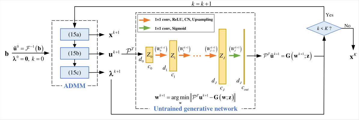
Secondly, we transform the second constraint (11c) into the second sub-problem. The untrained generative network approximates the intermediate variable $\mathcal{P}^{T}\hat{\mathbf{u}}$ of ADMM, aiming to project it into the range of $\mathbf{G}(\mathbf{w};\mathbf{z})$, which captures some characteristics of images.

We can get weights $\hat{\mathbf{w}}$ to represent the substitute variable $\mathcal{P}^{T}\mathbf{\tilde{u}}=\mathbf{G}(\hat{\mathbf{w}};\mathbf{z})$ of $\mathcal{P}^{T}\hat{\mathbf{u}}$, then $\mathcal{P}^{T}\mathbf{\tilde{u}}$ is applied to next iteration of ADMM. The specific execution process can be found in the illustration of the algorithm, as shown in Fig.1.

According to augmented Lagrange multiplier method, we can transform (12) into an unconstrained optimization problem:

where $\bm{\lambda}\in\mathbb{R}^{m}$ is the Lagrangian multiplier associated with the equality constraint, $\rho>0$ is the coefficient of the quadratic penalty term. Therefore, we can minimize $L_{\rho}(\mathbf{x},\mathbf{u},\bm{\lambda})$ with respect to $\mathbf{u}$ and $\mathbf{x}$ in an alternating way, which is the basic idea of ADMM. After obtaining the intermediate variable $\hat{\mathbf{u}}$ of the ADMM, the untrained generative network is used to optimize (13) over $\mathbf{w}$. The variable $\mathcal{P}^{T}\mathbf{\tilde{u}}=\mathbf{G}(\hat{\mathbf{w}};\mathbf{z})$ represented by the network is applied to next iteration. Specifically, given some initial vectors $\mathbf{\tilde{u}}^{0},\bm{\lambda}^{0}$, we can update the variables in the following iterative format:

The optimality conditions of (15a) and (15b) are

According to optimality conditions (16a), (15a) can be expressed explicitly as (17a).

However, it is difficult to obtain an explicit solution of the implicit equation (16b). Thus we first use $\tilde{\mathbf{u}}^{k}$ to approximate $\mathbf{u}^{k+1}$, then the gradient descent algorithm is adopted to solve the expression of $\mathbf{u}^{k+1}$. According to (17a), we have

where we set $\mathbf{\tilde{u}}^{k}_{[n+1:m]}=\bm{\lambda}^{k}_{[n+1:m]}/\rho$. Then it’s straightforward to show that $\nabla_{\mathbf{u}}L_{\rho}(\mathbf{x}^{k+1},\mathbf{\tilde{u}}^{k},\bm{\lambda}^{k})=\nabla f(\mathbf{\tilde{u}}^{k})-\bm{\lambda}^{k}-\rho\left(\mathcal{P}\mathbf{x}^{k+1}-\mathbf{\tilde{u}}^{k}\right)=\nabla f(\mathbf{\tilde{u}}^{k})$. By gradient descent, it follows that

Substituting (7) and (18) into the expression of $\mathbf{u}^{k+1}$ gives rise to (17b).

Note that there is already algorithm [36] for solving FPR problem using ADMM, we can also only solve sub-problem (12) with ADMM, but adding an untrained generative network can reduce the requirement for sampling rates. Since the untrained generative network has a self-regularizing property [37], i.e. the network recovers a natural image at low sampling rate when trained with gradient descent until convergence. Therefore, We use the untrained generative network to project the estimated signal $\mathcal{P}^{T}\hat{\mathbf{u}}$ of ADMM to the range $\mathbb{S}$, getting the Net-ADM algorithm.

Since the model (5) is non-convex, it is hard to ensure the algorithm converges to the optimal solution $\mathbf{x}^{\ast}=\mathcal{P}^{T}\mathbf{u}^{\ast}$. Although the ADMM algorithm has a theoretical guarantee [38] of convergence to a stable point under some conditions, the stable point may be far from the optimal solution due to the non-convexity of the model. We will show that the two projections included in the Net-ADM algorithm have good properties, one of which makes the objective function $f(\mathbf{u})$ descent and the other gets the estimation closer to the optimal solution.

Since the generative space $\mathbb{S}=\{\mathbf{G}(\mathbf{w};\mathbf{z}):\mathbf{w}\in\mathbb{W}\}$ captures some characteristics of the images, we assume that the optimal solution is in the generative space $\mathbf{x}^{\ast}\in\mathbb{S}$. Here we study the mutual projections of the sequences $(\mathcal{P}^{T}\mathbf{u}^{k},\mathcal{P}^{T}\mathbf{\tilde{u}}^{k})$. Let $g(\mathbf{\tilde{u}}^{k})=\mathbf{\tilde{u}}^{k}-\nabla f(\mathbf{\tilde{u}}^{k})$, then

If we set $\mathbb{G}=\left\{\mathcal{P}^{T}g(\mathbf{\tilde{u}}):\mathbf{\tilde{u}}\in\mathbb{R}^{m}\right\}$, then the points in $\mathbb{S}$ can be projected into $\mathbb{G}$ through setting $\mathbf{\tilde{u}}^{k}_{[n+1:m]}=\bm{\lambda}^{k}_{[n+1:m]}/\rho$ and the function $\mathcal{P}^{T}g:\mathbb{R}^{m}\to\mathbb{R}^{n}$. And (15d) and (15e) are projections from $\mathbb{G}$ to $\mathbb{S}$. Thus, given $\mathcal{P}^{T}\mathbf{\tilde{u}}^{0}$ (note that although $\mathcal{P}^{T}\mathbf{\tilde{u}}^{0}$ may not be in $\mathbb{S}$, $\mathcal{P}^{T}\mathbf{u}^{1}$ is in $\mathbb{G}$), the mappings between sequences $\mathcal{P}^{T}\mathbf{u}^{k}$ and $\mathcal{P}^{T}\mathbf{\tilde{u}}^{k}\mbox{ }(k=1,2,\cdots,K)$ in Net-ADM can be viewed as the alternate projections between $\mathbb{S}$ and $\mathbb{G}$, as shown in Fig.2. Note that $\mathbf{x}^{\ast}\in\mathbb{S}\cap\mathbb{G}$ since $\mathbf{x}^{\ast}=\mathcal{P}^{T}\mathbf{u}^{\ast}=\mathcal{P}^{T}g(\mathbf{u}^{\ast})$ and $\mathbf{x}^{\ast}\in\mathbb{S}$.

Here we can get some good properties about the projections.

To compare the reconstruction performance of ADMM, Net-GD, Net-PGD and Net-ADM algorithms at different sampling rates, we implement FPR at ten sampling rates (ranging from $1.1:0.1:2.0$) on the MNIST and CelebA respectively. Each algorithm was run ten times for each image at each sampling rate, and the average PSNR and SSIM of the reconstructed images were calculated as the mean of these ten runs.

Fig.3 shows the average PSNR and SSIM of the images reconstructed by the four algorithms at different sampling rates. The results show that the average PSNR and SSIM of Net-ADM’s reconstructed results are higher than those of the other three algorithms in most instances, especially when $r<1.7$. Although the average PSNR and SSIM of ADMM’s reconstructed results might be higher than those of Net-ADM when $1.7<r\leq 2.0$, they decreases rapidly when the sampling rates are lower than 1.7 (for MNIST) or 1.8 (for CelebA), which shows that ADMM has higher requirements for sampling rates. When $r>1.7$, the reason why Net-ADM is sometimes slightly worse than ADMM may be that the number of parameters of the untrained generative network is not enough to accurately fit the high-quality estimation $\mathcal{P}^{T}\mathbf{u}$ generated by ADMM. After all, we have to make a trade-off between fitting error and stability. Comparatively, Net-GD, Net-PGD and Net-ADM are more stable with the decrease of sampling rates, which is in fact more challenging for FPR especially in applications where the resolution of the measurement device is low. Among them, the average PSNR and SSIM of images reconstructed by Net-ADM are higher than those of Net-GD and Net-PGD.

Fig.4 shows the best reconstructed images (on MNIST and CelebA) in ten runs at sampling rates $r=1.1:0.1:1.6$ and $r=1.6:0.1:2.0$ respectively. Fig.5 shows the best reconstructed images on Cameraman from ten runs of the four algorithms at sampling rate $r=1.7$ and $r=1.6$ respectively. From the experiment results, the reconstruction quality using Net-ADM is superior to others. Although ADMM seems to work better when the sampling rate is high, it’s unstable such as the reconstruction quality of CelebA5 at $r=2.0$ is poor. Additionally, the reconstructed results of Net-GD and Net-PGD are not as good as Net-ADM. Thus, the reconstructed results of Net-ADM at different sampling rates are superior and stable by contrast.

In this section, we compare the robustness of Net-ADM with other algorithms in resisting measurement noise. The noisy measurement model is:

where $\eta$ is Gaussian noise, i.e. $\eta\sim N(0,\sigma^{2})$.

Under fixed sampling rates, we compare the PSNR and SSIM of the images reconstructed by four algorithms when the measurements are affected by noise of different levels. The noise level is measured by Signal Noise Ratio (SNR), the formula for calculating SNR is as follows:

where ${\rm Var}(\left|\mathcal{F}\mathbf{x}\right|)$ calculates the variance of the noiseless magnitude measurement $\left|\mathcal{F}\mathbf{x}\right|$. At each SNR we will randomly generate 10 different Gaussian noise.

We choose CelebA3 image, add noise of different levels (SNR ranging from 20:10:70dB) to the measurements under four fixed sampling rates, and compare the PSNR and SSIM of the reconstructed results of the four algorithms. The average PSNR and SSIM of ten runs are shown in Table 1. In addition, we choose Cameraman image, add noise of SNR=60dB and SNR=30dB to the magnitude measurements respectively at sampling rate $r=2.0$, the best results in ten runs are shown in Fig.6.

It is observed from the experiment results that the PSNR and SSIM of Net-ADM’s reconstructed results are basically higher than those of other three algorithms under different SNR and sampling rates. The robustness of Net-ADM is significantly improved compared to ADMM, even though the PSNR and SSIM of their reconstructed results decrease as the sampling rates and SNR decrease. The PSNR and SSIM of the images reconstructed by Net-GD and Net-PGD remains stable with the change of sampling rates and SNR, but Net-ADM’s constructed results maintain the highest PSNR and SSIM in most situations, indicating that Net-ADM has superior robustness.

Now we consider the effect of parameters in Net-ADM. Because the ADMM is not highly sensitive to the choice of the relaxation parameter $\rho$ [36], we don’t discuss too much about $\rho$ here. Since the design of the architecture will affect the representation range of the network, we explore the important parameters that affect the network architecture. Due to the particular choice of the input $\mathbf{z}$ is not very important [20] but it is necessary to ensure that the lines are not coherent, we won’t explore exhaustively here. Upsampling is a vital part of network, it has been discussed in [20] that linear upsampling is better able to represent smoothly varying portions of the signal compared with no upsampling, nearest neighbor upsampling, convex and non-linear upsampling. Regarding other tunable parameters of the untrained generative network, we compare the reconstructed results of Net-ADM at different network depths, number of weight channels and activation functions. Net-ADM is run ten times at each sampling rate in all experiments.

In order to evaluate the impact of network depth, we fix the channel number in each layer of the network to 64 and the activation function to ReLU, and compare the reconstructed results of Net-ADM on Cameraman with different network depths. The PSNR of the reconstructed results are shown in Fig.7 (a). Although the PSNR of reconstructed image under network depth $J=3$ is low slightly than $J=2$ sometimes, it remains stable interval in all situations. Taking the average quality and stability of the reconstruction into account, we choose the network depth to be 3.

Then in the case where the network depth is 3 and the activation function is ReLU, we compare the impact of the number of weight channels, as shown in Fig.7 (b). It can be seen that the PSNR of reconstructed image under different channel numbers is slightly different, but we choose the relatively optimal scheme, which is {128, 64, 64, 32}.

In the case where the number of network channels is designed by {128, 64, 64, 32}, we reconstruct image under different activation functions, the average values in the PSNR interval out of ten runs are shown in Fig.8. Except for the Sigmoid activation function, the effects of these activation functions are not significantly different when sampling rates are high, but the opposite when sampling rates are low. Thus, we choose the ReLU activation function which is relatively stable.

References

- [1] J. J. Miao, T. Ishikawa, Q. Shen, T. N. Earnest, Extending x-ray crystallography to allow the imaging of noncrystalline materials, cells, and single protein complexes, Annu. Rev. Phys. Chem. 59 (1) (2008) 387–410, https://dx.doi.org/10.1146/annurev.physchem.59.032607.093642.
- [2] S. Pinilla, H. García, L. Díaz, J. Poveda, H. Arguello, Coded aperture design for solving the phase retrieval problem in x-ray crystallography, J. Comput. Appl. Math. 338 (2018) 111–128, https://dx.doi.org/10.1016/j.cam.2018.02.002.
- [3] P. Chen, A. Fannjiang, Coded aperture ptychography: Uniqueness and reconstruction, Inverse Probl. 34 (2) (2018) 025003(1–26), https://dx.doi.org/10.1088/1361-6420/aa9ef4.
- [4] D. R. Luke, Relaxed averaged alternating reflections for diffraction imaging, Inverse Probl. 21 (1) (2005) 37–50, https://dx.doi.org/10.1088/0266-5611/21/1/004.
- [5] J. C. Dainty, J. R. Fienup, Phase retrieval and image reconstruction for astronomy, in: Image Recovery: Theory and Application, Vol. 231, 1987, p. 275.
- [6] A. Fannjiang, T. Strohmer, The numerics of phase retrieval, Acta Numer. 29 (2020) 125–228, https://dx.doi.org/10.1017/S0962492920000069.
- [7] R. Balan, P. Casazza, E. Dan, On signal reconstruction without phase, Appl. Comput. Harmon. Anal. 20 (3) (2006) 345–356, https://dx.doi.org/10.1016/j.acha.2005.07.001.
- [8] E. J. Candès, T. Strohmer, V. Voroninski, Phaselift: Exact and stable signal recovery from magnitude measurements via convex programming, Commun. Pur Appl. Math. 66 (8) (2013) 1241–1274, https://dx.doi.org/10.1002/cpa.21432.
- [9] T. Goldstein, C. Studer, Phasemax: Convex phase retrieval via basis pursuit, IEEE Trans. Inf. Theory 64 (4) (2018) 2675–2689, https://dx.doi.org/10.1109/TIT.2018.2800768.
- [10] L. H. Yeh, J. Dong, J. Zhong, L. Tian, M. Chen, G. Tang, M. Soltanolkotabi, L. Waller, Experimental robustness of fourier ptychography phase retrieval algorithms, Opt. Express 23 (26) (2015) 33214–33240, https://dx.doi.org/10.1364/OE.23.033214.
- [11] G. Wang, G. B. Giannakis, Y. C. Eldar, Solving systems of random quadratic equations via truncated amplitude flow, IEEE Trans. Inf. Theory 64 (2) (2018) 773–794, https://dx.doi.org/10.1109/TIT.2017.2756858.
- [12] C.-C. Chen, J. J. Miao, C. W. Wang, T.-K. Lee, Application of optimization technique to noncrystalline x-ray diffraction microscopy: Guided hybrid input-output method, Phys. Rev. B 76 (6) (2007) 064113(1–5), https://dx.doi.org/10.1103/PhysRevB.76.064113.
- [13] P. Sarangi, H. Qiao, P. Pal, On the role of sampling and sparsity in phase retrieval for optical coherence tomography, in: IEEE International Workshop on Computational Advances in Multi-Sensor Adaptive Processing (CAMSAP), 2017, pp. 1–5.
- [14] P. Hand, O. Leong, V. Voroninski, Phase retrieval under a generative prior, in: Advances in Neural Information Processing Systems (NeurIPS), Vol. 31, 2018.
- [15] R. Hyder, V. Shah, C. Hegde, M. S. Asif, Alternating phase projected gradient descent with generative priors for solving compressive phase retrieval, in: IEEE International Conference on Acoustics, Speech and Signal Processing (ICASSP), 2019, pp. 7705–7709, https://dx.doi.org/10.1109/ICASSP.2019.8682811.
- [16] F. Shamshad, A. Ahmed, Robust compressive phase retrieval via deep generative priors, IEEE Sens. J. 21 (2) (2021) 2286–2298, https://dx.doi.org/10.1109/JSEN.2020.3018751.
- [17] G. Jagatap, C. Hegde, Phase retrieval using untrained neural network priors, in: NeurIPS Workshop on Solving Inverse Problems with Deep Networks, 2019.
- [18] R. Hyder, C. Hegde, M. S. Asif, Fourier phase retrieval with side information using generative prior, in: Asilomar Conference on Signals, Systems, and Computers, 2019, pp. 759–763.
- [19] D. Ulyanov, A. Vedaldi, V. Lempitsky, Deep image prior, Int. J. Comput. Vision 128 (7) (2020) 1867–1888, https://dx.doi.org/10.1007/s11263-020-01303-4.
- [20] R. Heckel, P. Hand, Deep decoder: Concise image representations from untrained non-convolutional networks, in: International Conference on Learning Representations (ICLR), 2019.
- [21] R. W. Gerchberg, A. S. W. O., A practical algorithm for the determination of phase from image and diffraction plane pictures, Optik 35 (2) (1972) 237–246.
- [22] J. R. Fienup, Phase retrieval algorithms: a comparison., Appl. Opt. 21 (15) (1982) 2758–2769, https://dx.doi.org/10.1364/AO.21.002758.
- [23] E. J. Candès, X. Li, M. Soltanolkotabi, Phase retrieval via wirtinger flow: Theory and algorithms, IEEE Trans. Inf. Theory 61 (4) (2015) 1985–2007, https://dx.doi.org/10.1109/TIT.2015.2399924.
- [24] Y. Chen, E. J. Candès, Solving random quadratic systems of equations is nearly as easy as solving linear systems, Commun. Pure Appl. Math. 70 (5) (2015) 822–883, https://dx.doi.org/10.1002/cpa.21638.
- [25] Z. Yuan, H. Wang, Q. Wang, Phase retrieval via sparse wirtinger flow, J. Comput. Appl. Math. 355 (2019) 162–173, https://dx.doi.org/10.1016/j.cam.2019.01.009.
- [26] C. Ma, X. Liu, Z. Wen, Globally convergent levenberg-marquardt method for phase retrieval, IEEE Trans. Inf. Theory 65 (4) (2019) 2343–2359, https://dx.doi.org/10.1109/TIT.2018.2881187.
- [27] C. A. Metzler, P. Schniter, A. Veeraraghavan, R. G. Baraniuk, prdeep: Robust phase retrieval with a flexible deep network, in: In International Conference on Machine Learning (PMLR), 2018, pp. 3501–3510.
- [28] I. Ç, O. FS, K. A, Deep iterative reconstruction for phase retrieval, Appl. Opt. 58 (20) (2019) 5422–5431, https://dx.doi.org/10.1364/AO.58.005422.
- [29] A. T. Sinha, J. Lee, S. Li, G. Barbastathis, Lensless computational imaging through deep learning, Optica 4 (9) (2017) 1117–1125, https://dx.doi.org/10.1364/OPTICA.4.001117.
- [30] M. J. Cherukara, Y. S. G. Nashed, R. J. Harder, Real-time coherent diffraction inversion using deep generative networks, Sci. Rep. 8 (1) (2018) 1–8, https://dx.doi.org/10.1038/s41598-018-34525-1.
- [31] G. Jagatap, C. Hegde, Algorithmic guarantees for inverse imaging with untrained network priors, in: Advances in neural information processing systems (NeurIPS), Vol. 32, 2019.
- [32] A. S. Bandeira, J. Cahill, D. G. Mixon, A. A. Nelson, Saving phase: Injectivity and stability for phase retrieval, Appl. Comput. Harmon. Anal. 37 (1) (2014) 106–125, https://dx.doi.org/10.1016/j.acha.2013.10.002.
- [33] D. Potts, M. Tasche, Numerical stability of nonequispaced fast fourier transforms, J. Comput. Appl. Math. 222 (2) (2008) 655–674, https://dx.doi.org/10.1016/j.cam.2007.12.025.
- [34] H. Li, J. Schwab, S. Antholzer, M. Haltmeier, Nett: solving inverse problems with deep neural networks, Inverse Probl. 36 (6) (2020) 1–23, https://dx.doi.org/10.1088/1361-6420/ab6d57.
- [35] H. Chang, P. Enfedaque, S. Marchesini, Blind ptychographic phase retrieval via convergent alternating direction method of multipliers, SIAM J. Imag. Sci. 12 (1) (2019) 153–185, https://dx.doi.org/10.1137/18M1188446.
- [36] Z. Wen, C. Yang, X. Liu, S. Marchesini, Alternating direction methods for classical and ptychographic phase retrieval, Inverse Probl. 28 (11) (2012) 115010(1–18), https://dx.doi.org/10.1088/0266-5611/28/11/115010.
- [37] R. Heckel, M. Soltanolkotabi, Compressive sensing with un-trained neural networks: Gradient descent finds the smoothest approximation, in: International Conference on Machine Learning (PMLR), 2020, pp. 4149–4158.
- [38] Y. Lou, M. Yan, Fast l1–l2 minimization via a proximal operator, J. Sci. Comput. 74 (2) (2018) 767–785, https://dx.doi.org/10.1007/s10915-017-0463-2.