Fast Beam Alignment via Pure Exploration in Multi-armed Bandits

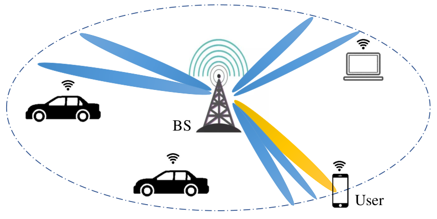
As shown in Fig. 1, we consider a massive mmWave MISO system, where a base station (BS) equipped with $N$ transmit antennas serves a single-antenna user. According to [23], each transmitting beam is selected from a predefined analog beamforming codebook $\mathcal{C}$ of size $K$, which can be defined as

with $\mathbf{a}(\cdot)$ denoting the array response vector. For a typical uniform linear array, it holds that $\mathbf{a}(x)=\frac{1}{\sqrt{N}}\big[1,e^{j\frac{2\pi}{\lambda}dx},e^{j\frac{2\pi}{\lambda}2dx},\ldots,e^{j\frac{2\pi}{\lambda}(N-1)dx}\big]^{\mathrm{H}}\in\mathbb{C}^{N\times 1},$ where $\lambda$ is the wavelength and $d$ is the antenna spacing. Note that if $K\leq N$, the beams in the codebook $\mathcal{C}$ are linearly independent of one another. Based on channel measurement studies done in [24, 25], the mmWave channel follows a multipath channel model, and the number of propagation paths is small.

We consider a quasi-static channel, where the channel stays unchanged for a period covariance interval which consists of $T$ time slots. As shown in Fig. 2, each covariance interval can be divided into two phases, the BA phase (which consists of $T_{\mathrm{B}}$ time slots) and the data transmission phase (which consists of $T_{\mathrm{D}}=T-T_{\mathrm{B}}$ time slots). With the selected beam $\mathbf{f}$, the effective achievable rate (EAR) of each covariance interval

is widely accepted as a metric to measure the throughput performance, where $p$ and $\sigma^{2}$ represent the transmit power and noise variance respectively. We observe that the throughput performance increases with the decreasing $T_{\mathrm{B}}/T_{\mathrm{D}}$ and increasing $|\mathbf{h}^{\mathrm{H}}\mathbf{f}^{*}|^{2}$. As such, the time allocated for selecting the optimal beam $\mathbf{f}^{*}=\argmax_{\mathbf{f}\in\mathcal{C}}|\mathbf{h}^{\mathrm{H}}\mathbf{f}|^{2}$ should be minimized for higher system throughput, which is the motivation of this work.

In the BA phase, the BS selects one beam from the codebook $\mathcal{C}$ and transmits pilot signals to the user with this beam. Without loss of generality, we set the pilot signal to be $1$. Then the received power can be expressed as

where $n^{*}$ represents the complex conjugate of the complex Gaussian noise $n\sim\mathcal{CN}(0,\sigma^{2})$. Note that the BS can observe the received power from the user through a feedback link, and this assumption is also adopted in other studies such as [20, 21]. We can see that $R(\mathbf{f}_{k})$ is a random variable which is the sum of a Gamma random variable $|n|^{2}\sim\Gamma(1,1/\sigma^{2})$ and a Gaussian random variable $p|\mathbf{h}^{\mathrm{H}}\mathbf{f}_{k}|^{2}+2\sqrt{p}\Re(\mathbf{h}^{\mathrm{H}}\mathbf{f}_{k}n^{*})\sim\mathcal{N}(p|\mathbf{h}^{\mathrm{H}}\mathbf{f}_{k}|^{2},2p|\mathbf{h}^{\mathrm{H}}\mathbf{f}_{k}|^{2}\sigma^{2})$. Fig. 3 shows the average received power associated with different beams over the codebook space when $K=120$, $N=64$, $p=26$ dBm and the power of LoS path is around 3 dB larger than those of the NLoS paths. It can be observed that all the received powers become larger as the increase of the noise variance, and the improved value is the difference between the noise variances. Since the noise variance is much smaller than the transmit power, the variable $R(\mathbf{f}_{k})$ is approximately a Gaussian random variable with mean $\mu_{k}=p|\mathbf{h}^{\mathrm{H}}\mathbf{f}_{k}|^{2}$ and variance $\sigma^{2}_{k}=2p|\mathbf{h}^{\mathrm{H}}\mathbf{f}_{k}|^{2}\sigma^{2}$, i.e.,

The optimal beam is defined as the beam that has the largest value of $r_{k}$, i.e., ${k}^{*}=\argmax_{k}p|\mathbf{h}^{\mathrm{H}}\mathbf{f}_{k}|^{2}$.

Let $J$ be the correlation length of arms, which is related to the number of beams $N$ and the size of the codebook $K$ as follows: $J=2\lceil\frac{K}{N}\rceil-1$. Then the received power using the beam $\mathbf{f}_{k}$ and the nearby beam $\mathbf{f}_{i},|k-i|\leq J/2$ are similar. A new $\frac{1}{J}$-lower resolution beam codebook $\mathcal{C}_{(J)}$ can be constructed by grouping the nearby beams in the codebook $\mathcal{C}$, i.e.,

where the beams $\mathbf{b}_{g}$’s are normalized (to unit $\ell_{2}$ norm) to mimic reality in a phased array. If we choose a beam $\mathbf{b}_{g}$ in the codebook $\mathcal{C}_{(J)}$, the received power can be expressed as

Since the received powers associated with the nearby beams in the codebook $\mathcal{C}$ have means that are close to one another, $R_{g}$ has large mean if $r_{k},k\in\{(g-1)J+1,\ldots,gJ\}$ have large means.

To introduce the idea of bandit to address the BA problem, we consider a bandit model where the beam $\mathbf{f}_{k}$ is regarded as the base arm $k$, and the received power using this beam is regarded as the reward of the base arm $k$. The means of the rewards when arms are pulled have the following property:

As shown in Fig. 3, Property 1.1 holds because the beam codebook is designed such that beams that are nearby have rewards that are close. Property 1.2 is due to the fact that there are only a few main paths in the considered channel model, which has been corroborated by studies in channel measurements [26]. Finally, Property 1.3 holds because the mean of reward associated with base arm $k$ follows a heteroscedastic Gaussian distribution $\mathcal{N}(\mu_{k},2\mu_{k}\sigma^{2})$ (see (4)). Furthermore, in this work, we focus on a challenging case with large noise, which satisfies that

and this condition is assumed to hold in our theoretical analyses. In the simulations, we also numerically check that this condition holds.

Since a large number of base arms have mean rewards that are close to zero (Property 1.3), it is clearly a waste of BA overhead to search for the optimal arm among all the base arms. To overcome this problem, we propose to group the base arms by utilizing Property 1.1 which says that the means of the reward associated with nearby arms are similar. As such, we can formulate the BA problem as a novel MAB problem, called the bandit BA problem.

In a bandit BA problem with $K$ base arms, the base arm $k$ is associated with the beam $\mathbf{f}_{k}$. We let $[K]=\{1,\ldots,K\}$ and $\binom{[K]}{\leq J}_{\mathrm{consec}}$ be the set of all non-empty consecutive tuples of length $\leq J$ whose element belongs to the set $[K]$, e.g., if $J=2$ and $K=6$,

and we consider each tuple as a $(K,J)$-super arm. Moreover, the super arm associated with $\mathbf{b}_{g}\in\mathcal{C}_{(J)}$ is a subset of $\binom{[K]}{\leq J}_{\mathrm{consec}}$, e.g., $\{\{1,2\},\{3,4\},\{5,6\}\}\subset\binom{[6]}{\leq 2}_{\mathrm{consec}}$. At time step $t$, we choose an action (or a $(K,J)$-super arm) $A(t)\in\binom{[K]}{\leq J}_{\mathrm{consec}}$, and observe the reward $R(t)$ which is related to the base arms included in $A(t)$, i.e.,

where $F(\mathbf{f},p,\mathbf{h},n)=p|\mathbf{h}^{\mathrm{H}}\mathbf{f}|^{2}+2\sqrt{p}\Re(\mathbf{h}^{\mathrm{H}}\mathbf{f}n^{*})$, $n$ is a complex Gaussian random variable with mean zero and variance $\sigma^{2}$. We can conclude that for an arbitrary $(K,J)$-super arm $A\in\binom{[K]}{\leq J}_{\mathrm{consec}}$, the empirical mean $R_{A}$ also follows a heteroscedastic Gaussian distribution, i.e., $R_{A}\sim\mathcal{N}(\mu_{A},2\mu_{A}\sigma^{2})$, where $\mu_{A}=p|\mathbf{h}^{\mathrm{H}}\sum_{k\in{A}}\mathbf{f}_{k}|^{2}$.

To identify the optimal base arm, an agent uses an algorithm $\pi$ that decides which super arms to pull, the time $\tau^{\pi}$ to stop pulling, and which base arm $k^{\pi}$ to choose eventually. An algorithm consists of a triple $\pi:=\{(\pi_{t})_{t},\tau^{\pi},\psi^{\pi},J\}$ in which:

• •

  a sampling rule $\pi_{t}$ determining the $(K,J)$-super arm $A(t)\in\binom{[K]}{\leq J}_{\mathrm{consec}}$ to pull at time step $t$ based on the observation history and the arm history $\{A(1),R(1),A(2),R(2),\ldots,A(t-1),R(t-1)\}$;

• •

  a stopping rule leading to a stopping time $\tau^{\pi}$ satisfying $\mathbb{P}(\tau^{\pi}<\infty)=1$;

• •

  a recommendation rule $\psi^{\pi}$ that outputs a base arm $k^{\pi}\in[K]$.

We define the time complexity of $\pi$ as $\tau^{\pi}$. In the fixed-confidence setting, a maximum risk $\delta\in(0,1)$ is fixed. We say an algorithm $\pi$ is $(\delta,J)$-probably approximately correct (PAC) if $\mathbb{P}(k^{\pi}=k^{*})\geq 1-\delta$. The purpose is to design a $(\delta,J)$-PAC algorithm $\pi$ that minimizes the expected stopping time $\mathbb{E}[\tau^{\pi}]$.

Denote by $\nu$ a $K$-armed heteroscedastic Gaussian bandit instance, $\nu=\big\{\mathcal{N}(\mu^{\nu}_{1},2\mu^{\nu}_{1}\sigma^{2}),$ $\ldots,\mathcal{N}(\mu^{\nu}_{K},2\mu^{\nu}_{K}\sigma^{2})\big\}$. Let $\mathcal{V}$ represent the set of $K$-armed heteroscedastic Gaussian bandit instances such that each bandit instance $\nu\in\mathcal{V}$ has a unique optimal arm: for each $\nu\in\mathcal{V}$, there exists an arm $A^{*}(\nu)$ such that $\mu^{\nu}_{A^{*}(\nu)}>\max\{\mu^{\nu}_{k}:k\neq A^{*}(\nu)\}$. Define $\mathcal{W}_{K}=\big\{\mathbf{w}\in\mathbb{R}_{+}^{K}:\sum_{k=1}^{K}\vphantom{\Big[}w_{k}=1\big\}$, $\operatorname{Alt}(\nu):=\left\{\mathrm{u}\in\mathcal{V}:A^{*}(\mathrm{u})\neq A^{*}(\nu)\right\}$, and $T_{k}(t)$ as the times the base arm $k$ is pulled until time step $t$. Moreover, the KL divergence between two heteroscedastic Gaussian distributions, i.e., $\mathcal{N}(\mu_{i},2\mu_{i}\sigma^{2})$ and $\mathcal{N}(\mu_{j},2\mu_{j}\sigma^{2})$, can be calculated as

According to Theorem 1 of [27], we can obtain the general lower bound of this problem as follows.

Note that the original Track-and-Stop (T&S) [27] is the state-of-the-art best arm identification algorithm with fixed confidence for exponential bandits, which can be modified to solve the bandit BA problem with low sample complexity, resulting in a fast BA solution.

Let $\nu$ represent a $K$-armed Gaussian bandit instance, $\nu=\big\{\mathcal{N}\big(\mu^{\nu}_{1},(\sigma^{\nu}_{1})^{2}\big),\mathcal{N}\big(\mu^{\nu}_{2},(\sigma^{\nu}_{2})^{2}\big),\ldots,$ $\mathcal{N}\big(\mu^{\nu}_{K},(\sigma^{\nu}_{K})^{2}\big)\big\}$. Given the fixed $\delta$, the time complexity of T&S, $\mathbb{E}\left[\tau^{\text{T\&S}}\right]$, satisfies

where

and the KL-divergence $D\left(\mathcal{N}\big(\mu^{\nu}_{k},(\sigma^{\nu}_{k})^{2}\big),\mathcal{N}\big(\mu^{\mathrm{u}}_{k},(\sigma^{\mathrm{u}}_{k})^{2}\big)\right)=\ln\big(\frac{\sigma^{\mathrm{u}}_{k}}{\sigma^{\nu}_{k}}\big)+\frac{(\sigma^{\nu}_{k})^{2}+\left(\mu^{\nu}_{k}-\mu^{\mathrm{u}}_{k}\right)^{2}}{2(\sigma^{\mathrm{u}}_{k})^{2}}-\frac{1}{2}$.

Furthermore, when we apply T&S to the $K$-armed heteroscedastic Gaussian bandit instance $\nu\in\mathcal{V}$ under consideration, we have

where

and the gaps are $\Delta_{\nu,k}:=\mu^{\nu}_{A^{*}(\nu)}-\mu^{\nu}_{k},k\neq A^{*}(\nu)$ and $\Delta_{\nu,\min}:=\min_{k\neq A^{*}(\nu)}\mu^{\nu}_{A^{*}(\nu)}-\mu^{\nu}_{k}$.

For our bandit BA problem, we propose the 2PHT&S algorithm inspired by the original T&S algorithm [27] to achieve a smaller time complexity by leveraging the structure of the BA problem. The main idea of the proposed algorithm is to exploit the prior knowledge which have not been considered by existing algorithms, i.e., Property 1 and the fact that neighboring beams can be grouped and the corresponding “grouped” reward can be observed in one time step.

As shown in Fig. 4, 2PHT&S consists of two phases. We describe them in the following.

• •

  In Phase I, we first group $K$ base arms into $G$ arm sets and accordingly construct a set of super arms as

  $$\mathcal{G}=\{\mathcal{S}_{g}=\{(g-1)J+1,\ldots,gJ\}|g\in[G]\}.$$

  (17)

  According to (9), the reward associated with super arm $\mathcal{S}_{g}$ can be written as $R_{g}(t)=F(\sum_{k\in{S_{g}}}\mathbf{f}_{k},p,\mathbf{h},n_{t})$. Second, we search for the optimal super arm, $g^{*}=\argmax_{\vphantom{\underline{g}}g\in[G]}\mathbb{E}[R_{g}(t)]$, with a high probability of at least $1-\delta_{1}$, where $\delta_{1}$ denotes the maximum allowable risk in Phase I.

• •

  In Phase II, we construct a base arm set (including two super arms) and select the optimal base arm from this base arm set. Considering the case shown in Fig. 5, where the optimal base arm lies in the right edge of the super arm $\mathcal{S}_{g}$ and the second optimal base arm lies in the left edge of the super arm $\mathcal{S}_{g+2}$, the mean of the reward of the super arm $\mathcal{S}_{g+1}$ may be higher than that of the super arm $\mathcal{S}_{g}$. This observation results in a higher difficulty of identifying the optimal super arm. Therefore, to improve the selection accuracy, we construct a base arm set, i.e., the combination of the optimal super arm and either one of its (left or right) neighbors that has the larger mean. Next, we select the optimal base arm in this base arm set with a certain fixed confidence probability of at least $1-\delta_{2}$.

Given the fixed maximum risk $\delta$, risks $\delta_{1}$ and $\delta_{2}$ should satisfy the constraint $\delta=\delta_{1}+\delta_{2}$.¹¹ 1 Note that since the two phases are independent, the probability of selecting the optimal base arm can be expressed as $(1-\delta_{1})(1-\delta_{2})=1-\delta_{1}-\delta_{2}+\delta_{1}\delta_{2}$. Then, the error probability is $\delta_{1}+\delta_{2}-\delta_{1}\delta_{2}$, which is less than $\delta_{1}+\delta_{2}$ since the two phases are independent. For simplicity, for the given fixed confidence $\delta$, we set $\delta_{1}+\delta_{2}=\delta$. The proposed 2PHT&S is detailed in Algorithm 1, where $\hat{\bm{\mu}}^{\mathrm{s}}=[\hat{\mu}^{\mathrm{s}}_{1},\ldots,\hat{\mu}^{\mathrm{s}}_{G}]$ and $\hat{\bm{\mu}}^{\mathrm{b}}=[\hat{\mu}^{\mathrm{b}}_{\mathcal{S}_{f}(1)},\ldots,\hat{\mu}^{\mathrm{b}}_{\mathcal{S}_{f}(2J)}]$ represent the empirical means of super arms and base arms included in $\mathcal{S}_{f}$, respectively. In both of Phase I and Phase II of 2PHT&S, an improved T&S algorithm exploiting the heteroscedastic property, which is referred to as Heteroscedastic Track-and-Stop (HT&S), is leveraged to search for the optimal super arm and the optimal base arm, respectively.

We now introduce the HT&S algorithm. Define a set of $I\in\mathbb{N}$ super arms $\mathcal{I}=\{\mathcal{S}_{1},\ldots,\mathcal{S}_{I}\}$ where the reward $R_{i}(t)$ of super arm $\mathcal{S}_{i}$ is related to the beams $k\in\mathcal{S}_{i}$ as follows: $R_{i}(t)=F(\sum_{k\in{S_{i}}}\mathbf{f}_{k},p,\mathbf{h},n_{t})$. Given $\mathcal{I}$ and the fixed $\delta$, HT&S outputs all the empirical means, $\hat{\bm{\mu}}^{\nu}=[\hat{\mu}^{\nu}_{1},\ldots,\hat{\mu}^{\nu}_{I}]$, and the required number of time steps $\tau$. Let $A(t)$ represent the index of the super arm pulled in time step $t$, i.e., in time step $t$ the super arm $\mathcal{S}_{A(t)}$ is selected by the sampling rule. We observe the following reward associated with the super arm $\mathcal{S}_{A(t)}$ is

Accordingly, we update the number of times each arm is selected up to time step $t$ and their empirical mean as

The search is terminated when the stopping rule (delineated in (21) below) is satisfied. Define the heteroscedastic Gaussian bandit instance at time step $t$ as $\hat{\nu}_{t}=\big\{\mathcal{N}\big(\hat{\mu}^{\nu}_{1}(t),2\hat{\mu}^{\nu}_{1}(t)\sigma^{2}\big),\ldots,\mathcal{N}\big(\hat{\mu}^{\nu}_{I}(t),2\hat{\mu}^{\nu}_{I}(t)\sigma^{2}\big)\big\}$. The stopping rule and sampling rule, which exploit the heteroscedastic property, form the core of HT&S:

1) Stopping rule: We choose the threshold as $\beta(t,{\delta},\alpha)=\ln(\alpha t/{\delta})$, and the stopping rule as

where $Z(t)$ is defined in (22) at the top of the next page, and

Please refer to (64)–(67) in Appendix C for more details of the derivation of $(a)$ in (22).

2) Sampling rule: The sampling rule can be summarized by $Q(t)$ defined in (25) on the top of the next page,

where $\hat{\mathbf{w}}^{*}(t)\in\mathcal{W}_{I}$ is the set of parameters to be updated at time step $t$. Define

and $f_{X,i,t}(y)\triangleq f^{-1}_{Y,i,t}(x_{i})$. The value of $\hat{w}^{*}_{i}(t)$ is set to be

where $y^{*}(t)$ is the unique solution of the equation $\sum_{i\neq A^{*}(\bm{\mu})}{yf^{\prime}_{X,i,t}(y)}-f_{X,i,t}(y)=1$. Note that the choice of $\hat{\mathbf{w}}^{*}(t)$ is determined according to the optimization problem in (12); see the technical details in Appendix C.

It is worth noting that the stopping rule and sampling rule of HT&S are different from those of original T&S, and both of them are derived from the lower bound given in Theorem 1 based on the heteroscedastic property.

References

• [1] Y. Wei, Z. Zhong, V. Y. F. Tan, and C. Wang, “Fast beam alignment via pure exploration in multi-armed bandits,” in IEEE International Symposium on Information Theory (ISIT), 2022, pp. 1886–1891.
• [2] P. Zhou, X. Fang, Y. Fang, Y. Long, R. He, and X. Han, “Enhanced random access and beam training for millimeter wave wireless local networks with high user density,” IEEE Trans. Wireless Commun., vol. 16, no. 12, pp. 7760–7773, 2017.
• [3] M. Giordani, M. Polese, A. Roy, D. Castor, and M. Zorzi, “A tutorial on beam management for 3GPP NR at mmWave frequencies,” IEEE Commun. Surveys Tuts., vol. 21, no. 1, pp. 173–196, 2019.
• [4] S. Noh, M. D. Zoltowski, and D. J. Love, “Multi-resolution codebook and adaptive beamforming sequence design for millimeter wave beam alignment,” IEEE Trans. Wireless Commun., vol. 16, no. 9, pp. 5689–5701, 2017.
• [5] J. Zhang, Y. Huang, Q. Shi, J. Wang, and L. Yang, “Codebook design for beam alignment in millimeter wave communication systems,” IEEE Trans. Commun., vol. 65, no. 11, pp. 4980–4995, 2017.
• [6] M. Xiao, S. Mumtaz, Y. Huang, L. Dai, Y. Li, M. Matthaiou, G. K. Karagiannidis, E. Bjornson, K. Yang, C.-L. I, and A. Ghosh, “Millimeter wave communications for future mobile networks,” IEEE J. Sel. Areas Commun., vol. 35, no. 9, pp. 1909–1935, 2017.
• [7] M. Gao, B. Ai, Y. Niu, Z. Zhong, Y. Liu, G. Ma, Z. Zhang, and D. Li, “Dynamic mmwave beam tracking for high speed railway communications,” in IEEE WCNCW, 2018, pp. 278–283.
• [8] Z. Marzi, D. Ramasamy, and U. Madhow, “Compressive channel estimation and tracking for large arrays in mmWave picocells,” IEEE J. Select. Topics Signal Process., vol. 10, no. 3, pp. 514–527, 2016.
• [9] J. Wang, Z. Lan, C. Pyo, T. Baykas, C. Sum, M. Rahman, J. Gao, R. Funada, F. Kojima, H. Harada, and S. Kato, “Beam codebook based beamforming protocol for multi-Gbps millimeter-wave WPAN systems,” IEEE J. Select. Areas Commun., vol. 27, no. 8, pp. 1390–1399, 2009.
• [10] G. E. Garcia, N. Garcia, G. Seco-Granados, E. Karipidis, and H. Wymeersch, “Fast in-band position-aided beam selection in millimeter-wave MIMO,” IEEE Access, vol. 7, pp. 142 325–142 338, 2019.
• [11] A. Ali, N. Gonzalez-Prelcic, and R. W. Heath, “Millimeter wave beam-selection using out-of-band spatial information,” IEEE Trans. Wireless Commun., vol. 17, no. 2, pp. 1038–1052, 2018.
• [12] J. Choi, V. Va, N. Gonzalez-Prelcic, R. Daniels, C. R. Bhat, and R. W. Heath, “Millimeter-wave vehicular communication to support massive automotive sensing,” IEEE Commun. Mag., vol. 54, no. 12, pp. 160–167, 2016.
• [13] Q. Zhao, B. Krishnamachari, and K. Liu, “On myopic sensing for multi-channel opportunistic access: structure, optimality, and performance,” IEEE Trans.Wireless Commun., vol. 7, no. 12, pp. 5431–5440, 2008.
• [14] K. Liu and Q. Zhao, “Distributed learning in multi-armed bandit with multiple players,” IEEE Trans. Signal Process., vol. 58, no. 11, pp. 5667–5681, 2010.
• [15] H. I. Volos and R. M. Buehrer, “Cognitive engine design for link adaptation: An application to multi-antenna systems,” IEEE Trans. Wireless Commun., vol. 9, no. 9, pp. 2902–2913, 2010.
• [16] N. Gulati and K. R. Dandekar, “Learning state selection for reconfigurable antennas: A multi-armed bandit approach,” IEEE Trans. Antennas Propag., vol. 62, no. 3, pp. 1027–1038, 2014.
• [17] M. B. Booth, V. Suresh, N. Michelusi, and D. J. Love, “Multi-armed bandit beam alignment and tracking for mobile millimeter wave communications,” IEEE Commun. Lett., vol. 23, no. 7, pp. 1244–1248, 2019.
• [18] G. H. Sim, S. Klos, A. Asadi, A. Klein, and M. Hollick, “An online context-aware machine learning algorithm for 5G stochastic multi-armed bandits mmWave vehicular communications,” IEEE/ACM Trans. Netw., vol. 26, no. 6, pp. 2487–2500, 2018.
• [19] M. Hashemi, A. Sabharwal, C. Emre Koksal, and N. B. Shroff, “Efficient beam alignment in millimeter wave systems using contextual bandits,” in IEEE INFOCOM 2018 - IEEE Conference on Computer Communications, 2018, pp. 2393–2401.
• [20] W. Wu, N. Cheng, N. Zhang, P. Yang, W. Zhuang, and X. Shen, “Fast mmwave beam alignment via correlated bandit learning,” IEEE Trans. Wireless Commun., vol. 18, no. 12, pp. 5894–5908, 2019.
• [21] V. Va, T. Shimizu, G. Bansal, and R. W. Heath, “Online learning for position-aided millimeter wave beam training,” IEEE Access, vol. 7, pp. 30 507–30 526, 2019.
• [22] M. Hussain and N. Michelusi, “Second-best beam-alignment via Bayesian multi-armed bandits,” in IEEE GLOBECOM, 2019, pp. 1–6.
• [23] S. He, J. Wang, Y. Huang, B. Ottersten, and W. Hong, “Codebook-based hybrid precoding for millimeter wave multiuser systems,” IEEE Trans. Signal Proces., vol. 65, no. 20, pp. 5289–5304, 2017.
• [24] H. Zhang, Y. Zhang, J. Cosmas, N. Jawad, W. Li, R. Muller, and T. Jiang, “mmWave indoor channel measurement campaign for 5G new radio indoor broadcasting,” IEEE Trans. Broadcast., vol. 68, no. 2, pp. 331–344, 2022.
• [25] X. Wu, C.-X. Wang, J. Sun, J. Huang, R. Feng, Y. Yang, and X. Ge, “60-GHz millimeter-wave channel measurements and modeling for indoor office environments,” IEEE Trans. Antennas Propag., vol. 65, no. 4, pp. 1912–1924, 2017.
• [26] T. S. Rappaport, G. R. MacCartney, M. K. Samimi, and S. Sun, “Wideband millimeter-wave propagation measurements and channel models for future wireless communication system design,” IEEE Trans. Commun., vol. 63, no. 9, pp. 3029–3056, Sept. 2015.
• [27] A. Garivier and E. Kaufmann, “Optimal best arm identification with fixed confidence,” Journal of Machine Learning Research, vol. 49, pp. 998–1027, 2016.
• [28] S. Jaeckel, L. Raschkowski, K. Borner, and L. Thiele, “Quadriga: A 3-D multi-cell channel model with time evolution for enabling virtual field trials,” IEEE Trans. Antennas Propag., vol. 62, no. 6, pp. 3242–3256, Jun. 2014.
• [29] S. Magureanu, R. Combes, and A. Proutiere, “Lipschitz bandits: Regret lower bounds and optimal algorithms,” in PMLR, vol. 35, no. 975-999, 2014.
• [30] J. W. Gibbs, Elementary principles in statistical mechanics developed with special reference to the rational foundations of thermodynamics. Franklin Classics, 2018.
[Uncaptioned image] Yi Wei received the B.Eng. and the Ph.D. degrees in Information and Communication Engineering from Zhejiang University in 2017 and 2022, respectively. From May 2021 to Apr 2022, she was a Visiting Scholar at the Department of Electrical and Computer Engineering, National University of Singapore, Singapore. She is currently working as a Research Engineer at China Aerospace Science and Technology Corporation. Her research interests include signal processing for wireless communications, algorithm design for advanced MIMO and deep learning for wireless communications.
[Uncaptioned image] Zixin Zhong was born in China in 1995. She is currently a postdoctoral fellow at the Department of Computing Science of University of Alberta (UofA). She is supervised by Prof. Csaba Szepesvári. Dr. Zhong received her PhD degree from the Department of Mathematics of National University of Singapore (NUS) in October 2021. Dr. Zhong was privileged to be supervised by Prof. Vincent Y. F. Tan and Prof. Wang Chi Cheung during her PhD study, and she worked with them as a research fellow between June 2021 and July 2022. Dr. Zhong’s research interests are in reinforcement learning, online machine learning and, in particular, multi-armed bandits. Her work has been presented at top machine learning (ML) conferences including ICML and AISTATS, and also in top ML journals such as the Journal of Machine Learning Research (JMLR). She also serves as a reviewer for several conferences and journals including AISTATS, ICLR, ICML, NeurIPS, TIT, TSP, and TMLR. She was recognized as a top reviewer of NeurIPS 2022.
[Uncaptioned image] Vincent Y. F. Tan (S’07-M’11-SM’15) was born in Singapore in 1981. He is currently an Associate Professor in the Department of Mathematics and the Department of Electrical and Computer Engineering at the National University of Singapore (NUS). He received the B.A. and M.Eng. degrees in Electrical and Information Sciences from Cambridge University in 2005 and the Ph.D. degree in Electrical Engineering and Computer Science (EECS) from the Massachusetts Institute of Technology (MIT) in 2011. His research interests include information theory, machine learning, and statistical signal processing. Dr. Tan received the MIT EECS Jin-Au Kong outstanding doctoral thesis prize in 2011, the NUS Young Investigator Award in 2014, the Singapore National Research Foundation (NRF) Fellowship (Class of 2018) and the NUS Young Researcher Award in 2019. He was also an IEEE Information Theory Society Distinguished Lecturer for 2018/9. He is currently serving as a Senior Area Editor of the IEEE Transactions on Signal Processing and an Associate Editor of Machine Learning for the IEEE Transactions on Information Theory. He is a member of the IEEE Information Theory Society Board of Governors.