1Introduction

J. Indones. Math. Soc.

Vol. xx, No. xx (20xx), pp. xx–xx.

A DICHOTOMOUS BEHAVIOR OF GUTTMAN-KAISER CRITERION FROM EQUI-CORRELATED NORMAL POPULATION

Yohji Akama¹, Atina Husnaqilati^1,2

¹Department of Mathematics, Graduate School of Science, Tohoku University, Aramaki, Aoba, Sendai, 980-8578, Japan, yoji.akama.e8@tohoku.ac.jp
²Department of Mathematics, Faculty of Mathematics and Natural Science, Universitas Gadjah Mada, Sekip Utara Bulaksumur, Yogyakarta 55281, Indonesia, husqila@gmail.com

^†^†footnotetext: 2000 Mathematics Subject Classification: 60F15; 62H25
Received: dd-mm-yyyy, accepted: dd-mm-yyyy.

Abstract. We consider a $p$ -dimensional, centered normal population such that all variables have a positive variance $\sigma^{2}$ and any correlation coefficient between different variables is a given nonnegative constant $\rho<1$ . Suppose that both the sample size $n$ and population dimension $p$ tend to infinity with $p/n\to c>0$ . We prove that the limiting spectral distribution of a sample correlation matrix is Marčenko-Pastur distribution of index $c$ and scale parameter $1-\rho$ . By the limiting spectral distributions, we rigorously show the limiting behavior of widespread stopping rules Guttman-Kaiser criterion and cumulative-percentage-of-variation rule in PCA and EFA. As a result, we establish the following dichotomous behavior of Guttman-Kaiser criterion when both $n$ and $p$ are large, but $p/n$ is small: (1) the criterion retains a small number of variables for $\rho>0$ , as suggested by Kaiser, Humphreys, and Tucker [Kaiser, H. F. (1992). On Cliff’s formula, the Kaiser-Guttman rule and the number of factors. Percept. Mot. Ski. 74]; and (2) the criterion retains $p/2$ variables for $\rho=0$ , as in a simulation study [Yeomans, K. A. and Golder, P. A. (1982). The Guttman-Kaiser criterion as a predictor of the number of common factors. J. Royal Stat. Soc. Series D. 31(3)].

Key words and Phrases: Guttman-Kaiser criterion; equi-correlated normal population; Marčenko-Pastur distribution; sample correlation matrices; limiting spectral distribution.

1. Introduction

For large datasets, it is necessary to reduce the dimensionality from $n$ observations on $p$ variables. Numerous techniques have been developed, such as principal component analysis (PCA) [21, 23] and exploratory factor analysis (EFA) [18, 31, 11] for this goal. PCA and EFA discover relationships among a set of potentially associated variables and merge them into smaller groups called as ‘principal components’ (in PCA) or ‘factors’ (in EFA) [21, 31]. The number of non-trivial principal components or factors is usually suggested by a stopping rule [21, p. 41].

A well-known stopping rule in PCA and EFA is Guttman-Kaiser criterion [16, 24, 42]. This rule may be the most widely used rule to retain principal components and factors [11] because of its clearness, ease of implementation, and default stopping rule in statistical software such as SPSS and SAS. However, nearly four decades ago, for independent normal random variables, Yeomans-Golder [41] observed that Guttman-Kaiser criterion retains a large number of factors at most $p/2$ by a simulation study. Moreover, for dependent variables, H. F. Kaiser, who introduced Guttman-Kaiser criterion, adverted to a dichotomous behavior of the criterion by reporting the following experience of experts of EFA:

Quotation 1.1 ([26]).

… Humphreys (personal communication, 1984) asserts that, when the number $p$ of attributes is large and the “average” intercorrelation is small, the Kaiser-Guttman rule will overfactor. Tucker (personal communication, 1984) asserts that, when the number of attributes $p$ is small and the structure of the attributes is particularly clear, the Kaiser-Guttman rule will underfactor. …

Here, “overfactor” (“underfactor”, resp.) means “overestimate” (“underestimate”, resp.) the number of factors in the factor model. According to Kaiser [25], ‘the “average” intercorrelation’ corresponds to a positive constant $\rho$ of the following correlation matrix

\displaystyle\mathbf{C}(\rho)=\begin{bmatrix}1&\rho&\cdots&\rho\\ \rho&1&\cdots&\rho\\ \vdots&\vdots&&\vdots\\ \rho&\rho&\cdots&1\end{bmatrix}\in\mathbb{R}^{p\times p}.

In statistics, Kaiser’s observation in Quotation 1.1 and the simulation study of Yeomans-Golder [41] showed that Guttman-Kaiser criterion has a considerable risk of overfactor and underfactor. Consequently, applying this criterion may significantly impact the interpretation in PCA and EFA [41, 42]. However, no systematic analysis of Guttman-Kaiser criterion has been done for datasets that have both large $n$ and $p$ large. Because of the wide use of Guttman-Kaiser criterion, it is necessary to verify Kaiser’s observation in Quotation 1.1 and a simulation study of Yeomans-Golder [41]. Thus, we study the behavior of Guttman-Kaiser criterion to detect the number of components or factors regarding $p/n$ and $\rho$ (the correlation coefficient between variables).

In mathematics, the most aforementioned works assume that the $p$ entries of variables are independent to show the behavior of the largest entries of the sample covariance matrices and the sample correlation matrices. Fan-Jiang [12] considered $p$ -dimensional population such that all the $p$ variables obey normal distributions where all the correlation coefficients between different variables are $\rho$ $(0\leq\rho<1)$ . We call this population an equi-correlated normal population (ENP). Here, we consider how an ENP impacts the limiting spectral distribution (LSD) of the sample covariance and the sample correlation matrices.

In this paper, we expound on the behavior of Guttman-Kaiser criterion regarding $p/n$ and $\rho$ as $n,p\to\infty$ by verifying the impact of $\rho$ on the LSDs of the sample covariance matrices and the sample correlation matrices. First of all, we precisely compute and illustrate $q/p$ in $n,p\to\infty$ , $p/n\to c>0$ by the limit of empirical spectral distribution (ESD) from random matrix theory [4, p. 5]. Here, $q$ is the number of principal components or factors that Guttman-Kaiser criterion preserves. For a real symmetric matrix $\mathbf{M}$ of order $p$ , the ESD of $\mathbf{M}$ is, by definition, a function

\displaystyle F^{\mathbf{M}}(x)=\dfrac{1}{p}\#\Set{1\leq i\leq p}{\lambda_{i}\leq x}

where $\lambda_{1}\geq\lambda_{2}\geq\cdots\geq\lambda_{p}$ are the eigenvalues of $\mathbf{M}$ . Mathematically speaking, the proportion of eigenvalues rejected by Guttman-Kaiser criterion is $F^{\mathbf{S}}(p^{-1}\Tr\mathbf{S})$ or the sample correlation matrix $F^{\mathbf{R}}(1)$ where $\mathbf{S}$ denotes sample covariance matrix and $\mathbf{R}$ denotes sample correlation matrix. Here, the LSD is the limit of ESD in $n,p\to\infty,\ p/n\to c>0$ . From an ENP, we prove that

(1)

if the population mean and variance are, moreover, $\bm{0}$ and $\sigma^{2}$ , then the LSD of the sample covariance matrix $\mathbf{S}$ is the Marčenko–Pastur distribution [40] with index $c$ and scale parameter by $\sigma^{2}(1-\rho)$ ; and
(2)

the LSD of sample correlation matrix is the Marčenko-Pastur distribution with index $c$ and scale parameter $1-\rho$ . (This answers a question posed in Fan-Jiang [12, Remark 2.5]).

Thus, by properties of Marčenko–Pastur distribution, we establish the following dichotomous behavior of Guttman-Kaiser criterion when both of $n$ and $p$ are large, but $p/n$ is small: (1) the criterion retains a small number of variables for $\rho>0$ , as suggested by Quotation 1.1; and (2) the criterion retains $p/2$ variables for $\rho=0$ , as suggested by Yeomans-Golder [41].

The organization of this paper

In Section 2, from an ENP with $0\leq\rho<1$ , we show that (1) if furthermore the population is centered with positive variance $\sigma^{2}$ , then the LSD of the sample covariance matrices is Marčenko-Pastur distribution scaled by $\sigma^{2}(1-\rho)$ and that (2) the LSD of the sample correlation matrices is Marčenko-Pastur distribution scaled by $(1-\rho)$ . In Section 3, by using Theorems of Section 2, we compute the limits of $q/p$ from Guttman-Kaiser criterion and cumulative-percentage-of-variation rule (CPV rule) [23, p. 113] in $n,p\to\infty$ with $p/n\to c>0$ . The comparison of both limits is also presented. By these results, we illustrate the limiting behavior of Guttman-Kaiser criterion discuss (1) Kaiser’s observation [26], that is, Quotation 1.1, and (2) a simulation study of Yeomans-Golder [41] about how many factors Guttman-Kaiser’s criterion retains in EFA. In Section 4, we also study Guttman-Kaiser criterion and CPV rule with datasets from economics and molecular biology, and discuss future work. Section 5 is conclusion.

2. The spectral analysis of equi-correlated normal population

Let $X_{1},\ldots,X_{n}\in\mathbb{R}^{p}$ be a random sample from a $p$ -dimensional population. For the data matrix $\mathbf{X}=[X_{1},\ldots,X_{n}]\in\mathbb{R}^{p\times n}$ , write $\mathbf{X}=\left[x_{ij}\right]_{p\times n}=\left[\bm{x}_{1}^{\top},\bm{x}_{2}^{\top},\ldots,\bm{x}_{p}^{\top}\right]^{\top}$ . For $1\leq i\leq p$ , let $\bar{x}_{i}$ be the sample average of $\bm{x}_{i}\in\mathbb{R}^{1\times n}$ , that is, $\bar{x}_{i}=n^{-1}\sum_{j=1}^{n}x_{ij}$ . We write $\bar{\bm{x}}_{i}$ for $\bar{x}_{i}\bm{e}$ , where $\bm{e}=[1,\ldots,1]\in\mathbb{R}^{1\times n}$ . Let $\bar{\mathbf{X}}$ be $[\bar{x}_{1},\bar{x}_{2},\ldots,\bar{x}_{p}]^{\top}\bm{e}\in\mathbb{R}^{p\times n}$ and $\mathbf{E}$ be $n^{-1/2}(\mathbf{X}-\bar{\mathbf{X}})$ . The $p\times p$ sample correlation matrix is defined as

\displaystyle\mathbf{R}

\displaystyle=\mathbf{Y}\mathbf{Y}^{\top}\ \text{where}\ \mathbf{Y}^{\top}=\left[\frac{(\bm{x}_{1}-\bar{\bm{x}}_{1})^{\top}}{\|\bm{x}_{1}-\bar{\bm{x}}_{1}\|},\ldots,\frac{(\bm{x}_{p}-\bar{\bm{x}}_{p})^{\top}}{\|\bm{x}_{p}-\bar{\bm{x}}_{p}\|}\right].

Here, the notation $\|.\|$ is the Euclidean norm. The noncentered sample correlation matrix is, by definition, $\tilde{\mathbf{R}}=\mathbf{\tilde{\mathbf{Y}}}\mathbf{\tilde{\mathbf{Y}}}^{\top}$ with $\mathbf{\tilde{Y}}^{\top}=\left[\bm{x}_{1}^{\top}/\|\bm{x}_{1}\|,\ldots,\bm{x}_{p}^{\top}/\|\bm{x}_{p}\|\right]$ . The $p\times p$ sample covariance matrix is denoted by $\mathbf{S}=n^{-1}\mathbf{X}\mathbf{X}^{\top}$ , and the centered sample covariance matrix by $\tilde{\mathbf{S}}=\mathbf{E}\mathbf{E}^{\top}$ .

By a distribution function, we mean a nondecreasing, right-continuous function $F:\mathbb{R}\to[0,1]$ such that $\lim_{x\to-\infty}F(x)=0$ and $\lim_{x\to+\infty}F(x)=1$ . According to [40, p. 10], the Marčenko-Pastur distribution $F_{c,\sigma^{2}}$ with index $c>0$ and scale parameter $\sigma^{2}>0$ has a density function

\displaystyle\frac{1}{2\pi c\sigma^{2}x}\sqrt{(b_{\sigma^{2}}(c)-x)(x-a_{\sigma^{2}}(c))}\mathbf{1}_{x\in[a_{\sigma^{2}}(c),\,b_{\sigma^{2}}(c)]}

and has a point mass of value $1-1/c$ at the origin if $c>1$ . Here, $\mathbf{1}$ denotes the indicator function, $a_{\sigma^{2}}(c)=\sigma^{2}(1-\sqrt{c})^{2}$ , and $b_{\sigma^{2}}(c)=\sigma^{2}(1+\sqrt{c})^{2}.$ The Marčenko-Pastur distribution has expectation $\sigma^{2}$ . Moreover, by a random variable transformation, we can write that $F_{c,\sigma^{2}}(x)=F_{c,1}(x/\sigma^{2})$ for all $x\in\mathbb{R}$ .

Let $F$ be a distribution function on $\mathbb{R}$ and let $\left(F_{n}:n\in\mathbb{N}\right)$ be a sequence of distribution functions. We say that $F_{n}$ weakly converges to a function $F:\mathbb{R}\to\mathbb{R}$ if $F_{n}(x)$ converges to $F(x)$ at every point $x\in\mathbb{R}$ where $F$ is continuous.

Marčenko-Pastur [29] first found the LSD of the sample covariance matrices. Their result has since been extended in various directions. The following is widely known.

Proposition 2.1 ([40, p. 12]).

Assume that the entries of $\mathbf{X}=[x_{ij}]_{p\times n}$ are centered i.i.d. random variables with variance $\sigma^{2}$ , and $n,p\to\infty$ with $p/n\rightarrow c>0$ . Then, almost surely, $F^{\mathbf{S}}$ weakly converges to $F_{c,\sigma^{2}}$ .

Furthermore, Jiang [22] established the LSD of the sample correlation matrix $\mathbf{R}$ .

Proposition 2.2 ([22, Theorem 1.2]).

Assume that the entries of $\mathbf{X}=[x_{ij}]_{p\times n}$ are i.i.d. random variables. Suppose $\Exp\left|x_{ij}\right|^{2}<\infty$ and $n,p\to\infty$ with $p/n\to c>0$ . Then, almost surely, $F^{\mathbf{R}}$ weakly converges to $F_{c,1}$ . This conclusion is true for $F^{\tilde{\mathbf{R}}}$ provided $\Exp(x_{ij})=0$ in addition.

We discuss the LSDs of the sample covariance matrices and the sample correlation matrices formed from an ENP. An ENP is written as $\mathrm{N}_{p}(\bm{\mu},\,\mathbf{D}\mathbf{C}(\rho)\mathbf{D})$ for a deterministic vector $\bm{\mu}\in\mathbb{R}^{p}$ and a deterministic nonsingular diagonal matrix $\mathbf{D}\in\mathbb{R}^{p\times p}$ .

We assume $X_{1},\ldots,X_{n}\stackrel{{\scriptstyle\mbox{\rm i.{}i.{}d.{}}}}{{\sim}}\mathrm{N}_{p}(\bm{\mu},\,\mathbf{D}\mathbf{C}(\rho)\mathbf{D})$ , $0\leq\rho<1$ , and $n,p\to\infty$ with $p/n\to c>0$ . Then, in the following section, as $n,p\to\infty$ with $p/n\to c>0$ , we obtain that (a) the LSD of the sample covariance matrix is $F_{c,\sigma^{2}(1-\rho)}$ for centered random variables and $\mathbf{D}=\sigma\mathbf{I}$ where $\mathbf{I}$ is the identity matrix of order $p$ , (b) the LSD of the sample correlation matrix is $F_{c,1-\rho}$ .

2.1. Sample covariance matrices

We recall the following propositions from Huber-Ronchetti [19], Bai-Silverstein [4], and Anderson et al. [2]. The Lévy distance between two distribution functions $F$ and $G$ is denoted by $\Le(F,G)$ . By Huber-Ronchetti [19, Definition 2.7], the $\Le(F,G)$ is defined as

\displaystyle\Le(F,G)=\inf\Set{\varepsilon>0}{F(x-\varepsilon)-\varepsilon\leq G(x)\leq F(x+\varepsilon)+\varepsilon}.

(1)

The following proposition means that a distribution function $F$ weakly converges to a distribution function $G$ if and only if $\Le(F,G)\to 0$ .

Proposition 2.3 ([19, Lemma 2.9]).

The Lévy distance metrizes the weak topology of the set of distribution functions.

Proof.

We just show that the convergence of $F_{n}\to F$ at continuity points of $F$ and $\Le(F_{n},F)\to 0$ are equivalent as $n\to\infty$ . (i) Assume $\Le(F_{n},F)\to 0$ as $n\to\infty$ . Let $x$ be a continuity point of $F$ . Then, $F(x\pm\varepsilon)\pm\varepsilon\to F(x)$ as $\varepsilon\to 0$ . By this and (1), we have $F_{n}(x)\to F(x)$ as $n\to\infty$ . (ii) Assume $F_{n}(x)\to F(x)$ for all continuity points $x$ of $F$ . Let $x_{i}$ ( $0\leq i\leq N$ ) be strictly decreasing continuity points of $F$ such that $F(x_{0})<\varepsilon/2$ and $F(x_{N})>1-\varepsilon/2$ , and that $x_{i+1}-x_{i}<\varepsilon$ . Let $N\in\mathbb{N}$ be sufficiently large such that $|F_{n}(x_{i})-F(x_{i})|\leq\varepsilon/2$ for all $n\geq N$ . By this and monotonicity of $F_{n}$ and $F$ , for $x\in[x_{i-1},x_{i}]$ , we have $F_{n}(x)\leq F_{n}(x_{i})<F_{n}(x_{i})+\varepsilon/2\leq F(x+\varepsilon)+\varepsilon$ for all $n\geq N$ . This bound also holds for $x<x_{0}$ and $x>x_{N}$ . In the same way, we establish $F_{n}(x)\geq F(x-\varepsilon)-\varepsilon$ . ∎

Refer to caption — Figure 1. The maximum distance between the graph of $F$ and $G$ , measured along a $45^{\circ}$ -direction ( $\sqrt{2}L(F,G)$ ) [19, p. 28].

The Kolmogorov distance between two distribution functions $F$ and $G$ is defined as

\displaystyle\K(F,G)=\sup_{x\in\mathbb{R}}\left|F(x)-G(x)\right|

(2)

do not generate the weak topology, but they possess other convenient properties. In particular, we have the following inequalities.

Proposition 2.4 ([19, p. 36]).

For any distribution functions $F$ and $G$ , $\Le(F,G)\leq\K(F,G).$

Proof.

Let $\K(F,G)$ be a positive $a$ . Then, by (2), $F(x)-G(x)\leq a$ and $G(x)-F(x)\leq a$ for all $x\in\mathbb{R}$ . By this, for all $x\in\mathbb{R}$ , we can write $F(x-a)-a\leq F(x)-a\leq G(x)$ and $G(x)\leq F(x)+a\leq F(x+a)+a$ since $F$ and $G$ are nondecreasing function. By (1), we have Proposition 2.4. ∎

In cases where the underlying variables are dependent, the following proposition is powerful.

Proposition 2.5 ([4, Lemma 2.6, the rank inequality]).

\displaystyle\K\left(F^{\mathbf{A}\mathbf{A}^{\top}},F^{\mathbf{B}\mathbf{B}^{\top}}\right)\leq\frac{1}{p}\;\rank(\mathbf{A}-\mathbf{B}),\qquad(\mathbf{A},\mathbf{B}\in\mathbb{R}^{p\times n}).

We are concerned with a well-known decomposition of a centered, equi-correlated normal random vector:

Proposition 2.6 ([12, (3.21)]).

If $X_{1},\ldots,X_{n}\stackrel{{\scriptstyle\mbox{\rm i.{}i.{}d.{}}}}{{\sim}}\mathrm{N}_{p}(\mathbf{0},\,\sigma^{2}\mathbf{C}(\rho))$ for $\sigma>0$ and $0\leq\rho<1$ , then we can find independent, standard normal random variables $\eta_{j},\xi_{ij}$ $(1\leq i\leq p,\ 1\leq j\leq n)$ such that

\displaystyle X_{j}=\sigma\sqrt{\rho}\,[\eta_{j},\ldots,\eta_{j}]^{\top}+\sigma\sqrt{1-\rho}\,[\xi_{1j},\ldots,\xi_{pj}]^{\top}.

(3)

Then, Proposition 2.1 derives the following:

Theorem 2.7 (Shrinkage).

Suppose $X_{1},\ldots,X_{n}\stackrel{{\scriptstyle\mbox{\rm i.{}i.{}d.{}}}}{{\sim}}\mathrm{N}_{p}(\mathbf{0},\,\sigma^{2}\mathbf{C}(\rho))$ for $\sigma>0$ , $0\leq\rho<1$ , and $n,p\to\infty$ with $p/n\to c>0$ . Then, it holds almost surely that both of $F^{\mathbf{S}}$ and $F^{\mathbf{E}\mathbf{E}^{\top}}$ weakly converge to $F_{c,\sigma^{2}(1-\rho)}$ .

Proof.

By Proposition 2.6, the data matrix $\mathbf{X}=[X_{1},\ldots,X_{n}]$ satisfies

\displaystyle\mathbf{X}=\mathbf{P}+\mathbf{U},\qquad\mathbf{P}=\left[\sigma\sqrt{\rho}\eta_{j}\right]_{p\times n},\qquad\mathbf{U}=\left[\sigma\sqrt{1-\rho}\xi_{ij}\right]_{p\times n}.

(4)

All entries of the matrix $U$ are i.i.d. centered random variables with variance $\sigma^{2}(1-\rho)$ . Hence, by Proposition 2.1, $F^{\frac{1}{n}\mathbf{U}\mathbf{U}^{\top}}$ weakly converges to $F_{c,\sigma^{2}(1-\rho)}$ almost surely, as $p,n\to\infty,p/n\to c>0$ . Thus, by Proposition 2.3,

\displaystyle\Le\left(F^{\frac{1}{n}\mathbf{U}\mathbf{U}^{\top}},\,F_{c,\sigma^{2}(1-\rho)}\right)\mathrel{\stackrel{{\scriptstyle a.s.}}{{\to}}}0.

(5)

Here, the notation $\mathrel{\stackrel{{\scriptstyle a.s.}}{{\to}}}$ means almost sure convergence. Recall that $\mathbf{S}=n^{-1}\mathbf{X}\mathbf{X}^{\top}$ . Thus, by Proposition 2.4, Proposition 2.5, (4), and $\rank\mathbf{P}\leq 1$ ,

	$\displaystyle\Le\left(F^{\mathbf{S}},\ F^{\frac{1}{n}\mathbf{U}\mathbf{U}^{\top}}\right)\leq\K\left(F^{\mathbf{S}},F^{\frac{1}{n}\mathbf{U}\mathbf{U}^{\top}}\right)$	$\displaystyle\leq\frac{1}{p}\rank\left(\frac{1}{\sqrt{n}}\mathbf{X}-\frac{1}{\sqrt{n}}\mathbf{U}\right)$
		$\displaystyle=\frac{1}{p}\rank\left(\frac{1}{\sqrt{n}}\mathbf{P}\right)\leq\frac{1}{p}\to 0$	$\displaystyle(p\to\infty).$

By this and (5), the triangle inequality implies $\Le\left(F^{\mathbf{S}},\ F_{c,\sigma^{2}(1-\rho)}\right)\mathrel{\stackrel{{\scriptstyle a.s.}}{{\to}}}0$ . By Proposition 2.3, almost surely, $F^{\mathbf{S}}$ weakly converges to $F_{c,\sigma^{2}(1-\rho)}$ .

By $\mathbf{E}=n^{-1/2}(\mathbf{X}-\bar{\mathbf{X}})$ , Proposition 2.4, Proposition 2.5, and $\rank(\bar{{\mathbf{X}}})\leq 1$ ,

\displaystyle\Le(F^{\mathbf{E}\mathbf{E}^{\top}},F^{\mathbf{S}})\leq\K\left(F^{\mathbf{E}\mathbf{E}^{\top}},F^{\frac{\mathbf{X}\mathbf{X}^{\top}}{n}}\right)\leq\frac{\rank\left(\bar{{\mathbf{X}}}\right)}{p}\leq\frac{1}{p}\to 0,

for $p\to\infty$ . Thus, $\Le\left(F^{\mathbf{S}},\ F_{c,\sigma^{2}(1-\rho)}\right)\mathrel{\stackrel{{\scriptstyle a.s.}}{{\to}}}0\iff\Le\left(F^{\mathbf{E}\mathbf{E}^{\top}},\ F_{c,\sigma^{2}(1-\rho)}\right)\mathrel{\stackrel{{\scriptstyle a.s.}}{{\to}}}0.$ By Proposition 2.3, almost surely, $F^{\mathbf{E}\mathbf{E}^{\top}}$ weakly converges to $F_{c,\sigma^{2}(1-\rho)}$ . ∎

Remark 2.8.

By using [37] for Stieltjes transform, we can derive this shrinkage theorem for the sample covariance matrix $\mathbf{C}(\rho)$ from the property: $\mathbf{C}(\rho)$ has $p-1$ eigenvalues $1-\rho$ and one eigenvalue $1+(p-1)\rho$ . As a feature of our proof, it can release the independence of $X_{1},\ldots,X_{n}$ in Theorem 2.7, so long as the decomposition (3) holds. For example, Theorem 2.7 holds for $\mathbf{X}=[X_{1},\ldots,X_{n}]=[x_{ij}]_{p\times n}$ such that $x_{ij}$ are standard normal random variables equi-correlated with nonnegative $\rho<1$ . For further applications of the propositions of this subsection to establish LSDs of various random matrices, see [20].

2.2. Sample correlation matrices

In this subsection, we establish that the LSD of $\mathbf{R}$ is the LSD of $\mathbf{S}$ for a centered ENP with unit variance and $0\leq\rho<1$ . To prove Theorem 2.11, we need the following lemma.

Lemma 2.9.

Suppose $X_{1},\ldots,X_{n}\stackrel{{\scriptstyle\mbox{\rm i.{}i.{}d.{}}}}{{\sim}}\mathrm{N}_{p}(\mathbf{0},\,\sigma^{2}\mathbf{C}(\rho))$ , for $\sigma>0$ , $0\leq\rho<1$ , and $n,p\to\infty$ with $p/n\to c>0$ . Then, it holds almost surely that $\frac{1}{p}\Tr\mathbf{S}\to\sigma^{2}$ .

Proof.

By (4), $\Tr\mathbf{S}/p$ is equal to

\displaystyle\frac{1}{np}\sum_{i=1}^{p}\sum_{j=1}^{n}x_{ij}^{2}=\frac{\sigma^{2}\rho}{n}\sum_{j=1}^{n}\eta_{j}^{2}+\frac{2\sigma^{2}\sqrt{\rho(1-\rho)}}{np}\sum_{i=1}^{p}\sum_{j=1}^{n}\eta_{j}\xi_{ij}+\frac{\sigma^{2}(1-\rho)}{np}\sum_{i=1}^{p}\sum_{j=1}^{n}\xi_{ij}^{2}.

(6)

Since $\eta_{j}$ and $\xi_{ij}$ are i.i.d. standard normal random variables for all $1\leq i\leq p;\ 1\leq j\leq n$ , by the strong law of large numbers, we have $\sum_{j=1}^{n}\eta_{j}^{2}/n\mathrel{\stackrel{{\scriptstyle a.s.}}{{\to}}}1$ , $\sum_{i=1}^{p}\sum_{j=1}^{n}\eta_{j}\xi_{ij}/(np)\mathrel{\stackrel{{\scriptstyle a.s.}}{{\to}}}0$ , and $\sum_{i=1}^{p}\sum_{j=1}^{n}\xi_{ij}^{2}/(np)\mathrel{\stackrel{{\scriptstyle a.s.}}{{\to}}}1$ . Therefore, almost surely, (6) converges to $\sigma^{2}$ . ∎

The following is Lemma 2 from [5]. It plays a key role in providing the LSD of the sample correlation matrices formed from an ENP with $0\leq\rho<1$ .

Proposition 2.10 ([5, Lemma 2]).

Let $\set{x_{ij}}{i,j=1,2,\ldots}$ be a double array of i.i.d. random variables and let $\alpha>{1}/{2}$ , $\beta\geq 0$ and $M>0$ be constants. Then,

		$\displaystyle\max_{i\leq Mn^{\beta}}\left\|\sum_{j=1}^{n}\frac{x_{ij}-m}{n^{\alpha}}\right\|\mathrel{\stackrel{{\scriptstyle a.s.}}{{\to}}}0\ (n\to\infty)$
		$\displaystyle\iff\Exp\|x_{11}\|^{\frac{1+\beta}{\alpha}}<\infty\ \&\ m=\begin{cases}\displaystyle\Exp x_{11},&(\alpha\leq 1),\\ \displaystyle\text{\rm any},&(\alpha>1).\end{cases}$

Theorem 2.11.

Suppose $X_{1},\ldots,X_{n}\stackrel{{\scriptstyle\mbox{\rm i.{}i.{}d.{}}}}{{\sim}}\mathrm{N}_{p}(\bm{\mu},\,\mathbf{D}\mathbf{C}(\rho)\mathbf{D})$ for a deterministic vector $\bm{\mu}\in\mathbb{R}^{p}$ , a deterministic nonsingular diagonal matrix $\mathbf{D}\in\mathbb{R}^{p\times p}$ , and $0\leq\rho<1$ . Suppose $n,p\to\infty$ with $p/n\to c>0$ . Then, it holds almost surely that $F^{\mathbf{R}}$ weakly converges to $F_{c,1-\rho}$ .

Proof.

Because the sample correlation matrices $\mathbf{R}$ is invariant under scaling of variables, we can assume $\mathbf{D}=\mathbf{I}$ without loss of generality. Moreover, we can safely assume that $\bm{\mu}=\bm{0}$ to prove that $F^{\mathbf{R}}$ weakly converges to $F_{c,1-\rho}$ almost surely, because $\mathbf{R}$ is invariant under sifting.

To prove that $F^{\mathbf{R}}$ weakly converges to $F_{c,1-\rho}$ almost surely, it suffices to show that $\Le\left(F^{\mathbf{R}},\ F^{\mathbf{E}\mathbf{E}^{\top}}\right)\mathrel{\stackrel{{\scriptstyle a.s.}}{{\to}}}0$ , because Theorem 2.7 implies $\Le\left(F^{\mathbf{E}\mathbf{E}^{\top}},\,F_{c,1-\rho}\right)\mathrel{\stackrel{{\scriptstyle a.s.}}{{\to}}}0$ . By $\mathbf{R}=\mathbf{Y}\mathbf{Y}^{\top}$ , [4, Lemma 2.7] gives an upper bound on the fourth power of the Lévy distance

\displaystyle\Le^{4}\left(F^{\mathbf{R}},\ F^{\mathbf{E}\mathbf{E}^{\top}}\right)\leq\frac{2}{p}\Tr\left(\mathbf{Y}\mathbf{Y}^{\top}+\mathbf{E}\mathbf{E}^{\top}\right)\times\frac{1}{p}\Tr\left(\left(\mathbf{Y}-\mathbf{E}\right)\left(\mathbf{Y}-\mathbf{E}\right)^{\top}\right).

(7)

In the first factor of the right side, $\Tr(\mathbf{Y}\mathbf{Y}^{\top})/p=\Tr\mathbf{R}/p=1$ . By $\mathbf{E}=n^{-1/2}(\mathbf{X}-\bar{\mathbf{X}})$ ,

\displaystyle\frac{\Tr(\mathbf{E}\mathbf{E}^{\top})}{p}=\frac{1}{np}\sum_{i=1}^{p}\sum_{j=1}^{n}\left(x_{ij}-\bar{x}_{i}\right)^{2}=\frac{1}{np}\left(\sum_{i=1}^{p}\sum_{j=1}^{n}x_{ij}^{2}-n\sum_{i=1}^{p}\bar{x}_{i}^{2}\right)\leq\sum_{i=1}^{p}\sum_{j=1}^{n}\frac{x_{ij}^{2}}{np}.

(8)

Since the last term almost surely converges to a finite deterministic value by Lemma 2.9, $\limsup|\Tr(\mathbf{E}\mathbf{E}^{\top})/p|$ is almost surely finite. Therefore, it is sufficient to verify that the second factor of the right side of (7) converges almost surely to 0:

\displaystyle\frac{1}{p}\Tr\left(\left(\mathbf{Y}-\mathbf{E}\right)\left(\mathbf{Y}-\mathbf{E}\right)^{\top}\right)\mathrel{\stackrel{{\scriptstyle a.s.}}{{\to}}}0.

(9)

Similarly, to prove that $F^{\tilde{\mathbf{R}}}$ weakly converges to $F_{c,1-\rho}$ almost surely under $\bm{\mu}=0$ , it also suffices to confirm

\displaystyle\frac{1}{p}\Tr\left(\left(\mathbf{\tilde{\mathbf{Y}}}-n^{-1/2}\mathbf{X}\right)\left(\mathbf{\tilde{\mathbf{Y}}}-n^{-1/2}\mathbf{X}\right)^{\top}\right)\mathrel{\stackrel{{\scriptstyle a.s.}}{{\to}}}0.

(10)

(a) The proof of (10). The left side of (10) is $\tilde{d}_{1}-2\tilde{d}_{2}$ where

\displaystyle\tilde{d}_{1}=\frac{1}{np}\sum_{i=1}^{p}\sum_{j=1}^{n}x_{ij}^{2}-1,\quad\tilde{d}_{2}=\frac{1}{p}\sum_{i=1}^{p}\left(\frac{\|\bm{x}_{i}\|}{\sqrt{n}}-1\right),

(11)

because $\Tr(\mathbf{\tilde{\mathbf{Y}}}\mathbf{\tilde{\mathbf{Y}}}^{\top})=\Tr(\tilde{\mathbf{R}})=p$ and $\Tr(\mathbf{X}\mathbf{\tilde{\mathbf{Y}}}^{\top})=\Tr\left(\left[\mathbf{X}\frac{\bm{x}^{\top}_{1}}{\|\bm{x}_{1}\|},\ldots,\mathbf{X}\frac{\bm{x}^{\top}_{p}}{\|\bm{x}_{p}\|}\right]\right)=\sum_{i=1}^{p}{\bm{x}_{i}\bm{x}_{i}^{\top}}/{\|\bm{x}_{i}\|}=\sum_{i=1}^{p}\|\bm{x}_{i}\|.$ Because $\bf\mu=0$ , Lemma 2.9 implies $\tilde{d}_{1}\mathrel{\stackrel{{\scriptstyle a.s.}}{{\to}}}0$ . On the other hand, we prove

\displaystyle\tilde{d}_{2}=\frac{1}{p}\sum_{i=1}^{p}\frac{\|\bm{x}_{i}\|}{\sqrt{n}}-1=\frac{1}{p}\sum_{i=1}^{p}\sqrt{\frac{1}{n}\sum_{j=1}^{n}x_{ij}^{2}}-1\mathrel{\stackrel{{\scriptstyle a.s.}}{{\to}}}0.

(12)

By the concavity of $\sqrt{x}$ and Lemma 2.9, $\sqrt{{\sum_{i=1}^{p}\sum_{j=1}^{n}x_{ij}^{2}}/(np)}-1\mathrel{\stackrel{{\scriptstyle a.s.}}{{\to}}}0$ , so $\limsup_{\begin{subarray}{c}n,p\to\infty\\ p/n\to c\end{subarray}}\tilde{d}_{2}\geq 0$ . Therefore, we have only to demonstrate $\liminf_{\begin{subarray}{c}n,p\to\infty\\ p/n\to c\end{subarray}}\tilde{d}_{2}\geq 0$ .

By (12), it suffices to show

\displaystyle\liminf_{\begin{subarray}{c}n,p\to\infty\\ p/n\to c\end{subarray}}\frac{1}{n}\sum_{j=1}^{n}x_{ij}^{2}\geq 1.

(13)

By the decomposition (3),

\displaystyle\frac{1}{n}\sum_{j=1}^{n}x_{ij}^{2}=\rho\frac{1}{n}\sum_{j=1}^{n}\eta_{j}^{2}+2\sqrt{\rho(1-\rho)}\frac{1}{n}\sum_{j=1}^{n}\eta_{j}\xi_{ij}+(1-\rho)\frac{1}{n}\sum_{j=1}^{n}\xi_{ij}^{2}.

(14)

Following the strong law of large numbers with $\eta_{j}\stackrel{{\scriptstyle\mbox{\rm i.{}i.{}d.{}}}}{{\sim}}\mathrm{N}(0,1)$ , the first term

\displaystyle\frac{1}{n}\sum_{j=1}^{n}\eta_{j}^{2}\mathrel{\stackrel{{\scriptstyle a.s.}}{{\to}}}\Exp\left(\eta_{1}^{2}\right)=1,

(15)

as $n\to\infty$ . The sum of the second and the third terms of the right side of (14) is at least

\displaystyle 2\sqrt{\rho(1-\rho)}\min_{1\leq i\leq p}\frac{1}{n}\sum_{j=1}^{n}\eta_{j}\xi_{ij}+(1-\rho)\min_{1\leq i\leq p}\frac{1}{n}\sum_{j=1}^{n}\xi_{ij}^{2}.

(16)

By Proposition 2.10 with $\alpha=\beta=1$ , $\Exp(\eta_{1}\xi_{11})=0$ , and $\Exp(\xi_{11}^{2})=1$ , as $n\to\infty$ ,

		$\displaystyle\left\|\min_{1\leq i\leq Mn}\frac{1}{n}\sum_{j=1}^{n}\eta_{j}\xi_{ij}\right\|\leq\max_{1\leq i\leq Mn}\left\|\frac{1}{n}\sum_{j=1}^{n}\eta_{j}\xi_{ij}\right\|\mathrel{\stackrel{{\scriptstyle a.s.}}{{\to}}}0$		(17)
		$\displaystyle\left\|\min_{1\leq i\leq Mn}\frac{1}{n}\sum_{j=1}^{n}\xi_{ij}^{2}-1\right\|\leq\max_{1\leq i\leq Mn}\left\|\frac{1}{n}\sum_{j=1}^{n}\xi_{ij}^{2}-1\right\|\mathrel{\stackrel{{\scriptstyle a.s.}}{{\to}}}0.$		(18)

By (17), almost surely, there exists $N_{0}(m,M)\in\mathbb{N}$ such that

\displaystyle\left|\min_{1\leq i\leq Mn}\frac{1}{n}\sum_{j=1}^{n}\eta_{j}\xi_{ij}\right|\leq\frac{1}{m}

(19)

for all $m>0$ and for all $n\geq N_{0}(m,M)$ . Since $n,p\to\infty$ with $p/n\to c>0$ , there exists $N_{1}(m)$ such that $(c-1/m)n<p<(c+1/m)n$ . Therefore, by (19), for all $n\geq\max(N_{1}(m),N_{0}(m,(c-1/m)))$ ,

\displaystyle-\frac{1}{m}<\min_{1\leq i\leq\left(c+\frac{1}{m}\right)n}\frac{1}{n}\sum_{j=1}^{n}\eta_{j}\xi_{ij}\leq\min_{1\leq i\leq p}\frac{1}{n}\sum_{j=1}^{n}\eta_{j}\xi_{ij}\leq\min_{1\leq i\leq\left(c-\frac{1}{m}\right)n}\frac{1}{n}\sum_{j=1}^{n}\eta_{j}\xi_{ij}<\frac{1}{m}.

As a result, for $n\to\infty$ , $\min_{1\leq i\leq p}n^{-1}\sum_{j=1}^{n}\eta_{j}\xi_{ij}\mathrel{\stackrel{{\scriptstyle a.s.}}{{\to}}}0$ .

By (18), almost surely, there exists $N_{2}(m,M)$ such that

\displaystyle\left|\min_{1\leq i\leq Mn}\frac{1}{n}\sum_{j=1}^{n}\xi_{ij}^{2}-1\right|\leq\frac{1}{m}

for all $m>0$ and for all $n\geq N_{1}(m,M)$ . Hence, for all $n\geq\max(N_{1}(m),N_{2}(m,(c-1/m)))$ ,

\displaystyle-\frac{1}{m}<\min_{1\leq i\leq\left(c+\frac{1}{m}\right)n}\sum_{j=1}^{n}\frac{\xi_{ij}^{2}-1}{n}\leq\min_{1\leq i\leq p}\sum_{j=1}^{n}\frac{\xi_{ij}^{2}-1}{n}\leq\min_{1\leq i\leq\left(c-\frac{1}{m}\right)n}\sum_{j=1}^{n}\frac{\xi_{ij}^{2}-1}{n}<\frac{1}{m}.

Therefore, as $n\to\infty$ , $\min_{1\leq i\leq p}n^{-1}\sum_{j=1}^{n}\xi_{ij}^{2}\mathrel{\stackrel{{\scriptstyle a.s.}}{{\to}}}1$ . As a result, $\eqref{j average}\mathrel{\stackrel{{\scriptstyle a.s.}}{{\to}}}1-\rho$ . By this and (15), (13) follows. Thus, $\tilde{d}_{2}\mathrel{\stackrel{{\scriptstyle a.s.}}{{\to}}}0$ . Therefore, (10) is hold.

(b) The proof of (9). First, the left side of (9) is ${d}_{1}-2{d}_{2}$ where

\displaystyle d_{1}=\frac{1}{np}\sum_{i=1}^{p}\sum_{j=1}^{n}\left(x_{ij}-\bar{x}_{i}\right)^{2}-1,\quad d_{2}=\frac{1}{p}\sum_{i=1}^{p}\left(\frac{\|\bm{x}_{i}-\bar{\bm{x}}_{i}\|}{\sqrt{n}}-1\right),

(20)

because $\Tr(\mathbf{Y}\mathbf{Y}^{\top})=\Tr\mathbf{R}=p$ and

	$\displaystyle\Tr(\mathbf{E}\mathbf{Y}^{\top})$	$\displaystyle=\Tr\left(\left[\mathbf{E}\frac{(\bm{x}_{1}-\bar{\bm{x}}_{1})^{\top}}{\\|\bm{x}_{1}-\bar{\bm{x}}_{1}\\|},\ldots,\mathbf{E}\frac{(\bm{x}_{p}-\bar{\bm{x}}_{p})^{\top}}{\\|\bm{x}_{p}-\bar{\bm{x}}_{p}\\|}\right]\right)$
		$\displaystyle=\sum_{i=1}^{p}\frac{(\bm{x}_{i}-\bar{\bm{x}}_{i})(\bm{x}_{i}-\bar{\bm{x}}_{i})^{\top}}{\sqrt{n}\\|\bm{x}_{i}-\bar{\bm{x}}_{i}\\|}=\sum_{i=1}^{p}\frac{\\|\bm{x}_{i}-\bar{\bm{x}}_{i}\\|}{\sqrt{n}}.$

Secondly, we show $d_{1}\mathrel{\stackrel{{\scriptstyle a.s.}}{{\to}}}0$ and $d_{2}\mathrel{\stackrel{{\scriptstyle a.s.}}{{\to}}}0$ . By (11), (20), and (8),

	$\displaystyle\|d_{1}-\tilde{d}_{1}\|$	$\displaystyle=\frac{1}{np}\left\|\sum_{i=1}^{p}\sum_{j=1}^{n}x_{ij}^{2}-\sum_{i=1}^{p}\sum_{j=1}^{n}\left(x_{ij}-\bar{x}_{i}\right)^{2}\right\|$
		$\displaystyle=\frac{1}{np}\left\|\sum_{i=1}^{p}\sum_{j=1}^{n}x_{ij}^{2}-\sum_{i=1}^{p}\sum_{j=1}^{n}x_{ij}^{2}+n\sum_{i=1}^{p}\bar{x}_{i}^{2}\right\|=\frac{1}{p}\sum_{i=1}^{p}\left\|\bar{x}_{i}\right\|^{2}.$

Thus, by decomposition (3),

	$\displaystyle\frac{1}{p}\sum_{i=1}^{p}\left\|\bar{x}_{i}\right\|^{2}\leq\left(\max_{1\leq i\leq p}\|\bar{x}_{i}\|\right)^{2}$	$\displaystyle=\left(\max_{1\leq i\leq p}\left\|\sum_{j=1}^{n}\frac{\sqrt{\rho}\eta_{j}+\sqrt{1-\rho}\xi_{ij}}{n}\right\|\right)^{2}$
		$\displaystyle\leq\left(\left\|\sum_{j=1}^{n}\frac{\sqrt{\rho}\eta_{j}}{n}\right\|+\max_{1\leq i\leq p}\left\|\sum_{j=1}^{n}\frac{\sqrt{1-\rho}\xi_{ij}}{n}\right\|\right)^{2}.$

By Proposition 2.10, almost surely, there exists $N_{3}(m,M)$ such that for all $n>N_{3}(m,M)$ , we have $|\max_{1\leq i\leq Mn}|$ $n^{-1}\sum_{j=1}^{n}\xi_{ij}||\leq m^{-1}$ . Hence, by $n,p\to\infty$ with $p/n\to c>0$ , for all $n\geq\max(N_{1}(m),N_{3}(m,(c+1/m)))$ , we have $-m^{-1}<\max_{1\leq i\leq(c-m^{-1})n}|n^{-1}\sum_{j=1}^{n}\xi_{ij}|\leq\max_{1\leq i\leq p}|n^{-1}\sum_{j=1}^{n}\xi_{ij}|\leq\max_{1\leq i\leq(c+m^{-1})n}$ $|n^{-1}\sum_{j=1}^{n}\xi_{ij}|<m^{-1}$ . Therefore, as $n\to\infty$ , $\max_{1\leq i\leq p}|n^{-1}\sum_{j=1}^{n}\xi_{ij}|\mathrel{\stackrel{{\scriptstyle a.s.}}{{\to}}}0$ . As a result, by the triangle inequality and law of large numbers,

\displaystyle|d_{1}-\tilde{d}_{1}|\leq\left(\left|\sum_{j=1}^{n}\frac{\sqrt{\rho}\eta_{j}}{n}\right|+\max_{1\leq i\leq p}\left|\sum_{j=1}^{n}\frac{\sqrt{1-\rho}\xi_{ij}}{n}\right|\right)^{2}\mathrel{\stackrel{{\scriptstyle a.s.}}{{\to}}}0.

(21)

Thus, $d_{1}\mathrel{\stackrel{{\scriptstyle a.s.}}{{\to}}}0$ because $\tilde{d}_{1}=(np)^{-1}\sum_{i=1}^{p}\sum_{j=1}^{n}x_{ij}^{2}-1\mathrel{\stackrel{{\scriptstyle a.s.}}{{\to}}}0$ .

In contrast,

\displaystyle|d_{2}-\tilde{d}_{2}|

\displaystyle\leq\frac{1}{p\sqrt{n}}\sum_{i=1}^{p}\left|\sqrt{\sum_{j=1}^{n}(x_{ij}-\bar{x}_{i})^{2}}-\sqrt{\sum_{j=1}^{n}x_{ij}^{2}}\right|.

Note that $|\sqrt{r}-\sqrt{s}|\leq|r-s|/\sqrt{s}$ $(r,s\geq 0)$ . Let $r=\frac{1}{n}\sum_{j=1}^{n}(x_{ij}-\bar{x_{i}})^{2}$ and $s=\frac{1}{n}\sum_{j=1}^{n}x_{ij}^{2}$ . Then, $|r-s|=(\bar{x}_{i})^{2}$ . By (14), $s\geq$ (16). Thus,

|d_{2}-\tilde{d}_{2}|\leq\frac{1}{p}\sum_{i=1}^{p}|\bar{x}_{i}|^{2}\cdot\left(\frac{1}{n}\sum_{j=1}^{n}x_{ij}^{2}\right)^{-1/2}.

The first factor $\frac{1}{p}\sum_{i=1}^{p}\left|\bar{x}_{i}\right|^{2}$ on the right side is $|d_{1}-\tilde{d}_{1}|$ , which converges almost surely to 0 by (21). By (12), almost surely, $\liminf_{\begin{subarray}{c}n,p\to\infty\\ p/n\to c\end{subarray}}\left(\frac{1}{n}\sum_{j=1}^{n}x_{ij}^{2}\right)^{-1/2}\leq 1$ . Thus, $|d_{2}-\tilde{d}_{2}|\mathrel{\stackrel{{\scriptstyle a.s.}}{{\to}}}0$ . Therefore, $d_{2}\mathrel{\stackrel{{\scriptstyle a.s.}}{{\to}}}0$ since $\tilde{d}_{2}\mathrel{\stackrel{{\scriptstyle a.s.}}{{\to}}}0$ . ∎

Proposition 2.2 ([22, Theorem 1.2]) assumes that $x_{ij}$ $(1\leq i\leq p;$ $1\leq j\leq n)$ are i.i.d. random variables with finite second moments. To prove the proposition, Jiang directly applied Proposition 2.10 to establish (13). In contrast, Theorem 2.11 assumes $\Exp(x_{ij}x_{kj})=\rho$ , so (13) is not immediate from Proposition 2.10. Therefore, we take advantage of the decomposition (3) to represent $x_{ij}$ as a linear combination of independent, standard normal random variables $\eta_{j}$ and $\xi_{ij}$ for $1\leq i\leq p,\,1\leq j\leq n$ to prove (13).

3. Analysis of stopping rules for principal components and factors

In the following subsections, we mathematically formulate the Guttman-Kaiser criterion and CPV rule. Under an ENP with $0\leq\rho<1$ , the limiting proportion of principal components and factors retained by the Guttman-Kaiser criterion and CPV rule are then examined using the LSDs of sample correlation matrices and sample covariance matrices. Moreover, we compare these findings to elaborate on Kaiser’s observation that the Guttman-Kaiser criterion underfactors for small $c$ .

3.1. Guttman-Kaiser criterion

Guttman-Kaiser criterion is a popular tool for assessing the dimensionality of empirical data. This criterion is based on the arithmetical mean of the eigenvalues of a sample covariance matrix [21, p. 47]. The principal component with an eigenvalue lower than the average will be deleted. Because the average eigenvalues of a sample correlation matrix are one, any principal component with the corresponding eigenvalue less than one is discarded. Guttman-Kaiser criterion asserts that each retained principal component should explain more variation than a single variable—which will be 1.0 when all variables are standardized. For EFA, Guttman-Kaiser criterion keeps factors corresponding to eigenvalues larger than 1.0 from the sample correlation matrix $\mathbf{R}$ .

Let $\mathbf{M}$ be a real symmetric positive semi-definite matrix of order $p$ . Suppose that Guttman-Kaiser criterion retains $q$ eigenvalues of $\mathbf{M}$ . Then, the ratio $q/p$ is represented as follows. Here, for a distribution function $F$ , $\overline{F}$ represents $1-F$ , which is called the complementary distribution function of $F$ .

Definition 3.1.

For a real symmetric matrix $\mathbf{M}$ of order $p$ , define the following

GK^{\mathbf{M}}=\overline{F^{\mathbf{M}}}\left(\frac{1}{p}\Tr\mathbf{M}\right).

For $\mathbf{M}$ , we consider a sample correlation matrix $\mathbf{R}$ and a sample covariance matrix $\mathbf{S}$ . Here, $\mathbf{R}$ and $\mathbf{S}$ are formed from an ENP with $0\leq\rho<1$ . We calculate the limits of random variables $GK^{\mathbf{R}}$ and $GK^{\mathbf{S}}$ in $n,p\to\infty$ with $p/n\to c>0$ .

Definition 3.2.

For $c>0$ and $0\leq\rho<1$ , define the following random variable

GK_{c,\rho}=\overline{F_{c,1}}\left(\frac{1}{1-\rho}\right).

Theorem 3.3.

(1)

$GK^{\mathbf{R}}\to GK_{c,\rho},$
(2)

$\,GK^{\mathbf{S}}\to GK_{c,\rho}$ , for $\bm{\mu}=\bm{0}$ and $\mathbf{D}=\sigma\mathbf{I}$ with $\sigma>0$ .

Proof.

(1) Because $\Tr\mathbf{R}/p=1$ is a continuity point of $F_{c,1-\rho}$ , Theorem 2.11 implies that, in limit $n,p\to\infty,p/n\to c>0$ , almost surely, $GK^{\mathbf{R}}=\overline{F^{\mathbf{R}}}(1)\to\overline{F_{c,1-\rho}}(1)=GK_{c,\rho}$ .

(2) Because $\Tr\mathbf{S}=\sum_{i=1}^{p}\sum_{j=1}^{n}x_{ij}^{2}/n=0$ implies $x_{ij}=0$ and because $x_{ij}$ are continuous random variables, $\Prb(\Tr\mathbf{S}/p=0)=0$ . As a result, $\Tr\mathbf{S}/p$ is a continuity point of the distribution function $F_{c,\sigma^{2}(1-\rho)}$ almost surely. Because $GK^{\mathbf{S}}=\overline{F^{\mathbf{S}}}\left(\Tr\mathbf{S}/p\right)$ and Theorem 2.7, in the limit of $n,p\to\infty$ with $p/n\to c>0,$ the following random variable

\displaystyle Z_{p,\rho}:=GK^{\mathbf{S}}-\overline{F_{c,\sigma^{2}(1-\rho)}}\left(\frac{1}{p}\Tr\mathbf{S}\right)

(22)

converges to 0 almost surely. By Lemma 2.9, ${\Tr\mathbf{S}}/{p}\mathrel{\stackrel{{\scriptstyle a.s.}}{{\to}}}\sigma^{2}$ . Besides, $\overline{F_{c,\sigma^{2}(1-\rho)}}$ is continuous at $\sigma^{2}$ because $\sigma^{2}>0$ . Thus, $\overline{F_{c,\sigma^{2}(1-\rho)}}(\Tr\mathbf{S}/p)\mathrel{\stackrel{{\scriptstyle a.s.}}{{\to}}}\overline{F_{c,\sigma^{2}(1-\rho)}}(\sigma^{2})$ . Hence, in the limit of $n,p\to\infty$ with $p/n\to c>0,$ almost surely,

GK^{\mathbf{S}}=Z_{p,\rho}+\overline{F_{c,\sigma^{2}(1-\rho)}}(\Tr\mathbf{S}/p)\to\overline{F_{c,\sigma^{2}(1-\rho)}}(\sigma^{2})=\overline{F_{c,1-\rho}}(1)

which is $GK_{c,\rho}.$ ∎

Theorem 3.4.

Suppose that $x_{ij}$ $(1\leq i\leq p;$ $1\leq j\leq n)$ are i.i.d. centered random variables with variance $\sigma^{2}$ $(0<\sigma^{2}<\infty)$ . Suppose $n,p\to\infty$ , and $p/n\to c>0$ . Then, the following assertions hold:

(1)

Almost surely, $GK^{\mathbf{R}}\to GK_{c,0}.$
(2)

If $c\leq 1$ , then almost surely, $GK^{\mathbf{S}}\to GK_{c,0}$ .
(3)

If $\Exp(x_{ij}^{12})<\infty$ , then, in probability, $GK^{\mathbf{S}}\to GK_{c,0}$ .

Proof.

(1) The proof is the proof of Theorem 3.3 except that $\rho$ should be 0, and Theorem 2.11 should be Proposition 2.2.

(2) The proof is the proof of Theorem 3.3 except that $\rho$ should be 0, and Theorem 2.7 should be Proposition 2.1. The weak convergence to $F_{c,\sigma^{2}}$ becomes the pointwise convergence because $F_{c,\sigma^{2}}$ is continuous by $0<c\leq 1$ .

(3) By $GK^{\mathbf{S}}=\overline{F^{\mathbf{S}}}\left(\frac{1}{p}\Tr\mathbf{S}\right)$ , $\Exp\left|GK^{\mathbf{S}}-\overline{F_{c,\sigma^{2}}}\left(\frac{1}{p}\Tr\mathbf{S}\right)\right|$ is at most $\Exp\sup_{x\in\mathbb{R}}$ $\left|F^{\mathbf{S}}(x)-F_{c,\sigma^{2}}(x)\right|.$ Hence, by the following Proposition 3.5, and Proposition 3.6, in the limit of $n$ and $p$ , $Z_{p,0}$ of (22) converges to 0 in mean, and thus in probability. By the law of large numbers, almost surely, $\Tr\mathbf{S}/{p}$ converges to $\sigma^{2}$ , and thus in probability. Since $\sigma^{2}>0$ , $\overline{F_{c,\sigma^{2}}}$ is continuous at $\sigma^{2}$ . Hence, by [39, p. 7, Theorem 2.3], $\overline{F_{c,\sigma^{2}}}(\Tr\mathbf{S}/p)$ converges in probability to $\overline{F_{c,\sigma^{2}}}(\sigma^{2})$ . As a result, in the limit $n,p\to\infty$ with $p/n\to c>0$ , it holds in probability that $GK^{\mathbf{S}}=Z_{p,0}+\overline{F_{c,1}}(\Tr\mathbf{S}/p)\to\overline{F_{c,\sigma^{2}}}(\sigma^{2})=\overline{F_{c,1}}(1)$ . ∎

Proposition 3.5 ([14, Theorem 1.2]).

Assume the following conditions.

(i)

$x_{ij}$ $(1\leq i\leq p,\ 1\leq j\leq n)$ are independent, centered random variables.
(ii)

$M_{12}:=\max_{1\leq i\leq p,\;1\leq j\leq n}\Exp\left|x_{ij}\right|^{12}<\infty.$
(iii)

$\Var(x_{ij})=1$ $(1\leq i\leq p,\ 1\leq j\leq n)$ and $p/n=c$ .

Then, if $0<\Theta_{1}\leq c\leq\Theta_{2}<\infty$ and $|c-1|\geq\theta>0$ for some constants $\Theta_{1},\Theta_{2},\theta$ , there is an absolute constant $C(\theta,\Theta_{1},\Theta_{2})$ such that

\Exp\left(\K(F^{\mathbf{S}},F_{c,1})\right)\leq C(\theta,\Theta_{1},\Theta_{2})M_{12}^{1/6}n^{-1/2}.

Proposition 3.6 ([15, Theorem 1.2]).

Assume the premises (i), (ii), and (iii) of Proposition 3.5. Then, if $1\geqq c>\theta>0$ for some constant $\theta$ , there is a positive constant $C(\theta)$ such that

\Exp\left(\K(F^{\mathbf{S}},F_{c,1})\right)\leq C(\theta)M_{12}^{1/6}n^{-1/2}.

Figure 2 is the graphs of $GK_{c,\rho}$ over $c\in(0,\,20)$ , for $\rho={0,0.3,0.5,0.8}$ . This Figure elucidates Quotation 1.1 and [41].

The second sentence of Quotation 1.1 is conformed to the following Theorem 3.7 (1). In view of Theorem 3.3 and Theorem 3.4, one may think of $GK_{c,\rho}\leq 1/2$ for all $c>0$ and all $\rho\in[0,1)$ . This indeed follows from Theorem 3.7 (2) and Theorem 3.7 (3).

If $n,p$ are large and $p/n$ is sufficiently large, then Guttman-Kaiser criterion may retain all the $\min(n,p)$ principal components or factors corresponding to positive eigenvalues, from the sample covariance matrices and the sample correlation matrices. Here, $p$ is the dimension of the population, and $n$ is the sample size. See Figure 3 for $pGK^{\mathbf{R}}/{\min(n,p)}$ .

Theorem 3.7.

(1)

$\lim_{c\downarrow 0}GK_{c,\rho}=0\,(0<\rho<1).$
(2)

$\lim_{c\downarrow 0}GK_{c,0}=1/2\,(\rho=0)$ and $GK_{c,0}$ is strictly decreasing in $c>0$ .
(3)

For any $c>0$ , $GK_{c,\rho}$ is nonincreasing in $\rho\in[0,\,1)$ .
(4)

If $0\leq\rho<1$ , then $c\geq(1/\sqrt{1-\rho}+1)^{2}\iff GK_{c,\rho}=1/c$ .

Proof.

(1) $GK_{c,\rho}=\overline{F_{c,1}}(1/(1-\rho))=0$ if and only if $b_{1}(c)<1/(1-\rho)$ . By $\lim_{c\downarrow 0}b_{1}(c)=1<1/(1-\rho)$ , $\lim_{c\downarrow 0}GK_{c,\rho}=\lim_{c\downarrow 0}\overline{F_{c,1}}(1/(1-\rho))=0$ .

(3) Because $GK_{c,\rho}=\overline{F_{c,1}}(1/(1-\rho))$ , the complementary distribution function $\overline{F_{c,1}}(x)$ is nonincreasing in $x$ , and $1/(1-\rho)$ is strictly increasing in $\rho\in[0,1)$ .

(4) Assume $GK_{c,\rho}=\overline{F_{c,1}}((1-\rho)^{-1})=1/c$ . Because the mean of Marčenko-Pastur distribution of index $c$ and scale parameter $a>0$ is $a$ , $1>\overline{F_{c,1}}((1-\rho)^{-1})=GK_{c,\rho}$ . Therefore $c>1$ . Hence, Marčenko-Pastur distribution of index $c$ has the probability mass $1-1/c$ at 0. Therefore, $(1-\rho)^{-1}\leq a(c)$ . The converse is easy. Now, we solve $(1-\rho)^{-1}\leq a(c)$ and $c>1.$ By taking the square roots of both hand sides of $(1-\rho)^{-1}\leq a(c)$ , $(1-\rho)^{-1/2}\leq 1-\sqrt{c}$ or $-(1-\rho)^{-1/2}\geq 1-\sqrt{c}$ . The former is impossible, because $c>1$ . Therefore, we have a solution $(1+(1-\rho)^{-1/2})^{2}\leq c$ .

(2) If a random variable $X_{c}$ follows the Marčenko-Pastur distribution $F_{c,1}$ , then as $c\to 0$ , a random variable $X_{c}^{\prime}=(2\sqrt{c})^{-1}(X_{c}-1)$ converges in distribution to a random variable $X^{\prime}$ that follows Wigner’s semi-circle law with density function $2\pi^{-1}\sqrt{1-x^{2}}$ for $|x|\leq 1$ and 0 otherwise. By this, $1-\lim_{c\downarrow 0}GK_{c,0}=\lim_{c\downarrow 0}F_{c,1}(1)=\lim_{c\downarrow 0}\Prb(X_{c}\leq 1)=\lim_{c\downarrow 0}\Prb(X_{c}^{\prime}\leq 0)=\Prb(X^{\prime}\leq 0)={1}/{2}.$ Thus, $\lim_{c\downarrow 0}GK_{c,0}=1/2$ .

Next, we prove that $GK_{c,0}$ is strictly decreasing in $c>0$ . By (4) of this theorem, for $c\geq 4$ , $GK_{c,0}=1/c$ is strictly decreasing in $c$ . One can easily check that the cumulative distribution function of Marčenko-Pastur distribution $F_{c,1}$ is equal to

\displaystyle\begin{cases}\frac{c-1}{c}\mathbf{1}_{x\in[0,a_{1}(c))}+\left(\frac{c-1}{2c}+F(x)\right)\mathbf{1}_{x\in[a_{1}(c),b_{1}(c)]}+\mathbf{1}_{x\in[b_{1}(c),\infty)},&(c>1)\\ F(x)\mathbf{1}_{x\in[a_{1}(c),b_{1}(c)]}+\mathbf{1}_{x\in[b_{1}(c),\infty)},&(0<c\leq 1),\end{cases}

where

F(x)=\frac{1}{2\pi c}\left({\pi c+\sqrt{(b_{1}(c)-x)(x-a_{1}(c))}-(1+c)\arctan\frac{r(x)^{2}-1}{2r(x)}}\right)\\ +\frac{1}{2\pi c}\left({(1-c)\arctan\frac{a_{1}(c)r(x)^{2}-b_{1}(c)}{2(1-c)r(x)}}\right)

and $r(x)=\sqrt{(b_{1}(c)-x)/(x-a_{1}(c))}$ . By calculation, $-2\pi c^{2}d\overline{F_{c,1}}(1)/dc$ is $f(c)$ for $0<c\leq 1$ and $\pi+f(c)$ for $1<c<4$ , by letting $f(c)$ be $\arctan\left(\sqrt{c}/\sqrt{4-c}\right)+\arctan\left({{\sqrt{c}\left(c-3\right)}/({\sqrt{4-c}\left(-1+c\right)}}\right)-\sqrt{c}\sqrt{4-c}$ . Because $f(0)=0$ and $f^{\prime}(c)=\sqrt{4-c}/\sqrt{c}>0$ for $0<c<4$ , we have $f(c)>0$ for $0<c<4$ . Hence, $dGK_{c,0}/dc<0$ for $0<c<4$ . Consequently, $\overline{F_{c,1}}(1)$ is strictly decreasing in $0<c<4$ . ∎

Figure 3 consists of the graphs of $pGK^{\mathbf{R}}/\min(n,p)$ under assumption Theorem 3.3 with $n=1000$ and $p=50,70,\ldots,19980,20000$ ; and $\rho=0\,\text{(solid)},\,0.3$ $\;\text{(dashed)},\,0.5\,\text{(dotted)},\,0.8\,\text{(dash-dot)}$ . We can find $pGK^{\mathbf{R}}/\min(n,p)$ is equal to 1 if $c>({1/\sqrt{1-\rho}}+1)^{2}$ for large $n$ and $p$ .

To expound the first sentence of Quotation 1.1, we compare Guttman-Kaiser criterion to another stopping rule of the number of principal components and factors, in the following subsections.

3.2. CPV rule (Cumulative-percentage-of-total-variation rule)

In PCA and EFA, each eigenvalue of the sample correlation matrices and the sample covariance matrices represents the level of variation explained by the associated principal components and factors. A simple and popular stopping rule has been related to the proportion of the sum of all eigenvalues of the sample correlation matrices or the sample covariance matrices explained by $q$ number of principal components and factors retained, say $t\in(0,\,1)$ .

Let $\mathbf{M}$ be a real symmetric matrix semi-definite matrix of order $p$ . Let all the $p$ eigenvalues of $\mathbf{M}$ be

\displaystyle\lambda_{1}\geq\lambda_{2}\geq\cdots\geq\lambda_{p}\geq 0.

(23)

For $t\in(0,\,1)$ , the number $q$ of eigenvalues CPV rule retains is, by definition, the maximum nonnegative integer $q<p$ such that $\sum_{i=1}^{q}\lambda_{i}\big/\sum_{i=1}^{p}\lambda_{i}\leq t$ and $\lambda_{q}>\lambda_{q+1}$ . For convenience, we set $\lambda_{0}=\lambda_{1}+1.$ Thus, there is indeed the maximum $q$ , because $\sum_{i=1}^{0}\lambda_{i}/\sum_{i=1}^{p}\lambda_{i}\leq t$ and $\lambda_{0}>\lambda_{1}$ . Since we required $\lambda_{q}>\lambda_{q+1}$ , once CPV rule takes an eigenvalue $\lambda$ , CPV rule takes all eigenvalues $\lambda_{i}$ such that $\lambda_{i}=\lambda$ .

Definition 3.8.

For a threshold $t\,(0<t<1)$ , define the following

CP^{\mathbf{M}}(t)=\max\Set{\frac{q}{p}}{\sum_{i=1}^{q}\lambda_{i}\big/\sum_{i=1}^{p}\lambda_{i}\leq t,\ \lambda_{q}>\lambda_{q+1}\ \mbox{and}\ 0\leq q<p}

where we set $\lambda_{0}=\lambda_{1}+1.$

$CP^{\mathbf{M}}(t)\neq 1$ , because $t<1$ and $\mathbf{M}$ has at least one positive eigenvalue. Since the eigenvalues of matrix $\mathbf{M}$ follows (23), the eigenvalues of matrix $k\mathbf{M}$ are (23) multiplied by $k$ for $k>0$ . Thus, $CP^{k\mathbf{M}}=CP^{\mathbf{M}}$ for any $k>0$ .

We study the limiting proportion of principal components and factors retained by CPV rule with threshold $t\in(0,\,1)$ .

Definition 3.9.

For any $c,\sigma^{2}>0$ , define a function

\displaystyle G_{c,\sigma^{2}}(x)

\displaystyle=\frac{\int_{(-\infty,x]}\lambda d\mu_{c,\sigma^{2}}(\lambda)}{\int_{\mathbb{R}}\lambda d\mu_{c,\sigma^{2}}(\lambda)}\qquad(x\in\mathbb{R}).

A defective distribution function is, by definition, a right-continuous, nondecreasing function on $\mathbb{R}$ that vanishes at $-\infty$ . By the convention that $\inf\varnothing=\infty$ and that a set without a lower bound has an infimum $-\infty$ , we define the generalized inverse [9] of a possibly defective distribution function $F$ as

\displaystyle F^{-}(t)=\inf\Set{x\in\mathbb{R}}{F(x)\geq t},\qquad(t\in\mathbb{R}).

A quantile function is the generalized inverse of a distribution function [39, p. 304].

Let us consider the complementary distribution function $\overline{F_{c,1}}=1-F_{c,1}$ applied to the quantile function $(G_{c,1})^{-}$ of $(1-t)/(1-\rho).$ Hereafter, for a monotone function $f:\mathbb{R}\to\mathbb{R}$ , we set $f(-\infty)=\lim_{x\downarrow-\infty}f(x)$ and $f(\infty)=\lim_{x\uparrow\infty}f(x)$ .

Definition 3.10.

For $c>0$ , $0\leq\rho<1$ , and $0<t<1$ , define a function

CP_{c,\rho}(t)=\overline{F_{c,1}}\left(\left(G_{c,1}\right)^{-}\left(\frac{1-t}{1-\rho}\right)\right).

The main theorems of this subsection are the following:

Theorem 3.11.

(1)

$CP^{\mathbf{R}}(t)\to CP_{c,\rho}(t),$
(2)

$\,CP^{\mathbf{S}}(t)\to CP_{c,\rho}(t)$ , for $\bm{\mu}=\bm{0}$ and $\mathbf{D}=\sigma\mathbf{I}$ with $\sigma>0$ .

Theorem 3.12.

Suppose that $x_{ij}$ $(1\leq i\leq p;$ $1\leq j\leq n)$ are i.i.d. random variables with variance $\sigma^{2}$ $(0<\sigma^{2}<\infty)$ . Suppose $n,p\to\infty$ with $p/n\to c>0$ . Then almost surely, for any $t\in(0,1)$ ,

(1)

$CP^{\mathbf{R}}(t)\to CP_{c,0}(t),$
(2)

$\,CP^{\mathbf{S}}(t)\to CP_{c,0}(t)$ , for $\Exp{x_{ij}}={0}$ .

Proof sketch of Theorem 3.11. Let $\mathbf{M}$ be $\mathbf{R}$ or $\mathbf{S}$ .

(1)

We define a random distribution function

$\displaystyle G^{\mathbf{M}}(x)={\sum_{\lambda_{i}\leq x}\lambda_{i}}\big/{\sum_{i=1}^{p}\lambda_{i}},\quad(x\in\mathbb{R}).$ (24)
(2)

We prove that $\left(G^{\mathbf{M}}\right)^{-}(1-t)$ is the threshold of eigenvalues of $\mathbf{M}$ that CPV rule retains. In other words, $CP^{\mathbf{M}}(t)=\overline{F^{\mathbf{M}}}\left(\left(G^{\mathbf{M}}\right)^{-}(1-t)\right).$
(3)

By Theorem 2.11 (Theorem 2.7, resp.), we prove that almost surely, $G^{\mathbf{R}}$ ( $G^{\mathbf{S}}$ , resp.) converges pointwise to a defective distribution function $(1-\rho)G_{c,1-\rho}$ ( $(1-\rho)G_{c,\sigma^{2}(1-\rho)}$ , resp.).
(4)

By this, we derive that almost surely, for any $u\in(0,\,1-\rho]$ , $\left(G^{\mathbf{R}}\right)^{-}(u)$ tends to $\left((1-\rho)G_{c,1-\rho}\right)^{-}(u)$ and $\left(G^{\mathbf{S}}\right)^{-}(u)$ does to $\left((1-\rho)G_{c,\sigma^{2}(1-\rho)}\right)^{-}(u)$ .

(5)

Then, we deduce that almost surely, for any $t\in[\rho,\,1)$ ,

CP^{\mathbf{M}}(t)=\overline{F^{\mathbf{M}}}(\left(G^{\mathbf{M}}\right)^{-}(1-t))\to CP_{c,\rho}(t)=\overline{F_{c,1-\rho}}\left(\left(G_{c,1-\rho}\right)^{-}\left(\frac{1-t}{1-\rho}\right)\right).

For the proofs of Theorem 3.11 and Theorem 3.12, see Appendix.

We contrast Theorem 3.7 for Guttman-Kaiser criterion, against the following theorem for CPV rule:

Theorem 3.13.

(1)

$\lim_{c\downarrow 0}CP_{c,\rho}(t)=1-\frac{1-t}{1-\rho}$ for $0\leq\rho<t<1$ .
(2)

$CP_{c,\rho}(t)$ is nonincreasing in $\rho\in[0,\,1)$ and nondecreasing in $t\in(0,\,1)$ .
(3)

$CP_{c,\rho}(t)=0$ if $0<t<\rho<1$ .

Proof.

Let $s$ be $(1-t)/(1-\rho)$ . (1) By $0\leq\rho<t<1$ , $(G_{c,1})^{-}\left(s\right)<\infty$ . Because of $F_{c,1}(a_{1}(c))=G_{c,1}(a_{1}(c))=0$ and Cauchy’s mean value theorem, there is $x^{\prime}$ such that $a_{1}(c)<x^{\prime}<(G_{c,1})^{-}\left(s\right)$ and

\displaystyle\frac{F_{c,1}\left((G_{c,1})^{-}\left(s\right)\right)}{G_{c,1}\left((G_{c,1})^{-}\left(s\right)\right)}=\frac{F^{\prime}_{c,1}(x^{\prime})}{G^{\prime}_{c,1}(x^{\prime})}=\frac{1}{x^{\prime}}.

This tends to $1$ in $c\downarrow 0$ , because $1\leftarrow a_{1}(c)<x^{\prime}<(G_{c,1})^{-}\left(s\right)\leq b_{1}(c)\to 1$ . By $G_{c,1}((G_{c,1})^{-}(s))=s$ , $\lim_{c\downarrow 0}{F_{c,1}}(G_{c,1}^{-}(s))=s$ for $\rho<t$ .

(2) It is because $CP_{c,\rho}(t)=\overline{F_{c,1}}$ $(\left(G_{c,1}\right)^{-}(s))$ , $G_{c,1}$ is nondecreasing, and the complementary distribution function $\overline{F_{c,1}}$ is nonincreasing.

(3) By $1>\rho>t>0$ , $s>1$ . Because $G_{c,1}$ is a distribution function, $\left(G_{c,1}\right)^{-}(s)=\inf\varnothing=\infty$ . $\overline{F_{c,1}}$ is nonincreasing, so $CP_{c,\rho}(t)=\overline{F_{c,1}}(\infty)=0$ . ∎

Because the centered sample covariance matrix $\tilde{\mathbf{S}}$ is invariant under shifting of variables, Figure 4 consists of the the graphs of $CP^{\tilde{\mathbf{S}}}(0.7)$ under the assumption of Theorem 3.11 with $n=1000$ , $p=20,40,\ldots,19980,20000$ ; and $\rho=0\,\text{(solid)},\,0.3$ $\text{(dashed)},\,0.5\,\text{(dotted)},\,0.8\,\text{(dash-dot)}$ . By Figure 4, it seems that $CP_{c,\rho}(t)$ is decreasing in $c$ .

Observation 3.14.

When the sample size $n$ and the dimension $p$ are large, we obtain:

(1)

The behavior of Guttman-Kaiser criterion (CPV rule, resp.) corresponds to $GK_{c,\rho}$ ( $CP_{c,\rho}(t)$ , resp.), by Theorem 3.3 (Theorem 3.11, resp.).
(2)

Both of $GK_{c,\rho}$ and $CP_{c,\rho}(t)$ are nonincreasing in the equi-correlation coefficient $\rho$ .
(3)

The limit of $GK_{c,\rho}$ in $c\downarrow 0$ is $1/2$ for $\rho=0$ and 0 otherwise, but the limit of $CP_{c,\rho}(t)$ in $c\downarrow 0$ is continuously nonincreasing in $\rho$ .
(4)

From the combined Figure 5 of Figure 2 ( $GK_{c,\rho}$ ) and Figure 4 ( $CP^{\tilde{\mathbf{S}}}(0.7)$ ), we could say that CPV rule retains sufficiently large number of principal components or factors in small $c$ . In contrast, Guttman-Kaiser criterion retains small number of principal components or factors in small $c$ .

4. Empirical study of equi-correlation coefficient and Guttman-Kaiser criterion

For the scaling parameter $1-\rho$ of Marčenko-Pastur distribution of Theorem 2.11, the first author proposed $1-\lambda_{1}(\mathbf{R})/p$ in [1]:

Theorem 4.1 (Akama [1]).

Let $\mathbf{R}$ be a sample correlation matrix formed from a population $\mathrm{N}_{p}(\bm{\mu},\,\mathbf{D}\mathbf{C}(\rho)\mathbf{D})$ for a deterministic vector $\bm{\mu}\in\mathbb{R}^{p}$ , a deterministic nonsingular diagonal matrix $\mathbf{D}\in\mathbb{R}^{p\times p}$ , and a deterministic constant $\rho\in[0,\,1)$ . Suppose $p,n\to\infty$ and $p/n\to c\in(0,\,\infty)$ . Then,

\displaystyle\frac{\lambda_{1}(\mathbf{R})}{p}\mathrel{\stackrel{{\scriptstyle a.s.}}{{\to}}}\rho.

With this, we expound Observation 3.14 by real datasets such as a binary multiple sequence alignment (MSA) dataset [34], the microarray datasets [36], the returns of S&P500 stocks of specific periods [27], and the households datasets [38].

4.1. Datasets from molecular biology

For vaccine design, Quadeer et al. [34] considered a multiple sequence alignment (MSA) of a $p$ -residue (site) protein with $n$ sequences where $p=475$ and $n=2815$ . They converted the MSA into a binary code following [8, 17], and then considered the correlation matrix $\mathbf{R}$ . From this, Quadeer et al. [34, 35] detected signals by ingenious randomization for the MSA. At the same time, they considered an alternative method that employs Marčenko-Pastur distribution. We also examine our study of Guttman-Kaiser criterion with Marčenko-Pastur distribution, by using their binary MSA dataset of Quadeer et al. [34, 35].

The binary MSA dataset [34] is sparse by the heat map (Figure 6 (a)) of the dataset with hierarchical clustering on columns and rows. As for the $p^{2}=225625$ entries of the correlation matrix $\mathbf{R}$ , the minimum, the first quantile, the median, the mean, the third quantile, and the maximum are as in Table 1.

Min.	1st Qu.	Median	Mean	3rd Qu.	Max.
$-0.2892210$	$-0.0043780$	$-0.0017447$	$0.0068210$	$-0.0006157$	1.0000000

Table 1. The summary of the entries of the correlation matrix of the binary MSA dataset.

Figure 6 (b) is the heat map of $\mathbf{R}$ with hierarchical clustering on columns and rows.

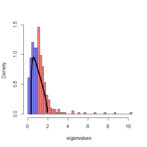
Figure 6 (c) is the histogram of the eigenvalues of $\mathbf{R}$ . The red bins are for the eigenvalues more than 1 and the blue bins are for the eigenvalues less than 1. The black solid curve is the density of Marčenko-Pastur distribution with index $p/n=0.16$ and scale $1-\lambda_{1}(\mathbf{R})/p=0.98$ . There is a bin-width such that the histogram fits the density well. The $GK^{\mathbf{R}}=0.39$ has 10% error from the estimated value $GK_{{0.16},0.02}=0.44$ . This may be related to Observation 3.14 (3).

Next, we consider 16 microarray datasets from [36]. Table 2 is the list of the author of a microarray dataset, $p/n$ , $\lambda_{1}(\mathbf{R})/p$ , $GK^{\mathbf{R}}$ , $GK_{p/n,\lambda_{1}(\mathbf{R})/p}$ , $CP^{\mathbf{R}}(.7)$ and $p$ , in the increasing order of $p/n$ . Here $p$ is the number of features and $n$ is the number of observations.

Table 2. DNA microarray datasets.

No.	Name	$p/n$	$\lambda_{1}(\mathbf{R})/p$	$GK^{\mathbf{R}}$	$GK_{p/n,\lambda_{1}(\mathbf{R})/p}$	$CP^{\mathbf{R}}(.7)$	$p$
1	Sorlie	5.4	.110	.16228	.18640	.05044	456
2	Gravier	17.3	.083	.05370	.05783	.01136	2905
3	Alon	32.3	.450	.03000	.03100	.00200	2000
4	Yeoh	50.9	.145	.01956	.01964	.00539	12625
5	Gordon	69.2	.087	.01436	.01444	.00367	12533
6	Tian	73.0	.089	.01362	.01370	.00554	12625
7	Shipp	92.6	.213	.01066	.01080	.00182	7129
8	Chiaretti	98.6	.181	.01006	.01014	.00190	12625
9	Golub	99.0	.149	.00996	.01010	.00351	7129
10	Pomeroy	118.8	.266	.00828	.00842	.00224	7128
11	West	145.5	.162	.00673	.00687	.00224	7129
12	Burczynski	175.5	.115	.00565	.00570	.00193	22283
13	Chin	188.3	.164	.00527	.00531	.00158	22215
14	Nakayama	212.2	.073	.00467	.00471	.00202	22283
15	Chowdary	214.2	.699	.00462	.00467	.00004	22283
16	Borovecki	718.8	.173	.00135	.00139	.00058	22283

Table 2 shows that $GK^{\mathbf{R}}>CP^{\mathbf{R}}(.7)$ and $GK^{\mathbf{R}}$ is nonincreasing in $p/n$ as Figure 5. Moreover, by Theorem 3.7 (4), $GK_{p/n,\lambda_{1}(\mathbf{R})/p}$ is $n/p$ because all datasets have $p/n$ more than $(1/\sqrt{1-\lambda_{1}(\mathbf{R})/p}+1)^{2}$ . Indeed, the empirical values $GK^{\mathbf{R}}$ are around $n/p$ for all datasets having $p/n$ sufficiently greater than the threshold $(1/\sqrt{1-\lambda_{1}(\mathbf{R})/p}+1)^{2}$ .

4.2. Datasets from economics

We consider the datasets of returns of $p$ S&P500 stocks for $n$ trading days. Laloux et al. [27] fitted the histogram of the correlation matrix $\mathbf{R}$ of such a dataset to the density function of a scaled Marčenko-Pastur distribution.

Table 3 is the list of $p/n$ , $\lambda_{1}(\mathbf{R})/p$ , $GK^{\mathbf{R}}$ , $GK_{p/n,\lambda_{1}(\mathbf{R})/p}$ , and $p=212$ S&P500 stocks of various periods, in the increasing order of $\lambda_{1}(\mathbf{R})/p.$

No	Period	$p/n$	$\lambda_{1}(\mathbf{R})/p$	$GK^{\mathbf{R}}$	$GK_{p/n,\lambda_{1}(\mathbf{R})/p}$	$p$
1	1993-01-04-1995-12-29	.2808	.1103	.3302	.3747	212
2	1993-01-04-2022-08-01	.0285	.3137	.1038	0	212
3	2012-08-01-2022-08-01	.0843	.4026	.0991	0	212
4	2005-01-04-2022-08-01	.0479	.4232	.0849	0	212
5	2005-01-04-2013-12-30	.0938	.4503	.0849	0	212

Table 3. The returns of S&P500 datasets.

$GK^{\mathbf{R}}$ is decreasing in $\lambda_{1}(\mathbf{R})/p$ in Table 3, as Observation 3.14 (2). It is worth noting that the estimator $GK_{p/n,\lambda_{1}(\mathbf{R})/p}$ is mostly 0.

Next, we consider similar but more categorized datasets. The return of a stock is more correlated with the return of a stock of the same industry classification sector than with the return of a stock of a different industry classification sector. Table 4 is the list of global industry classification standard (GICS) sector of S&P500, $p/n$ , $\lambda_{1}(\mathbf{R})/{p}$ , $GK^{\mathbf{R}}$ , $GK_{p/n,\lambda_{1}(\mathbf{R})/p}$ , and $p$ . All the periods are 2012-01-04/2022-12-31. Table 4 is ordered in the increasing order of $\lambda_{1}(\mathbf{R})/p$ . All the $p$ of Table 4 are smaller than the $p=212$ of Table 3, but some GICS sectors have larger $\lambda_{1}(\mathbf{R})/p$ . In Table 4, $GK^{\mathbf{R}}$ is decreasing if we omit the first line (Communication services, $p=19$ ), the fourth line (Consumer Staples, $p=23$ ), the seventh line (Material, $p=24$ ), the tenth line (Energy, $p=16$ ) from all the lines. Observation 3.14 (2) for Guttman-Kaiser criterion holds for $p\geq 28$ .

No	GICS	$p/n$	$\lambda_{1}(\mathbf{R})/p$	$GK^{\mathbf{R}}$	$p$
1	Communication Serv.	.0076	.3571	.2105	19
2	Consumer Discret.	.0207	.3843	.1538	52
3	Health Care	.0187	.3948	.1489	47
4	Consumer Staples	.0091	.4302	.1739	23
5	Information Tech.	.0246	.4648	.0968	62
6	Industrials	.0258	.4985	.0923	65
7	Materials	.0095	.4990	.1667	24
8	Real estate	.0119	.5819	.1000	30
9	Financials	.0250	.6086	.0794	63
10	Energy	.0064	.6872	.0625	16
11	Utilities	.0111	.6897	.0714	28

Table 4. The returns of S&P500 stocks per GICS.

The estimator $GK_{p/n,\lambda_{1}(\mathbf{R})/p}$ of $GK^{\mathbf{R}}$ in Table 3 and Table 4 are all 0 for $\lambda_{1}(\mathbf{R})/p>0.110$ . The estimator $GK_{p/n,\lambda_{1}(\mathbf{R})/p}=1-F_{p/n,1}\left(1/(1-\lambda_{1}(\mathbf{R})/p)\right)$ is $0$ if $p/n<1$ but $\lambda_{1}(\mathbf{R})/p<1$ is sufficiently large. The first author computed the time series of equi-correlations for the datasets, by employing GJR GARCH [13] with correlation structure being dynamic equicorrelation [10]. Then, $\lambda_{1}(\mathbf{R})/p$ is always larger than the time averages of the time series of the equi-correlation coefficient.

To detect the correlation structure from stock datasets (Table 3 and Table 4), we apply a hierarchical clustering algorithm to the sample correlation matrices $\mathbf{R}$ of the datasets, and then computed their color heat maps. We found that they are very different from the heat map Figure 6 of the correlation matrix of the binary MSA dataset. The correlation matrices of the stock returns have diagonal block structures. Moreover, the sizes of the GICS correlation matrices are small. By these, $GK^{\mathbf{R}}$ of the stock returns datasets may be discrepant from our estimator $GK_{p/n,\lambda(\mathbf{R})/p}$ .

Finally, we consider two household datasets in 2019 by area classification, from [38]. One is for the amount of assets per households and the other is for the average yearly income. These datasets have response variables: the amount of assets and liabilities per household and the average yearly income from the whole of Japan. Meanwhile, the explanatory variables are the amount of assets per households and the average yearly income from each of 66 regions in Japan. We can detect the multicollinearity [7, 23] by variance inflation factors (VIFs) [7, 23] of the explanatory variables. If all the explanatory variables are uncorrelated, then all the VIFs are equal to 1, but if severe multicollinearities exist, then the VIFs for some explanatory variables become very large [7, 23].

Name	$\min$ VIF	$R^{2}$	$\lambda_{1}(\mathbf{R})/p$	$GK^{\mathbf{R}}$	$p$	$p/n$
The amount of assets 2019	8.44 $\times 10^{2}$	1	.980	.015	66	.051
The average yearly income 2019	1.47 $\times 10^{4}$	1	.993	.015	66	.048

Table 5. The household datasets of 2019.

Table 5 is the list of name, $\min$ VIFs, the (adjusted) coefficient $R^{2}$ of determination, $\lambda_{1}(\mathbf{R})/p$ , $GK^{\mathbf{R}}$ , $p=66$ variables, and $p/n$ , in the increasing order of $\lambda_{1}(\mathbf{R})/p.$ Since $R^{2}=1$ for both datasets, we can assume that all the explanatory variables have the equi-correlation coefficient $\rho=1$ , which means $\lambda_{1}(\mathbf{R})/p$ is approximately 1. One of future work is to discuss the multicollinearity and other correlation structures [3, 6, 10, 12, 30, 33] among variables with the extreme eigenvalues and the bulk eigenvalues of datasets, by employing random matrix theory.

5. Conclusion

For assessing the (essential) dimensionality of empirical data, the Guttman-Kaiser criterion is a widely employed criterion. This rule may be the most used for retaining principal components and factors owing to its clarity, ease of implementation [11], and default stopping rule in statistical tools such as SPSS and SAS. In this paper, we have shown the scaling of Marčenko-Pastur distribution when a dataset is from an ENP and $0\leq\rho<1$ by the LSD of the sample correlation matrix. This scaling of Marčenko-Pastur distribution explains the “phase transitions” of Guttman-Kaiser criterion depending on whether $\rho=0$ or not as $n,p\to\infty,\ p/n\to c>0$ . Moreover, by Observation 3.14, we show the behavior of Guttman-Kaiser criterion where this criterion retains the small number of principal components or factors in small $c$ for $0<\rho<1$ and the limit of $GK^{\mathbf{R}}$ is 1/2 in $c\downarrow 0$ for $\rho=0$ . In high-dimensional statistics of various fields, when the number of variables are smaller than the size of a sample, a global correlation among the variables causes a perceptible global impact, even if the correlation is minute.

Acknowledgment

The authors are partially supported by Graduate School of Science, Tohoku University. The MSA dataset is kindly provided from Prof. A. A. Quadeer through the email correspondence with Prof. M. R. McKay on 22 September, 2022.

Appendix A Proofs of Theorem 3.11 and Theorem 3.12

Suppose that $\mathbf{M}$ is a positive real symmetric semi-definite matrix of order $p$ where all $p$ eigenvalues follow (23). For $k>0$ , the eigenvalues of matrix $k\mathbf{M}$ are (23) multiplied by $k$ because the eigenvalues of matrix $\mathbf{M}$ follows (23). Thus, for a random distribution function $G^{\mathbf{M}}$ defined by (24), $G^{k\mathbf{M}}(kx)=G^{\mathbf{M}}(x)$ for any $x\in\mathbb{R}$ . We represent $G^{\mathbf{M}}$ by using $x\vee 0:=\max(x,0)$ and the probability measure $\mu^{\mathbf{M}}$ corresponding to the distribution function $F^{\mathbf{M}}$ .

Lemma A.1.

\displaystyle G^{\mathbf{M}}(x)

\displaystyle=\frac{\int_{[0,x\vee 0]}\lambda\,d\mu^{\mathbf{M}}(\lambda)}{\int_{\mathbb{R}}\lambda\,d\mu^{\mathbf{M}}(\lambda)},\qquad(x\in\mathbb{R}).

Proof.

By (23), $\mu^{\mathbf{M}}\left((-\infty,0)\right)=0$ . Because $F^{\mathbf{M}}(x)=p^{-1}\sum_{i=1}^{p}\mathbf{1}_{\lambda_{i}\leq x}$ for all $x\in\mathbb{R}$ , $G^{\mathbf{M}}(x)=\sum_{\lambda_{i}\leq x}\lambda_{i}/\sum_{i=1}^{p}\lambda_{i}$ . Since ${\sum_{\lambda_{i}\leq x}\lambda_{i}}\leq{\sum_{\lambda_{i}\leq z}\lambda_{i}}$ for $x\leq z$ , $G^{\mathbf{M}}$ is nondecreasing. Since $[\lambda_{i},\,\infty)$ has a left endpoint, the right-continuity is clear from $G^{\mathbf{M}}$ . Moreover, $\lim_{x\to-\infty}G^{\mathbf{M}}(x)=0$ and $\lim_{x\to+\infty}G^{\mathbf{M}}(x)=1$ . Therefore $G^{\mathbf{M}}$ is indeed a random distribution function. ∎

Lemma A.2.

For $u\in(0,1)$ , $\min\set{\lambda_{i}}{\lambda_{i}>0,\ 1\leq i\leq p}\leq\left(G^{\mathbf{M}}\right)^{-}(u)\leq\lambda_{1}$ .

Proof.

By (24),

\displaystyle\left(G^{\mathbf{M}}\right)^{-}(u)=\inf\Set{x}{\sum_{\lambda_{i}>x}\lambda_{i}\big/\sum_{i=1}^{p}\lambda_{i}\leq 1-u}.

(25)

Because $\lambda_{1}$ is the largest eigenvalue of $\mathbf{M}$ , $\sum_{\lambda_{i}>\lambda_{1}}\lambda_{i}=0$ . By $0<u<1$ , $\lambda_{1}$ is an element of the set in the right side of (25). Hence, $\left(G^{\mathbf{M}}\right)^{-}(u)\leq\lambda_{1}$ . On the other hand, if $x=0$ and $x<\min_{1\leq i\leq p}\lambda_{i}$ , $\sum_{\lambda_{i}>x}\lambda_{i}/\sum_{i=1}^{p}\lambda_{i}=1$ . Thus, by $u\in(0,1)$ , whenever $\sum_{\lambda_{i}>x}\lambda_{i}\big/\sum_{i=1}^{p}\lambda_{i}\leq 1-u$ , $x\geq\min\set{\lambda_{i}}{\lambda_{i}>0,\ 1\leq i\leq p}$ . Therefore, $\min\set{\lambda_{i}}{\lambda_{i}>0,\ 1\leq i\leq p}\leq\left(G^{\mathbf{M}}\right)^{-}(u)\leq\lambda_{1}$ . ∎

In sequel, for $t\in(0,\,1)$ , we show that $\left(G^{\mathbf{M}}\right)^{-}(1-t)$ is a threshold for eigenvalues CPV rule retains. In Definition 3.10, we gave the representation of $CP_{c,\rho}$ with the complementary distribution function of $F_{c,1}$ and the quantile function of $G_{c,1}$ . Like this, but by replacing the subscripts with the superscripts $\mathbf{M}$ and by replacing $(1-t)/(1-\rho)$ with $1-t$ , we have the following representation of $CP^{\mathbf{M}}(t)$ :

Lemma A.3.

For any real symmetric positive semi-definite matrix $\mathbf{M}$ ,

CP^{\mathbf{M}}(t)=\overline{F^{\mathbf{M}}}(\left(G^{\mathbf{M}}\right)^{-}(1-t)),\qquad(0<t<1).

Proof.

Let $q=pCP^{\mathbf{M}}(t)$ . By $\sum_{\lambda_{i}>\lambda_{q+1}}\lambda_{i}\big/\sum_{i=1}^{p}\lambda_{i}\leq t$ and $\lambda_{q}>\lambda_{q+1}$ , (25) implies $\lambda_{q+1}\geq\left(G^{\mathbf{M}}\right)^{-}(1-t)$ . If $x<\lambda_{q+1}$ , then $\sum_{\lambda_{i}>x}\lambda_{i}\big/\sum_{i=1}^{p}\lambda_{i}>t$ by (25). Thus, $\lambda_{q+1}\leq\left(G^{\mathbf{M}}\right)^{-}(1-t).$ As a result, $\lambda_{q+1}=\left(G^{\mathbf{M}}\right)^{-}(1-t).$ Thus, by Definition 3.8, $CP^{\mathbf{M}}(t)=\frac{1}{p}\times\#\Set{i}{\lambda_{i}>\left(G^{\mathbf{M}}\right)^{-}(1-t)}=\overline{F^{\mathbf{M}}}(\left(G^{\mathbf{M}}\right)^{-}(1-t)).$ ∎

We can readily observe the following:

Lemma A.4.

$G_{c,\sigma^{2}}$ is a continuous distribution function which is strictly increasing on $(a_{\sigma^{2}}(c),b_{\sigma^{2}}(c))$ , and

\displaystyle G_{c,\sigma^{2}}(x)=\frac{\int_{[0,\,x\vee 0]}\lambda d\mu_{c,\sigma^{2}}(\lambda)}{\int_{\mathbb{R}}\lambda d\mu_{c,\sigma^{2}}(\lambda)},\qquad(x\in\mathbb{R}).

Moreover, $G_{c,\sigma^{2}}(x)=G_{c,1}(x/\sigma^{2})$ for all $x\in\mathbb{R}$ .

Lemma A.5.

The function $G_{c,\sigma^{2}}$ restricted to an open interval $J=(a_{\sigma^{2}}(c),\,b_{\sigma^{2}}(c))$ has $\left(G_{c,\sigma^{2}}\right)^{-}$ as the inverse function. Moreover, $\left(G_{c,\sigma^{2}}\right)^{-}$ is a continuous, strictly increasing function from the unit open interval $(0,1)$ to $J$ .

Proof.

By Lemma A.4, $G_{c,\sigma^{2}}$ is strictly increasing on $J$ . Let $\tilde{x}\in J$ . Then $\left(G_{c,\sigma^{2}}\right)^{-}(G_{c,\sigma^{2}}(\tilde{x}))=\tilde{x}$ by $\left(G_{c,\sigma^{2}}\right)^{-}(G_{c,\sigma^{2}}(\tilde{x}))=\inf\Set{x}{G_{c,\sigma^{2}}(x)\geq G_{c,\sigma^{2}}(\tilde{x})}$ . For any $t\in(0,1)$ , $\left(G_{c,\sigma^{2}}\right)^{-}(t)=\inf\Set{x}{G_{c,\sigma^{2}}(x)=t}$ . Since $G_{c,\sigma^{2}}$ is continuous function, $G_{c,\sigma^{2}}(\left(G_{c,\sigma^{2}}\right)^{-}(t))=t$ . Hence, $\left(G_{c,\sigma^{2}}\right)^{-}$ is the inverse function of $G_{c,\sigma^{2}}$ restricted to $J$ , and $\left(G_{c,\sigma^{2}}\right)^{-}$ is a continuous, strictly increasing function from $(0,1)$ to $J$ .∎

Lemma A.6.

For $c,\sigma^{2},k>0$ , $z\in\mathbb{R}$ ,

(1)

$\left(kG_{c,\sigma^{2}}\right)^{-}\left(z\right)=\left(G_{c,\sigma^{2}}\right)^{-}\left({z}/{k}\right).$
(2)

$\overline{F_{c,\sigma^{2}}}\left(\left(G_{c,\sigma^{2}}\right)^{-}\left(z\right)\right)=\overline{F_{c,1}}\left(\left(G_{c,1}\right)^{-}\left(z\right)\right).$
(3)

$\overline{F_{c,1}}\left(\left(G_{c,1}\right)^{-}(t)\right)\in(0,\,1)$ , if $t\in(0,\,1)$ .

Proof.

(1) ${\left(kG_{c,\sigma^{2}}\right)^{-}(z)}=\inf\Set{x\in\mathbb{R}}{kG_{c,\sigma^{2}}(x)\geq z}$ . By $k>0$ , it is equal to $\inf\Set{x\in\mathbb{R}}{G_{c,\sigma^{2}}(x)\geq z/k}=\left(G_{c,\sigma^{2}}\right)^{-}\left(z/k\right).$

(2) $\overline{F_{c,\sigma^{2}}}\left(\left(G_{c,\sigma^{2}}\right)^{-}\left(z\right)\right)=\overline{F_{c,1}}\left(\frac{1}{\sigma^{2}}{\left(G_{c,\sigma^{2}}\right)^{-}\left(z\right)}\right)$ . By the definition of the quantile function, $\left(G_{c,\sigma^{2}}\right)^{-}\left(z\right)/\sigma^{2}=\inf\Set{x}{G_{c,\sigma^{2}}(\sigma^{2}x)\geq z}$ which is equal to $\left(G_{c,1}\right)^{-}\left(z\right)$ . Thus, $\overline{F_{c,\sigma^{2}}}\left(\left(G_{c,\sigma^{2}}\right)^{-}(z)\right)=\overline{F_{c,1}}\left(\left(G_{c,1}\right)^{-}(z)\right)$ .

(3) By Lemma A.5, we have $\left(G_{c,1}\right)^{-}:(0,1)\to(a_{1}(c),b_{1}(c))$ . Because $\overline{F_{c,1}}$ restricted to $(a_{1}(c),\,b_{1}(c))$ is a strictly decreasing function to $(0,\,1)$ , it follows that $\overline{F_{c,1}}\left(\left(G_{c,1}\right)^{-}(t)\right)\in(0,1)$ for $t\in(0,\,1)$ . ∎

The following proposition is Arzelà’s dominated convergence theorem [28]. By this, we prove that the distribution function $G^{\mathbf{R}}$ ( $G^{\mathbf{S}}$ , resp.) almost surely converges pointwise to a defective distribution function $(1-\rho)G_{c,1-\rho}$ ( $(1-\rho)G_{c,\sigma^{2}(1-\rho)}$ , resp.).

Proposition A.7 ([28, Theorem A]).

Let $\{f_{n}\}$ be a sequence of Riemann-integrable functions defined on a bounded and closed interval $[a,\,b]$ , which converges on $[a,\,b]$ to a Riemann-integrable function $f$ . If there exists a constant $M>0$ satisfying $|f_{n}(x)|\leq M$ for all $x\in[a,\,b]$ and for all $n$ , then $\lim_{n\to\infty}\int_{a}^{b}\left|f_{n}(x)-f(x)\right|dx=0$ . In particular,

\lim_{n\to\infty}\int_{a}^{b}f_{n}(x)dx=\int_{a}^{b}\lim_{n\to\infty}f_{n}(x)dx=\int_{a}^{b}f(x)dx.

Lemma A.8.

Suppose $X_{1},\ldots,X_{n}\stackrel{{\scriptstyle\mbox{\rm i.{}i.{}d.{}}}}{{\sim}}\mathrm{N}(\bm{\mu},\,\mathbf{D}\mathbf{C}(\rho)\mathbf{D})$ for $0\leq\rho<1$ . Suppose $n,p\to\infty$ with $p/n\to c>0$ . Then, it holds almost surely that for any $x\in\mathbb{R}$ ,

(1)

$G^{\mathbf{R}}(x)\to(1-\rho)G_{c,1-\rho}(x)$ ,
(2)

$G^{\mathbf{S}}(x)\to(1-\rho)G_{c,\sigma^{2}(1-\rho)}(x)$ for $\bm{\mu}=\bm{0}$ and $\mathbf{D}=\sigma\mathbf{I}$ with $\sigma>0$ .

Proof.

For a symmetric positive semi-definite $\mathbf{M}$ , we know that $\int_{[0,x\vee 0]}\lambda d\mu^{\mathbf{M}}(\lambda)=\int_{0}^{x\vee 0}\mu^{\mathbf{M}}\left(\set{\lambda}{f(\lambda)>h}\right)dh$ for $f:\mathbb{R}\to\mathbb{R}$ such that $f(\lambda)$ be $\lambda$ for $0<\lambda\leq x$ and 0 otherwise. For $h\geq 0$ , $f(\lambda)>h$ if and only if $h<\lambda\leq x$ . Then, $\mu^{\mathbf{M}}\left(\set{\lambda}{f(\lambda)>h}\right)$ $=F^{\mathbf{M}}(x)-F^{\mathbf{M}}(h)$ for $0\leq h<x$ , and 0 otherwise. Similarly, $\mu_{c,\sigma^{2}}(\set{\lambda}{f(\lambda)>h})$ $=F_{c,\sigma^{2}}(x)-F_{c,\sigma^{2}}(h)$ for $0\leq h<x$ , and 0 otherwise.

(1) Since the sample correlation matrices $\mathbf{R}$ are invariant under scaling of variables, we can write $\mathbf{D}=\mathbf{I}$ without loss of generality. Moreover, we can assume that $\bm{\mu}=\bm{0}$ because $\mathbf{R}$ is invariant under sifting. Because $\int_{\mathbb{R}}\lambda\,d\mu^{\mathbf{R}}(\lambda)=\Tr\mathbf{R}/p=1$ and $\int_{\mathbb{R}}\lambda d\mu_{c,1-\rho}(\lambda)=1-\rho$ , the denominator of $G^{\mathbf{R}}(x)$ in Lemma A.1 $(G_{c,1-\rho}(x)$ in Lemma A.4, resp.) is 1 ( $1-\rho$ , resp.) for all $x\in\mathbb{R}$ . By this, the representation of Lebesgue integral with a Riemann integral, Lemma A.1 and Lemma A.4, for all positive integer $p$ and $x\in\mathbb{R}$ ,

		$\displaystyle\left\|G^{\mathbf{R}}(x)-(1-\rho)G_{c,1-\rho}(x)\right\|=\left\|\int_{[0,x\vee 0]}\lambda d\mu^{\mathbf{R}}(\lambda)-\int_{[0,x\vee 0]}\lambda d\mu_{c,1-\rho}(\lambda)\right\|$
		$\displaystyle=\left\|\int_{0}^{x\vee 0}(F^{\mathbf{R}}(x)-F^{\mathbf{R}}(h))-(F_{c,1-\rho}(x)-F_{c,1-\rho}(h))dh\right\|$
		$\displaystyle\leq\|x\vee 0\|\|F^{\mathbf{R}}(x)-F_{c,1-\rho}(x)\|+\left\|\int_{0}^{x\vee 0}F^{\mathbf{R}}(h)-F_{c,1-\rho}(h)dh\right\|.$		(26)

By Theorem 2.11, for all $c>0$ , it holds almost surely that for any $x\neq 0$ we have $F^{\mathbf{R}}(x)\to F_{c,1-\rho}(x)$ . Thus, for any $c>0$ , it holds almost surely that for any $x$ , the first term of the right side of (26) converges to 0. Define two functions $\tilde{F}^{\mathbf{R}}:[0,\,x]\to[0,\,1]$ and $\tilde{F}_{c,1-\rho}:[0,\,x]\to[0,\,1]$ as follows: $\tilde{F}^{\mathbf{R}}(h)=0\ (h=0)$ ; $F^{\mathbf{R}}(h)\ (0<h\leq x)$ ; and $\tilde{F}_{c,1-\rho}(h)=0\ (h=0)$ ; $F_{c,1-\rho}(h)\ (0<h\leq x)$ . The four functions $\tilde{F}^{\mathbf{R}}$ , $F^{\mathbf{R}}$ , $\tilde{F}_{c,1-\rho}$ , and $F_{c,1-\rho}$ are Riemann-integrable over $[0,x]$ , because they are nondecreasing. Moreover, $\int_{0}^{x\vee 0}\tilde{F}^{\mathbf{R}}(h)dh=\int_{0}^{x\vee 0}F^{\mathbf{R}}(h)dh$ , and $\int_{0}^{x\vee 0}\tilde{F}_{c,1-\rho}(h)dh=\int_{0}^{x\vee 0}F_{c,1-\rho}(h)dh$ . For any $h\in[0,x]$ , $|\tilde{F}^{\mathbf{R}}(h)|\leq 1$ . By Theorem 2.11, for all $c>0$ , it holds almost surely that $\tilde{F}^{\mathbf{R}}$ converges pointwise to $\tilde{F}_{c,1-\rho}$ . Hence, by Arzelà’s dominated convergence theorem [28], it holds almost surely that

\int_{0}^{x\vee 0}F^{\mathbf{R}}(h)dh=\int_{0}^{x\vee 0}\tilde{F}^{\mathbf{R}}(h)dh\to\int_{0}^{x\vee 0}\tilde{F}_{c,1-\rho}(h)dh=\int_{0}^{x\vee 0}F_{c,1-\rho}(h)dh.

Thus, the second term of the right side of (26) converges almost surely to 0. Therefore, for all $c>0$ , almost surely $G^{\mathbf{R}}$ converges pointwise to $(1-\rho)G_{c,1-\rho}$ .

(2) By a similar argument to (26), $\left|\int_{[0,x\vee 0]}\lambda d\mu^{\mathbf{S}}(\lambda)-\int_{[0,x\vee 0]}\lambda d\mu_{c,\sigma^{2}(1-\rho)}(\lambda)\right|$ is

		$\displaystyle=\left\|(x\vee 0)(F^{\mathbf{S}}(x)-F_{c,\sigma^{2}(1-\rho)}(x))+\int_{0}^{x\vee 0}(F_{c,\sigma^{2}(1-\rho)}(h)-F^{\mathbf{S}}(h))dh\right\|$
		$\displaystyle\leq\|x\vee 0\|\|F^{\mathbf{S}}(x)-F_{c,\sigma^{2}(1-\rho)}(x)\|+\left\|\int_{0}^{x\vee 0}F^{\mathbf{S}}(h)-F_{c,\sigma^{2}(1-\rho)}(h)dh\right\|.$		(27)

By Theorem 2.7, for all $c>0$ , almost surely, for any $x\in\mathbb{R}$ , the first term of (27) converges to 0. Define two functions $\tilde{F}^{\mathbf{S}}:[0,\,x]\to[0,\,1]$ and $\tilde{F}_{c,\sigma^{2}(1-\rho)}:[0,\,x]\to[0,\,1]$ as follows: $\tilde{F}^{\mathbf{S}}(h)=0\ (h=0)$ ; $F^{\mathbf{S}}(h)\ (0<h\leq x)$ ; and $\tilde{F}_{c,\sigma^{2}(1-\rho)}(h)=0\ (h=0)$ ; $F_{c,\sigma^{2}(1-\rho)}(h)\ (0<h\leq x)$ . Note that $\tilde{F}^{\mathbf{S}}$ , $F^{\mathbf{S}}$ , $\tilde{F}_{c,\sigma^{2}(1-\rho)}$ , and $F_{c,\sigma^{2}(1-\rho)}$ are Riemann-integrable over $[0,x\vee 0]$ , because they are nondecreasing. Moreover, $\int_{0}^{x\vee 0}\tilde{F}^{\mathbf{S}}(h)dh=\int_{0}^{x\vee 0}F^{\mathbf{S}}(h)dh$ , and $\int_{0}^{x\vee 0}\tilde{F}_{c,\sigma^{2}(1-\rho)}(h)dh=\int_{0}^{x\vee 0}F_{c,\sigma^{2}(1-\rho)}(h)dh$ . For any $h\in[0,x]$ , $|\tilde{F}^{\mathbf{S}}(h)|\leq 1$ . By Theorem 2.7, for all $c>0$ , almost surely, $\tilde{F}^{\mathbf{S}}$ converges pointwise to $\tilde{F}_{c,\sigma^{2}(1-\rho)}$ . Hence, by Arzelà’s dominated convergence theorem [28],

\int_{0}^{x\vee 0}F^{\mathbf{S}}(h)dh=\int_{0}^{x\vee 0}\tilde{F}^{\mathbf{S}}(h)dh

converges almost surely to

\int_{0}^{x\vee 0}\tilde{F}_{c,\sigma^{2}(1-\rho)}(h)dh=\int_{0}^{x\vee 0}F_{c,\sigma^{2}(1-\rho)}(h)dh.

As a result, the second term of the right side of (27) converge almost surely to 0. Thus, for all $c>0$ , almost surely

\int_{[0,x\vee 0]}\lambda d\mu^{\mathbf{S}}(\lambda)\to\int_{[0,x\vee 0]}\lambda d\mu_{c,\sigma^{2}(1-\rho)}(\lambda),\qquad(x\in\mathbb{R}).

Besides, $\int_{\mathbb{R}}\lambda d\mu^{\mathbf{S}}(\lambda)\to\sigma^{2}$ by Lemma 2.9. Therefore, for all $c>0$ , almost surely, for all $x\in\mathbb{R}$ ,

\displaystyle G^{\mathbf{S}}(x)=\frac{\int_{[0,x\vee 0]}\lambda d\mu^{\mathbf{S}}(\lambda)}{\int_{\mathbb{R}}\lambda d\mu^{\mathbf{S}}(\lambda)}\to\frac{\int_{[0,x\vee 0]}\lambda d\mu_{c,\sigma^{2}(1-\rho)}(\lambda)}{\sigma^{2}}=(1-\rho)G_{c,\sigma^{2}(1-\rho)}(x),

as desired. ∎

Proposition A.9 ([9]).

Suppose $f:\mathbb{R}\to\mathbb{R}$ is nondecreasing, and let $f(-\infty)=\lim_{x\downarrow-\infty}f(x)$ and $f(\infty)=\lim_{x\uparrow\infty}f(x)$ . Let $x,y\in\mathbb{R}$ . Then, $f(x)\geq y$ implies $x\geq f^{-}(y).$ The other implication holds if $f$ is right-continuous. Furthermore, $f(x)<y$ implies $x\leq f^{-}(y).$

Lemma A.10.

If a distribution function $H_{n}$ weakly converges to a defective distribution function $H$ , then $H_{n}^{-}(t)$ converges to $H^{-}(t)$ for any continuity point $t$ of $H^{-}$ .

Proof.

This lemma is Theorem 2A [32] when $H$ is not defective. We use Theorem 2A [32] to prove this lemma. Let $0<t<1$ be a continuity point of $H^{-}$ . Then one can pick a sequence $\epsilon_{k}$ that converges to 0 such that $H^{-}(t)-\epsilon_{k}$ and $H^{-}(t)+\epsilon_{k}$ are continuity points of $H$ and $H(H^{-}(t)-\epsilon_{k})<t<H(H^{-}(t)+\epsilon_{k}),$ for each fixed $k$ . By the assumption, $N_{k}$ may be chosen such that $H_{n}(H^{-}(t)-\epsilon_{k})<t<H_{n}(H^{-}(t)+\epsilon_{k}),$ for any $n>N_{k}$ . Therefore, by Proposition A.9, for $n\geq N_{k}$ , $H^{-}(t)-\epsilon_{k}\leq H_{n}^{-}(t)\leq H^{-}(t)+\epsilon_{k}.$ $H_{n}^{-}(t)\to H^{-}(t)$ can be deduced. ∎

Lemma A.11.

(1)

$\left(G^{\mathbf{R}}\right)^{-}(u)\to\left((1-\rho)G_{c,1-\rho}\right)^{-}(u)$ , and
(2)

$\left(G^{\mathbf{S}}\right)^{-}(u)\to\left((1-\rho)G_{c,\sigma^{2}(1-\rho)}\right)^{-}(u)$ for $\bm{\mu}=\bm{0}$ and $\mathbf{D}=\sigma\mathbf{I}$ with $\sigma>0$ .

Proof.

By Lemma A.5, both of $\left((1-\rho)G_{c,1-\rho}\right)^{-}$ and $\left((1-\rho)G_{c,\sigma^{2}(1-\rho)}\right)^{-}$ are continuous at $u\in(0,\,1-\rho].$ Therefore, the conclusion follows from Lemma A.8 and Lemma A.10. ∎

Proof of Theorem 3.11. Let $\mathbf{M}$ be $\mathbf{R}$ or $\mathbf{S}$ and let $\lambda_{1}\geq\cdots\geq\lambda_{p}$ be the eigenvalues of $\mathbf{M}$ .

(1) By Lemma A.2, $\left(G^{\mathbf{R}}\right)^{-}\left({1-t}\right)>0$ . Therefore, $\left(G^{\mathbf{R}}\right)^{-}\left({1-t}\right)$ is a continuity point of $F_{c,1-\rho}$ for any $c>0$ . Thus, by Lemma A.3 and Theorem 2.11, for all $c>0$ , it holds almost surely that for any $t\in[\rho,\,1)$ ,

\displaystyle\begin{aligned} &CP^{\mathbf{R}}(t)-\overline{F_{c,1-\rho}}\left(\left(G^{\mathbf{R}}\right)^{-}\left({1-t}\right)\right)\\ &=\overline{F^{\mathbf{R}}}\left(\left(G^{\mathbf{R}}\right)^{-}\left({1-t}\right)\right)-\overline{F_{c,1-\rho}}\left(\left(G^{\mathbf{R}}\right)^{-}\left({1-t}\right)\right)\to 0.\end{aligned}

(28)

By Lemma A.11 and Lemma A.6, we have $\left(G^{\mathbf{R}}\right)^{-}(1-t)\mathrel{\stackrel{{\scriptstyle a.s.}}{{\to}}}\left((1-\rho)G_{c,1-\rho}\right)^{-}$ $(1-t)=\left(G_{c,1-\rho}\right)^{-}\left(s\right)$ , where $s=({1-t})/({1-\rho}).$ By the premise $0<\rho\leq t<1$ , $0<s\leq 1$ , $\left(G_{c,1-\rho}\right)^{-}\left(s\right)=\inf\set{x}{G_{c,1-\rho}(x)\geq s}$ is positive and finite. Therefore, $\left(G_{c,1-\rho}\right)^{-}\left(s\right)$ is a continuous point of $\overline{F_{c,1-\rho}}.$ By continuous mapping theorem [39, Theorem 2.3], it holds almost surely that for any $t\in[\rho,\,1)$ ,

\overline{F_{c,1-\rho}}\left(\left(G^{\mathbf{R}}\right)^{-}\left({1-t}\right)\right)\to\overline{F_{c,1-\rho}}\left(\left(G_{c,1-\rho}\right)^{-}\left(s\right)\right).

By this and (28), it holds almost surely that for any $t\in[\rho,1)$ , $CP^{\mathbf{R}}(t)\to\overline{F_{c,1-\rho}}$ $\left(\left(G_{c,1-\rho}\right)^{-}\left(s\right)\right)=\overline{F_{c,1}}\left(\left(G_{c,1}\right)^{-}\left(s\right)\right)=CP_{c,\rho}(t)$ .

(2) We prove that, it holds almost surely that for any $t\in[\rho,1)$ , $CP^{\mathbf{S}}(t)\to\overline{F_{c,\sigma^{2}(1-\rho)}}\left(\left(G_{c,\sigma^{2}(1-\rho)}\right)^{-}\left(s\right)\right)$ . It can be similarly proved as the convergence of $CP^{\mathbf{R}}(t)$ by using Theorem 2.7 instead of Theorem 2.11. By Lemma A.6,

\overline{F_{c,\sigma^{2}(1-\rho)}}\left(\left(G_{c,\sigma^{2}(1-\rho)}\right)^{-}\left(s\right)\right)=\overline{F_{c,1}}\left(\left(G_{c,1}\right)^{-}\left(s\right)\right).

Thus, it holds almost surely that for any $t\in[\rho,1)$ , $CP^{\mathbf{S}}(t)\to CP_{c,\rho}(t)$ .

Proof of Theorem 3.12. The proof for the assertion of $\mathbf{R}$ ( $\mathbf{S}$ , resp.) is that of Theorem 3.11 except that $\rho$ should be 0, $t\in[\rho,1)$ should be $t\in(0,1)$ , and Theorem 2.11 should be Proposition 2.2 (Proposition 2.1, resp.).

REFERENCES

[1] Akama, Y., “Correlation matrix of equi-correlated normal population: fluctuation of the largest eigenvalue, scaling of the bulk eigenvalues, and stock market”, Preprint, (2022).
[2] Anderson, G. W., Guionnet, A. and Zeitouni, O., An introduction to random matrices, Cambridge University Press, Cambridge, 2010.
[3] Bai, Z. and Zhou, W., “Large sample covariance matrices without independence structures in columns”, Stat. Sin. 18(2) (2008), 425–442.
[4] Bai, Z. D., “Methodologies in spectral analysis of large dimensional random matrices, a review”, Stat. Sin. 9(3) (1999), 611–662.
[5] Bai, Z. D. and Yin, Y. Q., “Limit of the smallest eigenvalue of a large dimensional sample covariance matrix”, Ann. Probab. 21(3) (1993), 1275–1294.
[6] Bryson, J., Vershynin, R. and Zhao, H., “Marchenko–Pastur law with relaxed independence conditions”, Random Matrices Theory Appl (2021), 2150040.
[7] Chatterjee, S. and Hadi, A. S., Regression analysis by example, 4th ed. John Wiley & Sons, Hoboken, 2006.
[8] Dahirel, V., Shekhar, K., Pereyra, F., Miura, T., Artyomov, M., Talsania, S., Allen, T. M., Altfeld, M., Carrington, M., Irvine, D. J. et al., “Coordinate linkage of HIV evolution reveals regions of immunological vulnerability”, Proc. Natl. Acad. Sci. U.S.A. 108(28) (2011), 11530–11535.
[9] Embrechts, P. and Hofert, M., “A note on generalized inverses”, Math. Oper. Res. 77(3) (2013), 423–432.
[10] Engle, R. and Kelly, B., “Dynamic equicorrelation”, J. Bus. Econ. Stat. 30(2) (2012), 212–228.
[11] Fabrigar, L. R. and Wegener, D. T., Exploratory factor analysis, Oxford University Press, UK, 2011.
[12] Fan, J. and Jiang, T., “Largest entries of sample correlation matrices from equi-correlated normal populations”, Ann. Probab. 47(5) (2019), 3321–3374.
[13] Glosten, L. R., Jagannathan, R. and Runkle, D. E., “On the relation between the expected value and the volatility of the nominal excess return on stocks”, J. Finance 48(5) (1993), 1779–1801.
[14] Götze, F. and Tikhomirov, A., “Rate of convergence in probability to the Marchenko-Pastur law”, Bernoulli 10(3) (2004), 503–548.
[15] Götze, F. and Tikhomirov, A., “The rate of convergence of spectra of sample covariance matrices”, Theory Probab. Its Appl. 54(1) (2010), 129–140.
[16] Guttman, L., “Some necessary conditions for common-factor analysis”, Psychometrika 19(2) (1954), 149–161.
[17] Halabi, N., Rivoire, O., Leibler, S. and Ranganathan, R., “Protein sectors: evolutionary units of three-dimensional structure”, Cell 138(4) (2009), 774–786.
[18] Harman, H. H., Modern factor analysis, 3rd ed. University of Chicago press, Chicago, 1976.
[19] Huber, P. J. and Ronchetti, E. M., Robust statistics, 2nd ed. vol. 523. John Wiley & Sons, Hoboken, 2004.
[20] Husnaqilati, A., “Limiting spectral distribution of random matrices from equi-correlated normal population”, Preprint, (2022).
[21] Jackson, J. E., A user’s guide to principal components, vol. 587. John Wiley & Sons, Hoboken, 1991.
[22] Jiang, T., “The limiting distributions of eigenvalues of sample correlation matrices”, Sankhyā: The Indian Journal of Statistics (2003-2007) 66(1) (2004), 35–48.
[23] Jolliffe, I. T., Principal component analysis, 2nd ed. Springer, New York, 2002.
[24] Kaiser, H. F., “The application of electronic computers to factor analysis”, Educ. Psychol. Meas. 20(1) (1960), 141–151.
[25] Kaiser, H. F., “A measure of the average intercorrelation”, Educ. Psychol. Meas. 28(2) (1968), 245–247.
[26] Kaiser, H. F., “On Cliff’s formula, the Kaiser-Guttman rule, and the number of factors”, Percept. Mot. Ski. 74(2) (1992), 595–598.
[27] Laloux, L., Cizeau, P., Potters, M. and Bouchaud, J., “Random matrix theory and financial correlations”, Int. J. Theor. Appl. Finance. 3(3) (2000), 391–397.
[28] Luxemburg, W. A. J., “Arzela’s dominated convergence theorem for the Riemann integral”, Am. Math. Mon. 78(9) (1971), 970–979.
[29] Marčenko, V. A. and Pastur, L. A., “Distribution of eigenvalues for some sets of random matrices”, Mat USSR-Sborn 1(4) (1967), 457–483.
[30] Morales-Jimenez, D., Johnstone, I. M., McKay, M. R. and Yang, J., “Asymptotics of eigenstructure of sample correlation matrices for high-dimensional spiked models”, Stat. Sin. 31(2) (2021), 571–601.
[31] Mulaik, S. A., Foundations of factor analysis, 2nd ed. CRC press, Boca Raton, 2010.
[32] Parzen, E., “Quantile functions, convergence in quantile, and extreme value distribution theory”, Technical Report No. B-3, Texas A & M University, Institute of Statistics (1980).
[33] Peres-Neto, P. R., Jackson, D. A. and Somers, K. M., “How many principal components? Stopping rules for determining the number of non-trivial axes revisited”, Comput. Stat. Data Anal. 49(4) (2005), 974–997.
[34] Quadeer, A. A., Louie, R. H., Shekhar, K., Chakraborty, A. K., Hsing, I. and McKay, M. R., “Statistical linkage analysis of substitutions in patient-derived sequences of genotype 1a hepatitis C virus nonstructural protein 3 exposes targets for immunogen design”, J. Virol. 88(13) (2014), 7628–7644.
[35] Quadeer, A. A., Morales-Jimenez, D. and McKay, M. R., “Co-evolution networks of HIV/HCV are modular with direct association to structure and function”, PLOS Comput. Biol. 14(9) (2018), 1–29.
[36] Ramey, J., “Datamicroarray”, R package version 1.14.4. (2013).
[37] Silverstein, J. W., “Strong convergence of the empirical distribution of eigenvalues of large dimensional random matrices”, J. Multivar. Anal. 55(2) (1995), 331–339.
[38] Statistics Bureau, Ministry of Internal Affairs and Communications., “Statistics Bureau home page/national survey of family income, consumption and wealth”, https://www.stat.go.jp/english/data/zenkokukakei/index.htm.
[39] Van der Vaart, A. W., Asymptotic statistics, vol. 3. Cambridge University Press, Cambridge, 2000.
[40] Yao, J., Zheng, S. and Bai, Z. D., Sample covariance matrices and high-dimensional data analysis. Cambridge University Press, New York, 2015.
[41] Yeomans, K. A. and Golder, P. A., “The Guttman-Kaiser criterion as a predictor of the number of common factors”, J. R. Stat. Soc. 31(3) (1982), 221–229.
[42] Zwick, W. R. and Velicer, W. F., “Comparison of five rules for determining the number of components to retain”, Psychol. Bull. 99(3) (1986), 432–442.

		$\displaystyle\left\|G^{\mathbf{R}}(x)-(1-\rho)G_{c,1-\rho}(x)\right\|=\left\|\int_{[0,x\vee 0]}\lambda d\mu^{\mathbf{R}}(\lambda)-\int_{[0,x\vee 0]}\lambda d\mu_{c,1-\rho}(\lambda)\right\|$
		$\displaystyle=\left\|\int_{0}^{x\vee 0}(F^{\mathbf{R}}(x)-F^{\mathbf{R}}(h))-(F_{c,1-\rho}(x)-F_{c,1-\rho}(h))dh\right\|$
		$\displaystyle\leq\|x\vee 0\|\|F^{\mathbf{R}}(x)-F_{c,1-\rho}(x)\|+\left\|\int_{0}^{x\vee 0}F^{\mathbf{R}}(h)-F_{c,1-\rho}(h)dh\right\|.$		(26)