Method for solving inverse spectral problems on quantum star graphs
Abstract
A new method for solving inverse spectral problems on quantum star graphs is proposed. The method is based on Neumann series of Bessel functions representations for solutions of Sturm-Liouville equations. The representations admit estimates for the series remainders which are independent of the real part of the square root of the spectral parameter. This feature makes them especially useful for solving direct and inverse spectral problems requiring calculation of solutions on large intervals in the spectral parameter. Moreover, the first coefficient of the representation is sufficient for the recovery of the potential.
The method for solving the inverse spectral problem on the graph consists in reducing the problem to a two-spectra inverse Sturm-Liouville problem on each edge. Then a system of linear algebraic equations is derived for computing the first coefficient of the series representation for the solution on each edge and hence for recovering the potential. The proposed method leads to an efficient numerical algorithm that is illustrated by a number of numerical tests.
1 Introduction
Under quantum graphs or, in other words, differential equation networks we understand differential operators on metric graphs coupled by certain vertex matching conditions. Network-like structures play a fundamental role in many problems of science and engineering. The classical problem here that comes from applications is the problem of oscillations of the flexible structures made of strings, beams, cables, and struts. These models describe bridges, space-structures, antennas, transmission-line posts and other typical objects of civil engineering. Quantum graphs arise also as natural models of various phemonema in chemistry (free-electron theory of conjugated molecules), biology (genetic networks, dendritic trees), geophysics, environmental science, decease control, and even in Internet (Internet or network tomography). In physics, interest to quantum graphs arose, in particular, from applications to nano-electronics and quantum waveguides. On the other hand, quantum graph theory gives rise to numerous challenging problems related to many areas of mathematics from combinatorics to PDE and spectral theory. A number of surveys and collections of papers on quantum graphs appeared last years, and the first books on this topic by Berkolaiko and Kuchment [9], Mugnolo [21] and Kurasov [17] contain excellent lists of references.
Inverse spectral theory of network-like structures is an important part of the rapidly developing area of applied mathematics — analysis on graphs. The known results in this direction concern almost exclusively trees, i.e. graphs without cycles, see e.g. [18, 24, 8, 6, 7, 4].
To date, there are few papers containing numerical results for inverse problems on graphs, all of them concern only very simple trees [8, 3]. It is known that the problems of space discretization of differential equations on metric graphs turn out to be very difficult, and even the forward boundary value problems on graphs contain a lot of numerical challenges (see, e.g. [2]).
In the present work we develop a new method for solving inverse spectral problems on compact quantum star graphs that leads to efficient numerical algorithms. This method is based on Neumann series of Bessel functions representations for solutions of Sturm-Liouville equations. The method was proposed in [14] and successfully applied to solving direct and inverse spectral problems on intervals and the semiaxis in [13]. Here we extend this method to the inverse spectral problem for the Schrödinger equation on star graphs.
The Neumann series of Bessel functions representations for solutions of Sturm-Liouville equations,
possess two remarkable features which make them especially convenient for solving inverse problems. The remainders of the series admit -independent bounds for , and the potential of the equation can be recovered from the very first coefficient of the series. The first feature allows us to work with the approximate solutions on very large intervals in , and the second implies that computationally satisfactory results require considering a reduced number of the terms of the series which eventually results in a reduced number of linear algebraic equations which should be solved in each step.
The method consists of the following steps. First, using the given spectral data we compute coefficients of the series representations for solutions satisfying the homogeneous Dirichlet condition at the boundary vertices and for their derivatives at the end point of each edge, which is associated with the common vertex of the star graph. This first step allows us to split the problem on the graph into separate problems on each edge. Second, the set of coefficients for the series representation of the solution, evaluated at the end point of the interval allows us to compute the Dirichlet-Dirichlet eigenvalues of the potential on each edge. Moreover, the first feature of the series representations implies that if necessary hundreds of the eigenvalues can be computed with uniform accuracy, and for this few coefficients of the series representations are sufficient. Next, the knowledge of the Dirichlet-Dirichlet eigenvalues allows us to compute the important parameter (half of the integral of the potential) that is necessary for computing the Dirichlet-Neumann eigenvalues, for which, besides the parameter, the coefficients from the series representation of the derivative of the solution are used.
Thus, the inverse spectral problem on a graph is reduced to a two spectra inverse Sturm-Liouville problem on each edge. Results on the uniqueness and solvability of the two spectra problem are well known and can be found, e.g., in [11], [20], [23], [25]. For this problem we propose a method which again involves the Neumann series of Bessel functions representations for solutions and their derivatives. It allows us to compute multiplier constants [10] relating the Dirichlet-Neumann eigenfunctions associated with the same eigenvalues but normalized at the opposite endpoints of the interval. This leads to a system of linear algebraic equations for the coefficients of their series representations already for interior points of the interval. Solving the system we find the very first coefficient, from which the potential is recovered. Note that the Neumann series of Bessel functions representations were first used for solving inverse Sturm-Liouville problems in [12]. Later on the approach from [12] was improved in [13] and [16]. In these papers the system of linear algebraic equations was obtained from the Gelfand-Levitan integral equation. Here we develop another approach which is based on the consideration of the eigenfunctions normalized at the opposite endpoints and does not involve the Gelfand-Levitan equation.
2 Problem setting
Let denote a compact star graph consisting of edges ,…, connected at the vertex . Every edge , is identified with an interval of the real line in such a way that zero corresponds to the boundary vertex , and the endpoint corresponds to the vertex . By we denote the set of the boundary vertices of , . We associate the standard spectral problem on the graph with a real valued potential :
| (2.1) |
| (2.2) |
| (2.3) |
| (2.4) |
where denotes the derivative of at the vertex taken along the edge in the direction outward the vertex. The sum in the Kirchhoff-Neumann condition (2.3) is taken over all the edges , .
Thus, if for a certain value of the spectral parameter there exists a nontrivial solution of the problem (2.1)-(2.4), it consists of components associated with the corresponding edges , such that each component satisfies the equation
| (2.5) |
the initial condition
| (2.6) |
and the coupling relations
| (2.7) |
| (2.8) |
The potential in (2.5) is the component of corresponding to the edge .
It is well known that problem (2.1)-(2.4) has a discrete spectrum consisting of an infinite sequence of eigenvalues , , and the corresponding eigenfunctions , ,… can be chosen so that forms an orthonormal basis in ,
Denote , . Let be the -component column vector defined as
Definition 2.1
The set of pairs is called the Dirichlet spectral data of the graph .
The inverse spectral problem consists in recovering the potential from the Dirichlet spectral data. The aim of the present work is to propose a method for its solution.
3 Neumann series of Bessel functions representations
By and we denote the solutions of the equation
satisfying the initial conditions
Here , . The main tool used in the present work are the series representations obtained in [14] for the solutions of (2.5) and their derivatives.
Theorem 3.1 ([14])
The solutions and and their derivatives with respect to admit the following series representations
| (3.1) | ||||
| (3.2) | ||||
| (3.3) | ||||
| (3.4) |
where stands for the spherical Bessel function of order (see, e.g., [1]). The coefficients , , and can be calculated following a simple recurrent integration procedure (see [14] or [13, Sect. 9.4]), starting with
| (3.5) | ||||
For every all the series converge pointwise. For every the series converge uniformly on any compact set of the complex plane of the variable , and the remainders of their partial sums admit estimates independent of .
This last feature of the series representations (the independence of of the estimates for the remainders) is of crucial importance for what follows. In particular, it means that for (and analogously for ) the estimate holds
| (3.6) |
for all , where is a positive function tending to zero as . That is, the approximate solution approximates the exact one equally well for small and for large values of . This is especially convenient when considering direct and inverse spectral problems. Moreover, for a fixed the numbers rapidly decrease as , see, e.g., [1, (9.1.62)]. Hence, the convergence rate of the series for any fixed is, in fact, exponential.
More detailed estimates for the series remainders depending on the regularity of the potential can be found in [14].
4 Solution of the direct problem
Due to the Dirichlet condition at the boundary vertices the component of the eigenfunction has the form
where is a constant. Equalities (2.7) give us equations of the form
and equality (2.8) gives us the -th equation
This system of equations can be written in the matrix form
The number is a square root of an eigenvalue if and only if the determinant of the matrix is zero. Computation of zeros of can be easily performed by using the series representations (3.2) and (3.4). Let be such a zero. The vector then is an eigenvector of corresponding to the zero eigenvalue of . In order to compute the column vector we notice that , where is a constant such that
which means that the corresponding eigenfunction is normalized. Thus,
and hence the components of have the form
| (4.1) |
The components of the normalized eigenfunction have the form .
5 Solution of the inverse spectral problem
The method for solving the inverse problem consists of several steps. Given the spectral data, first, we compute the constants and for every , that is, the values of the coefficients from (3.2) and (3.4) at the endpoint of the edge . This first step allows us to split the problem on the graph and reduce it to the problems on the edges. This is because the knowledge of the numbers and allows us in the second step to compute the Dirichlet-Dirichlet and Dirichlet-Neumann spectra for the potential , , thus obtaining a two-spectra inverse problem for each component of the potential .
In the third step the two-spectra inverse problem is solved with the aid of the representation (3.2) and an analogous series representation for the solution of (2.5) satisfying the initial conditions
| (5.1) |
The two-spectra inverse problem reduces to a system of linear algebraic equations, from which we obtain the coefficient . Finally, the potential is calculated from (3.8).
5.1 Reduction to the two spectra inverse problem on the edge
Given the set of the Dirichlet spectral data, that is, given the numbers and the constants for which the equalities are valid
| (5.2) |
and
| (5.3) |
Note that .
The set of these equations gives us a system of linear algebraic equations for computing the constants , . For every we have equations of the form (5.4). The knowledge of a finite number of spectral data allows us to compute a finite number of the approximate constants for all . Thus, for each edge we can compute the approximate function
| (5.5) |
for any value of . Note that small perturbations in the coefficients , caused by truncating series in (5.4) and disposing of a finite number of spectral data, provoke only small perturbations in the value of due to the fact that the spherical Bessel functions are bounded () and decreasing () for all and .
The function (5.5) gives us an approximation of the solution evaluated at the endpoint . Moreover, for all real (and remaining in some strip ) the difference between the exact value and the approximate one remains bounded by the same constant (see (3.6)).
Since satisfies the Dirichlet condition at , zeros of the function , which we denote by , are the square roots of the eigenvalues of the Sturm-Liouville problem
| (5.6) |
| (5.7) |
Thus, computation of zeros of the function gives us an approximation of the Dirichlet-Dirichlet spectrum of the potential (the spectrum of problem (5.6), (5.7)). The uniform bound (3.6) guarantees the uniform bound of the absolute error of computation of the numbers [15, Proposition 7.1]. Moreover, arbitrarily many numbers can be computed (hundreds or even thousands in practice). This gives us the possibility to compute an important parameter
Indeed, the sequence of numbers satisfies the asymptotic relation
where (see, e.g., [25, p. 18]). In other words, the sequence belongs to . Suppose that finitely many numbers are known. Then an approximate value of the parameter can be found by minimizing the -norm of the sequence , where is some integer between and , chosen to skip several first numbers which can differ considerably from their asymptotics. One can take, e.g., the floor of , , and obtain that
Having computed the parameter , with the aid of (3.4) equation (5.3) can be written in the form
This gives us a system of linear algebraic equations for computing the constants .
Thus, for each edge we can compute the value of the function
| (5.8) |
for any value of , which gives us the approximate derivative of the corresponding solution evaluated at the endpoint , and again, remains uniformly bounded for all belonging to a strip .
With the aid of we compute the approximate Dirichlet-Neumann eigenvalues of the potential . Indeed, considering the Sturm-Liouville problem
| (5.9) |
| (5.10) |
we notice that zeros of the function , which we denote by , are the square roots of the eigenvalues of problem (5.9), (5.10). Thus, having computed a number of the constants gives us the possibility to compute the approximate Dirichlet-Neumann singular numbers by computing zeros of the function (5.8). Again, arbitrarily many numbers can be computed, and thus on each edge we obtain a classical inverse Sturm-Liouville problem of recovering the potential from two spectra: the Dirichlet-Dirichlet spectrum of problem (5.6), (5.7) and Dirichlet-Neumann spectrum of problem (5.9), (5.10).
5.2 Solution of the inverse spectral problem on the edge
At this stage we dispose of two sequences of singular numbers and which are square roots of the eigenvalues of problems (5.6), (5.7) and (5.9), (5.10), respectively, as well as of two sequences of numbers and , which are the values of the coefficients from (3.2) and (3.4) at the endpoint. The number may be chosen equal to or different.
The two-spectra inverse problem, in principle, can be solved by any available method. However, we chose an approach which makes use of the knowledge of the coefficients and and does not require the Dirichlet-Dirichlet singular numbers (which were used in the previous step for computing the parameters ).
Let us consider the solution of equation (5.9) satisfying the initial conditions at :
Analogously to the solution (3.1) the solution admits the series representation
| (5.11) |
where are corresponding coefficients, analogous to from (3.1). Similarly to (3.7) the equality
| (5.12) |
is valid.
Note that for the solutions and are linearly dependent because both are eigenfunctions of problem (5.9), (5.10). Hence there exist such real constants , that
| (5.13) |
Moreover, these multiplier constants can be easily calculated by recalling that . Thus,
| (5.14) |
Having computed these constants we use equation (5.13) for constructing a system of linear algebraic equations for the coefficients and . Indeed, equation (5.13) can be written in the form
We have as many of such equations as many Dirichlet-Neumann singular numbers are computed. For computational purposes we choose some natural number - the number of the coefficients and to be computed. More precisely, we choose a sufficiently dense set of points and at every consider the equations
| (5.15) |
Solving this system of equations we find and and consequently and at a dense set of points of the interval . Finally, with the aid of (3.8) or (5.12) we compute .
Schematically the proposed method for solving the inverse spectral problem on a quantum star graph is presented in the following diagram.
Note that in the first step should be greater than .
After step (1) the problem is reduced to separate problems on the edges. The two spectra problem arising after step (2) can be solved by different existing methods, nevertheless here we propose a method which uses the fact that the constants and are also known.
It is worth mentioning that when dealing with the truncated systems of linear algebraic equations we do not seek to work with the square systems. In computations a least-squares solution of an overdetermined system (provided by Matlab, which we used in this work) gives very satisfactory results.
6 Numerical examples
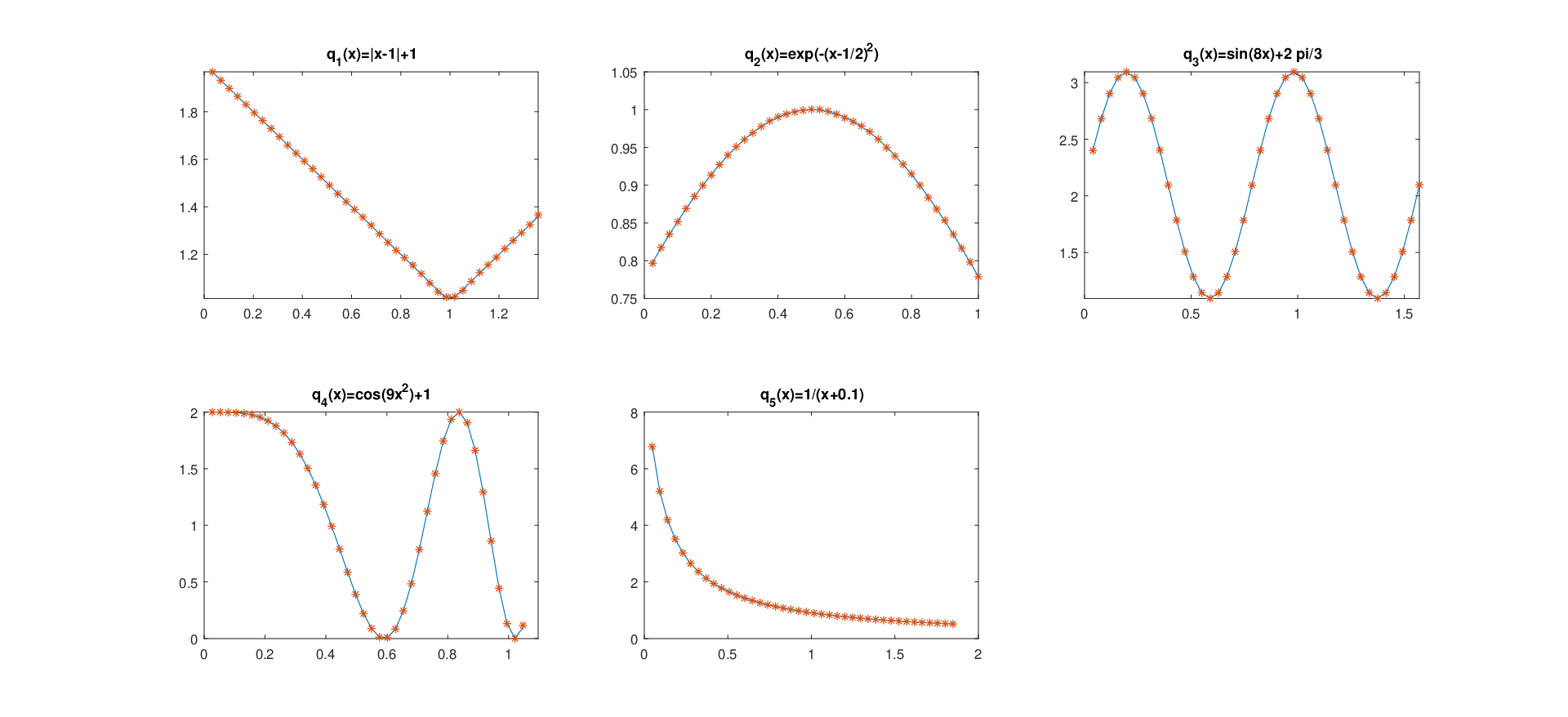
Example 1. Let us consider a star graph of five edges of lengths
| (6.1) |
The corresponding five components of the potential are defined as follows
| (6.2) |
| (6.3) |
We computed eigenvalues and corresponding norming constants as described in Section 4. In Table 1 some of the computed eigenvalues are presented.
Then to the computed spectral data we applied the method introduced in Section 5 for solving the inverse problem. The number of the coefficients in (5.5) and (5.8) was chosen . Our numerical experiments showed that even a more reduced number of the coefficients (say, five-six of them) gives already quite satisfactory (slightly less accurate) results. For the number from (5.15) was chosen the same value, , though this parameter, of course, may differ from .
In Fig. 1 we show the recovered potentials on the five edges. The absolute error of each recovered potential slightly grows at the endpoints of the interval attaining its maximum value in the second decimal digit (for at the origin), while in the interior points of the interval it remains two orders of magnitude smaller.
It is interesting to track how accurately the two spectra were computed on each edge. For example, Table 2 presents some of the “exact” Dirichlet-Dirichlet eigenvalues on computed with the aid of the Matslise package (first column), the approximate eigenvalues, computed as described in Subsection 5.1 by calculating zeros of and the absolute error of each presented eigenvalue. Notice that both the absolute and the relative errors remain small even for large indices.
| Table 2: Dirichlet-Dirichlet eigenvalues of | |||
Based on the computed Dirichlet-Dirichlet eigenvalues the parameter was computed for all , as explained in Subsection 5.1. In the case of the absolute error of the approximation was .
Next, using the quantum graph spectral eigendata and the computed the Dirichlet-Neumann eigenvalues for each potential component were computed. Table 3 presents the result of computation for . One can observe that while the accuracy is slightly worse than in the case of the Dirichlet-Dirichlet eigenvalues, it is still quite satisfactory and uniform.
| Table 3: Dirichlet-Neumann eigenvalues of | |||
In the considered example the worst accuracy was obtained for the component of the potential . Table 4 shows the accuracy of the Dirichlet-Dirichlet eigenvalues computed.
| Table 4: Dirichlet-Dirichlet eigenvalues of | |||
Based on this result, the approximation of the parameter resulted in the following value of the absolute error . Finally, some Dirichlet-Neumann eigenvalues for are presented in Table 5.
| Table 5: Dirichlet-Neumann eigenvalues of | |||
It is worth noting that the whole computation takes few seconds performed in Matlab 2017 on a Laptop equipped with a Core i7 Intel processor.
The method copes equally well with inverse spectral problems on star graphs with a larger number of edges, though to obtain similar accuracy in this case more spectral data are required.
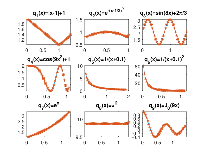
Example 2. Consider a nine edges quantum star graph with five edges and components of potential coinciding with those from the previous example and with the additional edges and the corresponding components of the potential
where stands for the Bessel function of the first kind of order zero. Fig. 2 presents the potential recovered from spectral data.
7 Conclusions
A new method for solving the inverse spectral problem on quantum star graphs is developed. The main role in the proposed approach is played by the coefficients of the Neumann series of Bessel functions expansion of solutions of the Sturm-Liouville equation. With their aid the given spectral data lead to separate two spectra Sturm-Liouville inverse problems on each edge. These two-spectra problems are solved by a direct method reducing each problem to a system of linear algebraic equations, and the crucial observation is that the potential is recovered from the first component of the solution vector.
The method is simple, direct and accurate. Its performance is illustrated by numerical examples. In subsequent works we plan to extend this method to other types of inverse spectral problems and to more general graphs.
Acknowledgements
Research was supported by CONACYT, Mexico via the project 284470 and partially performed at the Regional mathematical center of the Southern Federal University with the support of the Ministry of Science and Higher Education of Russia, agreement 075-02-2022-893. The research of Sergei Avdonin was supported in part by the National Science Foundation, grant DMS 1909869, and by Moscow Center for Fundamental and Applied Mathematics.
References
- [1] Abramovitz M. and Stegun I. A. (1972), Handbook of mathematical functions, New York: Dover.
- [2] Arioli M. and Benzi M. (2018), A finite element method for quantum graphs. IMA J. Numer. Anal., 38, no. 3, 1119–1163.
- [3] Avdonin S., Belinskiy B., and Matthews J. (2011), Inverse problem on the semi-axis: local approach, Tamkang Journal of Mathematics, 42, no. 3, 1–19.
- [4] Avdonin S. and Bell J. (2015), Determining physical parameters for a neuronal cable model defined on a tree graph, Journal of Inverse Problems and Imaging, 9, no. 3, 645-659.
- [5] Avdonin S. and Kravchenko V. V. (2022) Method for solving inverse spectral problems on quantum star graphs. Submitted.
- [6] Avdonin S. and Kurasov P. (2008), Inverse problems for quantum trees, Inverse Problems and Imaging, 2, no. 1, 1–21.
- [7] Avdonin S., Leugering G., and Mikhaylov V. (2010), On an inverse problem for tree-like networks of elastic strings, Zeit. Angew. Math. Mech., 90, no. 2, 136–150.
- [8] Belishev M. and Vakulenko A. (2006), Inverse problems on graphs: Recovering the tree of strings by the BC-method, J. Inv. Ill-Posed Problems, 14 , 29-46.
- [9] Berkolaiko G. and Kuchment P. (2013), Introduction to Quantum Graphs, AMS, Providence, R.I.
- [10] Brown B. M., Samko V. S., Knowles I. W., Marletta M. (2003), Inverse spectral problem for the Sturm–Liouville equation, Inverse Probl. 19 , 235–252.
- [11] Chadan Kh., Colton D., Päivärinta L., Rundell W. (1997), An introduction to inverse scattering and inverse spectral problems. SIAM, Philadelphia.
- [12] Kravchenko V. V. (2019), On a method for solving the inverse Sturm–Liouville problem, J. Inverse Ill-posed Probl. 27, 401–407.
- [13] Kravchenko V. V. (2020), Direct and inverse Sturm-Liouville problems: A method of solution, Birkhäuser, Cham.
- [14] Kravchenko V. V., Navarro L. J. and Torba S. M. (2017), Representation of solutions to the one-dimensional Schrödinger equation in terms of Neumann series of Bessel functions, Appl. Math. Comput. 314, 173–192.
- [15] Kravchenko V. V. and Torba S. M. (2015), Analytic approximation of transmutation operators and applications to highly accurate solution of spectral problems, Journal of Computational and Applied Mathematics 275, 1-26.
- [16] Kravchenko V. V. and Torba S. M. (2021), A direct method for solving inverse Sturm-Liouville problems, Inverse Probl. 37, 015015 (32pp).
- [17] Kurasov P. (2022) Quantum Graphs: Spectral Theory and Inverse Problems, Springer (to appear).
- [18] Kurasov P. and Nowaczyk M. (2005), Inverse spectral problem for quantum graphs, J. Phys. A., 38, 4901-4915.
- [19] Lagnese J.E., Leugering G., and Schmidt E.J.P.G. (1994), Modelling, Analysis and Control of Multi-Link Flexible Structures, Basel: Birkhäuser.
- [20] Levitan B. M. (1987), Inverse Sturm-Liouville problems, VSP, Zeist.
- [21] Mugnolo, D. (2014), Semigroup Methods for Evolution Equations on Networks, Understanding Complex Systems, Springer, Cham.
- [22] Shishkina E. L. and Sitnik S. M. (2020), Transmutations, singular and fractional differential equations with applications to mathematical physics, Elsevier, Amsterdam.
- [23] Savchuk A. M., Shkalikov A. A. (2005), Inverse problem for Sturm–Liouville operators with distribution potentials: reconstruction from two spectra, Russ. J. Math. Phys. 12, 507–514.
- [24] Yurko V. A. (2005), Inverse Sturm-Lioville operator on graphs, Inverse Problems, 21, 1075-1086.
- [25] Yurko V. A. (2007), Introduction to the theory of inverse spectral problems, Fizmatlit, Moscow, (in Russian).