跳到论文正文
W Papers独立论文阅读器 arXiv:2210.11925 论文正文 计算阅读时间 · 0%
引用这篇论文根据当前论文元数据生成,正式投稿前建议核对。


License: arXiv.org perpetual non-exclusive license
arXiv:2210.11925v3 [stat.ML] 28 Oct 2023

Unbiased constrained sampling with
Self-Concordant Barrier Hamiltonian Monte Carlo

Maxence Noble Thanks: Corresponding author. Contact at: maxence.noble-bourillot@polytechnique.edu Affiliation: CMAP, CNRS, École polytechnique, Affiliation: Institut Polytechnique de Paris, Affiliation: 91120 Palaiseau, France    Valentin De Bortoli Affiliation: Computer Science Department, Affiliation: ENS, CNRS, PSL University    Alain Oliviero Durmus Affiliation: CMAP, CNRS, École polytechnique, Affiliation: Institut Polytechnique de Paris, Affiliation: 91120 Palaiseau, France
Abstract

In this paper, we propose Barrier Hamiltonian Monte Carlo (BHMC), a version of the HMC algorithm which aims at sampling from a Gibbs distribution π\pi on a manifold 𝖬\mathsf{M}, endowed with a Hessian metric 𝔤\mathfrak{g} derived from a self-concordant barrier. Our method relies on Hamiltonian dynamics which comprises 𝔤\mathfrak{g}. Therefore, it incorporates the constraints defining 𝖬\mathsf{M} and is able to exploit its underlying geometry. However, the corresponding Hamiltonian dynamics is defined via non separable Ordinary Differential Equations (ODEs) in contrast to the Euclidean case. It implies unavoidable bias in existing generalization of HMC to Riemannian manifolds. In this paper, we propose a new filter step, called “involution checking step”, to address this problem. This step is implemented in two versions of BHMC, coined continuous BHMC (c-BHMC) and numerical BHMC (n-BHMC) respectively. Our main results establish that these two new algorithms generate reversible Markov chains with respect to π\pi and do not suffer from any bias in comparison to previous implementations. Our conclusions are supported by numerical experiments where we consider target distributions defined on polytopes.

1 Introduction

Markov Chain Monte Carlo (MCMC) methods is one of the primary algorithmic approaches to obtain approximate samples from a target distribution π\pi. They have been successively applied over these past decades in a large panel of practical settings, (Liu & Liu 2001). In particular, gradient-based MCMC methods have shown their efficiency and robustness in high-dimensional settings, and come nowadays with strong theoretical guarantees, (Dalalyan 2017; Durmus & Moulines 2017). However, they still struggle in facing the case where the target distribution is supported on a constrained subset 𝖬\mathsf{M} of ℝd\mathbb{R}^{d}, (Gelfand et al. 1992; Pakman & Paninski 2014; Lan & Shahbaba 2015). Yet, this problem appears in various fields; see e.g., (Morris 2002; Lewis et al. 2012; Thiele et al. 2013) with some important applications in computational statistics and biology.

Drawing samples from such distributions is indeed a challenging problem that has been intensively studied in the literature, (Dyer & Frieze 1991; Lovász & Simonovits 1993; Lovász & Kannan 1999; Lovász & Vempala 2007; Brubaker et al. 2012; Cousins & Vempala 2014; Pakman & Paninski 2014; Lan & Shahbaba 2015; Bubeck et al. 2015). In particular, some recent extensions of the popular Metropolis-Hastings (MH) algorithm to constrained spaces consist in designing proposals based on dynamics for which π\pi is invariant, (Zappa et al. 2018; Lelièvre et al. 2019; Lelièvre et al. 2022). In practice, the corresponding solutions are numerically integrated based on implicit and symplectic schemes, which however come with additional difficulties. As first observed by Zappa et al. 2018, an additional “involution checking step” in the usual MH filter is necessary to ensure that the resulting Markov kernel admits π\pi as a stationary distribution.

In this paper, we aim at generalizing this family of methods by taking into account the geometry of the constrained subspace, building on the Riemannian Manifold Hamiltonian Monte Carlo (RMHMC) algorithm introduced by Girolami & Calderhead 2011. Similarly to HMC, (Duane et al. 1987; Neal et al. 2011; Betancourt 2017), RMHMC aims to target a positive distribution π\pi on ℝd\mathbb{R}^{d} and relies on the integration of a canonical Hamiltonian equation. In contrast, RMHMC incorporates some geometrical information in the definition of the Hamiltonian via a Riemannian metric 𝔤\mathfrak{g} on ℝd\mathbb{R}^{d}. When considering applications of RMHMC to a convex, open and bounded subset 𝖬\mathsf{M}, a natural choice for this metric is the Hessian metric associated with a self-concordant barrier on 𝖬\mathsf{M}, (Nesterov & Nemirovskii 1994), as suggested by Kook et al. 2022a. We adopt here the same approach and now focus on a constrained subspace 𝖬\mathsf{M} which is assumed to be equipped with an appropriately designed “self-concordant” metric, (Nesterov & Nemirovskii 1994).

Given this setting, we propose the BHMC (Barrier HMC) algorithm. To the best of our knowledge, this is the first version of RMHMC incorporating an “involution checking step” to assess the issue of asymptotic bias arising from the use of implicit integration methods to solve the Hamiltonian dynamics. In this work, we focus on the numerical version of BHMC (n-BHMC), for which we provide a numerical implementation. We refer to Appendix D for an introduction to the ideal version of BHMC, called continuous BHMC (c-BHMC), where it is assumed that we have access to the continuous Hamiltonian dynamics but which cannot be computed in practice. For each algorithm, we rigorously prove that the associated Markov chain preserves π\pi.

The rest of the paper is organized as follows. In Section 2, we introduce our sampling framework and review some background on self-concordance and Riemannian geometry. In Section 3, we present n-BHMC, and derive theoretical results for this algorithm in Section 4. We review related works in Section 5 and provide numerical experiments for n-BHMC in Section 6.

Notation.

For any f∈C3​(ℝd,ℝ)f\in\mathrm{C}^{3}(\mathbb{R}^{d},\mathbb{R}), we denote by D​fDf (and D2​fD^{2}f) the Jacobian (resp. the Hessian) of ff. For any A∈ℝd×d\mathrm{A}\in\mathbb{R}^{d\times d} and any (x,y)∈ℝd×ℝd(x,y)\in\mathbb{R}^{d}\times\mathbb{R}^{d}, we denote by A:D3​f​(x)\mathrm{A}:D^{3}f(x) the vector (Tr⁡(A⊤​{D3​f​(x)}i))i∈[d]∈ℝd(\operatorname{Tr}(\mathrm{A}^{\top}\{D^{3}f(x)\}_{i}))_{i\in[d]}\in\mathbb{R}^{d}, and define D3​f​(x)​[x,y]D^{3}f(x)[x,y] as the vector x⊤​D3​f​(x)​y∈ℝdx^{\top}D^{3}f(x)y\in\mathbb{R}^{d}. For any positive-definite matrix A∈ℝd×d\mathrm{A}\in\mathbb{R}^{d\times d}, ⟨⋅,⋅⟩A\langle\cdot,\cdot\rangle_{\mathrm{A}} stands for the scalar product induced by A\mathrm{A} on ℝd\mathbb{R}^{d}, defined by ⟨x,y⟩A=⟨x,A​y⟩\langle x,y\rangle_{\mathrm{A}}=\langle x,\mathrm{A}y\rangle. The “momentum reversal” operator s:ℝd×ℝd→ℝd×ℝds:\ \mathbb{R}^{d}\times\mathbb{R}^{d}\to\mathbb{R}^{d}\times\mathbb{R}^{d} is defined for any (x,p)∈ℝd×ℝd(x,p)\in\mathbb{R}^{d}\times\mathbb{R}^{d} by s⁡(x,p)=(x,−p)s(x,p)=(x,-p). Let 𝖤,𝖥\mathsf{E},\mathsf{F} be two sets and h:𝖤→2𝖥h:\ \mathsf{E}\to 2^{\mathsf{F}}, where 2𝖥2^{\mathsf{F}} is the set of sets of 𝖥\mathsf{F}. We say that hh is a set-valued map. Note that any map g:𝖤→𝖥g:\mathsf{E}\to\mathsf{F} can be extended to a set-valued map by identifying, for any x∈𝖤x\in\mathsf{E}, g⁡(x)g(x) and {g⁡(x)}\{g(x)\}. Let f:𝖥→2𝖦f:\mathsf{F}\to 2^{\mathsf{G}}. We define f∘h:𝖤→2𝖦f\circ h:\ \mathsf{E}\to 2^{\mathsf{G}} for any x∈𝖤x\in\mathsf{E} by f∘h(x)=∪y∈h⁡(x)f(y)f\circ h(x)=\cup_{y\in h(x)}f(y), where by convention ∪∅=∅\cup_{\emptyset}=\emptyset. For any topological space 𝖷\mathsf{X}, we denote ℬ⁡(𝖷)\mathcal{B}(\mathsf{X}) its Borel sets. For any probability measure μ∈𝒫⁡(𝖷)\mu\in\mathscr{P}(\mathsf{X}) and measurable map φ:𝖷→𝖸\varphi:\mathsf{X}\to\mathsf{Y}, we denote φ#​μ∈𝒫⁡(𝖸)\varphi_{\#}\mu\in\mathscr{P}(\mathsf{Y}) the pushforward of μ\mu by φ\varphi. In general, we will equivalently denote by zz or (x,p)(x,p) a state of the Hamiltonian system.

2 Setting and Background

In this paper, we consider an open subset 𝖬⊂ℝd\mathsf{M}\subset\mathbb{R}^{d}, and we aim at sampling from a target distribution π\pi given for any x∈𝖬x\in\mathsf{M} by

d​π​(x)/d​x=exp⁡[−V⁡(x)]/Z,\displaystyle\mathrm{d}\pi(x)/\mathrm{d}x=\exp[-V(x)]/Z\;, (2)

where V∈C2​(𝖬,ℝ)V\in\mathrm{C}^{2}(\mathsf{M},\mathbb{R}) and Z=∫𝖬exp⁡[−V⁡(x)]​𝑑xZ=\textstyle{\int_{\mathsf{M}}\exp[-V(x)]\mathrm{d}x}. We view 𝖬\mathsf{M} as an embedded dd-dimensional submanifold of ℝd\mathbb{R}^{d}, equipped with a metric 𝔤\mathfrak{g}, satisfying the following assumptions.

A 1.

𝖬\mathsf{M} is an open convex bounded subset of ℝd\mathbb{R}^{d}.

A 2.

There exists ϕ\phi, a α\alpha-regular and ν\nu-self-concordant barrier on 𝖬\mathsf{M} such that 𝔤=D2​ϕ\mathfrak{g}=D^{2}\phi.

We provide in Section 2.1 basic Riemannian facts along with the definition of the Hamiltonian dynamics of RMHMC and introduce self-concordance and α\alpha-regularity in Section 2.2.

2.1 Riemannian Manifold Hamiltonian dynamics

Basics on Riemannian geometry.

Let 𝖬\mathsf{M} be a dd-dimensional smooth manifold, endowed with a metric 𝔤\mathfrak{g}. Denoting by d​x\mathrm{d}x a dual coframe, (Lee 2006, Lemma 3.2.), we recall that the Riemannian volume element corresponding to (𝖬,𝔤)(\mathsf{M},\mathfrak{g}) is given in local coordinates by

dvol𝖬​(x)=det(𝔤)​d​x.\displaystyle\mathrm{d}\mathrm{vol}_{\mathsf{M}}(x)=\sqrt{\det(\mathfrak{g})}\mathrm{d}x\;. (3)

We denote by Tx⋆​𝖬\mathrm{T}_{x}^{\star}\mathsf{M} the dual of the tangent space at x∈𝖬x\in\mathsf{M}, i.e., the cotangent space. For any x∈𝖬x\in\mathsf{M}, Tx⋆​𝖬\mathrm{T}_{x}^{\star}\mathsf{M} is a vector space naturally endowed with the scalar product ⟨⋅,⋅⟩𝔤​(x)−1\langle\cdot,\cdot\rangle_{\mathfrak{g}(x)^{-1}}, (Mok 1977). We recall that the cotangent bundle T⋆​𝖬\mathrm{T}^{\star}\mathsf{M} is defined by T⋆𝖬=⊔x∈𝖬{x}∪Tx⋆𝖬\mathrm{T}^{\star}\mathsf{M}=\sqcup_{x\in\mathsf{M}}\{x\}\cup\mathrm{T}_{x}^{\star}\mathsf{M}. This set is a 2​d2d-dimensional manifold endowed with a Riemannian metric 𝔤⋆\mathfrak{g}^{\star} given by Mok 1977, inherited from 𝔤\mathfrak{g}. With this metric, the volume form on T⋆​𝖬\mathrm{T}^{\star}\mathsf{M} does not depend on 𝔤\mathfrak{g} anymore, and satisfies for any (x,p)∈T⋆​𝖬(x,p)\in\mathrm{T}^{\star}\mathsf{M}

dvolT⋆​𝖬​(x,p)=d​x​d​p,\textstyle{\mathrm{d}\mathrm{vol}_{\mathrm{T}^{\star}\mathsf{M}}(x,p)=\mathrm{d}x\mathrm{d}p\;}\;, (4)

where d​x​d​p\mathrm{d}x\mathrm{d}p is a dual coframe for T⋆​𝖬\mathrm{T}^{\star}\mathsf{M}.

Therefore, under 1, identifying T⋆​𝖬\mathrm{T}^{\star}\mathsf{M} with 𝖬×ℝd\mathsf{M}\times\mathbb{R}^{d}, the volume form on T⋆​𝖬\mathrm{T}^{\star}\mathsf{M} induced by 𝔤⋆\mathfrak{g}^{\star} is the Lebesgue measure of ℝd×ℝd\mathbb{R}^{d}\times\mathbb{R}^{d} restricted to T⋆​𝖬\mathrm{T}^{\star}\mathsf{M}. Despite adopting at first a Riemannian perspective on 𝖬\mathsf{M}, we actually recover the Euclidean setting on T⋆​𝖬\mathrm{T}^{\star}\mathsf{M}, which motivates us to consider T⋆​𝖬\mathrm{T}^{\star}\mathsf{M} as our sampling space. We refer to Appendix B for details on the cotangent bundle and its metric 𝔤⋆\mathfrak{g}^{\star}.

Hamiltonian dynamics.

Note that with the previously introduced notation, π\pi can be expressed as

d​π/dvol𝖬​(x)=exp⁡[−V⁡(x)−12​log⁡(det(𝔤⁡(x)))]/Z.\displaystyle\mathrm{d}\pi/\mathrm{d}\mathrm{vol}_{\mathsf{M}}(x)=\exp[-V(x)-\tfrac{1}{2}\log(\det(\mathfrak{g}(x)))]/Z\;. (5)

This motivates the introduction of the following Hamiltonian on T⋆​𝖬\mathrm{T}^{\star}\mathsf{M}

H⁡(x,p)=V⁡(x)+12​log⁡(det⁡𝔤⁡(x))+12​‖p‖𝔤​(x)−12.H(x,p)=V(x)+\tfrac{1}{2}\log\left(\operatorname{det}\mathfrak{g}(x)\right)+\tfrac{1}{2}\|p\|_{\mathfrak{g}(x)^{-1}}^{2}\;. (6)

In this definition, we notably take into account the scalar product ⟨⋅,⋅⟩𝔤​(x)−1\langle\cdot,\cdot\rangle_{\mathfrak{g}(x)^{-1}} on Tx⋆​𝖬\mathrm{T}^{\star}_{x}\mathsf{M}. Finally, we consider the joint distribution π¯\bar{\pi} on T⋆​𝖬\mathrm{T}^{\star}\mathsf{M}

d​π¯​(x,p)=(1/Z¯)​exp⁡[−H⁡(x,p)]​dvolT⋆​𝖬​(x,p),\mathrm{d}\bar{\pi}(x,p)=(1/\bar{Z})\exp[-H(x,p)]\mathrm{d}\mathrm{vol}_{\mathrm{T}^{\star}\mathsf{M}}(x,p)\;, (7)

where Z¯=∫T⋆​𝖬exp⁡[−H⁡(x,p)]​dvolT⋆​𝖬​(x,p)\bar{Z}=\int_{\mathrm{T}^{\star}\mathsf{M}}\exp[-H(x,p)]\mathrm{d}\mathrm{vol}_{\mathrm{T}^{\star}\mathsf{M}}(x,p), for which the first marginal is π\pi. Indeed, for any φ∈C⁡(𝖬,ℝ)\varphi\in\mathrm{C}(\mathsf{M},\mathbb{R}), we have

∫T⋆​𝖬φ⁡(x)​𝑑π¯​(x,p)\displaystyle\textstyle{\int_{\mathrm{T}^{\star}\mathsf{M}}\varphi(x)\mathrm{d}\bar{\pi}(x,p)} =∫T⋆​𝖬φ⁡(x)​𝑑π​(x)​Nx​(p,0,Id)​𝑑p=∫𝖬φ⁡(x)​𝑑π​(x),\displaystyle\textstyle{=\int_{\mathrm{T}^{\star}\mathsf{M}}\varphi(x)\mathrm{d}\pi(x)\mathrm{N}_{x}(p;0,\mathrm{Id})\mathrm{d}p=\int_{\mathsf{M}}\varphi(x)\mathrm{d}\pi(x)\;,} (8)

where we denote by Nx​(0,Id)\mathrm{N}_{x}(0,\mathrm{I}_{d}) the centered standard Gaussian distribution w.r.t. ∥⋅∥𝔤​(x)−1\|\cdot\|_{\mathfrak{g}(x)^{-1}}. The Hamiltonian dynamics for HH is given by the coupled Ordinary Differential Equations (ODEs)

x˙=∂pH(x,p),p˙=−∂xH(x,p),\dot{x}=\partial_{p}H(x,p)\;,\qquad\dot{p}=-\partial_{x}H(x,p)\;, (9)

where the derivatives of HH can be computed explicitly as

∂pH⁡(x,p)=𝔤​(x)−1​p,∂xH⁡(x,p)=−12​D​𝔤​(x)​[𝔤​(x)−1​p,𝔤​(x)−1​p]+L⁡(x),\displaystyle\partial_{p}H(x,p)=\mathfrak{g}(x)^{-1}p\;,\qquad\partial_{x}H(x,p)=-\tfrac{1}{2}D\mathfrak{g}(x)[\mathfrak{g}(x)^{-1}p,\mathfrak{g}(x)^{-1}p]+L(x)\;, (10)

where L⁡(x)=∇V​(x)+12​𝔤​(x)−1:D​𝔤​(x)L(x)=\nabla V(x)+\tfrac{1}{2}\mathfrak{g}(x)^{-1}:D\mathfrak{g}(x).

2.2 Self-concordance and regularity

Until now, we have considered an arbitrary Riemannian metric 𝔤\mathfrak{g}. In the rest of this work, we focus on metrics given by Hessian of self-concordant barriers.

Self-concordance.

We first introduce self-concordant barriers, a family of smooth convex functions which are well-suited for minimization by the Newton method.

Definition 1 (Nesterov & Nemirovskii 1994).

Let 𝖴\mathsf{U} be a non-empty open convex domain in ℝd\mathbb{R}^{d}. A function ϕ:𝖴→ℝ\phi:\mathsf{U}\rightarrow\mathbb{R} is said to be a ν\nu-self-concordant barrier (with ν≥1\nu\geq 1) on 𝖴\mathsf{U} if it satisfies:

  1. (a)

    ϕ∈C3​(𝖴,ℝ)\phi\in\mathrm{C}^{3}(\mathsf{U},\mathbb{R}) and ϕ\phi is convex,

  2. (b)

    ϕ⁡(x)→+∞\phi(x)\xrightarrow{}+\infty as x→∂𝖴x\rightarrow\partial\mathsf{U},

  3. (c)

    |D3​ϕ​(x)​[h,h,h]|≤2​‖h‖𝔤⁡(x)3|D^{3}\phi(x)[h,h,h]|\leq 2\|h\|_{\mathfrak{g}(x)}^{3}, for any x∈𝖬x\in\mathsf{M}, h∈ℝdh\in\mathbb{R}^{d},

  4. (d)

    |D​ϕ​(x)​[h]|2≤ν​‖h‖𝔤⁡(x)2|D\phi(x)[h]|^{2}\leq\nu\|h\|_{\mathfrak{g}(x)}^{2}, for any x∈𝖬x\in\mathsf{M}, h∈ℝdh\in\mathbb{R}^{d},

where 𝔤⁡(x)=D2​ϕ​(x)\mathfrak{g}(x)=D^{2}\phi(x).

Balls for ‖⋅‖𝔤⁡(x)\left\|\cdot\right\|_{\mathfrak{g}(x)}, called Dikin ellipsoids, are key for the study of self-concordance, see Appendix C.

Regularity.

The property of α\alpha-regularity for some α≥1\alpha\geq 1 is shared by many self-concordant barriers, including logarithmic and quadratic programming barriers. It ensures stability for interior point polynomial-time methods. Definition and properties of α\alpha-regularity are recalled in Appendix C.

Refer to caption
Figure 1: A polytope 𝖬⊂ℝ2\mathsf{M}\subset\mathbb{R}^{2} with three Dikin ellipsoids {y∈ℝd:y⊤​𝔤​(x)​y<1}\{y\in\mathbb{R}^{d}\,:\;y^{\top}\mathfrak{g}(x)y<1\} derived from its logarithmic barrier.

Example of the polytope.

Let us assume that 𝖬\mathsf{M} is the polytope 𝖬={x:A​x<b}\mathsf{M}=\{x:\mathrm{A}x<b\}, where A∈ℝm×d\mathrm{A}\in\mathbb{R}^{m\times d} and b∈ℝmb\in\mathbb{R}^{m}. We endow it with the Riemannian metric 𝔤⁡(x)=D2​ϕ​(x)\mathfrak{g}(x)=D^{2}\phi(x) where ϕ:𝖬→ℝ\phi:\mathsf{M}\rightarrow\mathbb{R} is the logarithmic barrier given for any x∈𝖬x\in\mathsf{M} by ϕ(x)=−∑i=1mlog(bi−Ai⊤x)\phi(x)=-\sum_{i=1}^{m}\log\left(b_{i}-\mathrm{A}_{i}^{\top}x\right). The barrier ϕ\phi is both a mm-self-concordant barrier and a 22-regular function, (Nesterov & Nemirovski 1998, page 3). Moreover, we have for any x∈𝖬x\in\mathsf{M}, 𝔤⁡(x)=A⊤​S​(x)−2​A\mathfrak{g}(x)=\mathrm{A}^{\top}S(x)^{-2}\mathrm{A}, where S⁡(x)=Diag​(bi−Ai⊤​x)i∈[m]S(x)=\text{Diag}\left(b_{i}-\mathrm{A}_{i}^{\top}x\right)_{i\in[m]}. We provide in Figure 1 an illustration of this barrier.

3 The n-BHMC algorithm

In practice, it is not possible to exactly compute the Riemannian Hamiltonian dynamics (9). We thus introduce a numerical version of BHMC (n-BHMC), in which we replace the continuous ODE integration by a symplectic numerical scheme. We first define the Hamiltonian integrators used in n-BHMC in Section 3.1 and provide details on the different steps of our algorithm in Section 3.2.

3.1 Hamiltonian integrators of n-BHMC

In the same spirit as Shahbaba et al. 2014, we first rewrite the Hamiltonian HH given in (6) as H=H1+H2H=H_{1}+H_{2}, where we highlight the non separable aspect of HH in H2H_{2}, i.e., for any (x,p)∈T⋆​𝖬(x,p)\in\mathrm{T}^{\star}\mathsf{M}

H1​(x,p)=V⁡(x)+12​log⁡(det⁡𝔤⁡(x)),H2​(x,p)=12​‖p‖𝔤​(x)−12.\textstyle{H_{1}(x,p)=V(x)+\tfrac{1}{2}\log(\operatorname{det}\mathfrak{g}(x))\;,\quad H_{2}(x,p)=\tfrac{1}{2}\|p\|^{2}_{\mathfrak{g}(x)^{-1}}\;.} (11)

Therefore, we have

∂xH1​(x,p)\displaystyle\partial_{x}H_{1}(x,p) =∇V​(x)+12​𝔤​(x)−1:D​𝔤​(x),\displaystyle=\nabla V(x)+\tfrac{1}{2}\mathfrak{g}(x)^{-1}:D\mathfrak{g}(x)\;, ∂pH1​(x,p)=0,\displaystyle\partial_{p}H_{1}(x,p)=0\;, (12)
∂xH2​(x,p)\displaystyle\partial_{x}H_{2}(x,p) =−12​D​𝔤​(x)​[𝔤​(x)−1​p,𝔤​(x)−1​p],\displaystyle=-\tfrac{1}{2}D\mathfrak{g}(x)[\mathfrak{g}(x)^{-1}p,\mathfrak{g}(x)^{-1}p]\;, ∂pH2​(x,p)=𝔤​(x)−1​p.\displaystyle\partial_{p}H_{2}(x,p)=\mathfrak{g}(x)^{-1}p\;. (13)

Leveraging the separable structure of H1H_{1}, we now define an implicit scheme to discretize the Hamiltonian dynamics (9) by splitting it into the Hamiltonian dynamics (12) and (13). In the rest of this section, we consider some step-size h∈ℝh\in\mathbb{R}.

Explicit integrator of H1H_{1}.

We first approximate the dynamics (12) on a step-size h/2h/2 using a first-order Euler method (Hairer et al. 2006, Theorem VI.3.3.). Since H1H_{1} is separable, this integrator simply reduces to the map Sh/2:T⋆​𝖬→T⋆​𝖬\mathrm{S}_{h/2}:\mathrm{T}^{\star}\mathsf{M}\to\mathrm{T}^{\star}\mathsf{M} defined by

Sh/2​(x,p)=(x,p−h2​∂xH1​(x,p)).\textstyle{\mathrm{S}_{h/2}(x,p)=(x,p-\tfrac{h}{2}\partial_{x}H_{1}(x,p))\;.} (14)

We have: (i) Sh/2​(T⋆​𝖬)⊂T⋆​𝖬\mathrm{S}_{h/2}(\mathrm{T}^{\star}\mathsf{M})\subset\mathrm{T}^{\star}\mathsf{M}, (ii) Sh/2\mathrm{S}_{h/2} is symplectic (we refer to Appendix F for more details on symplecticity), (iii) S−h/2∘Sh/2=Id\mathrm{S}_{-h/2}\circ\mathrm{S}_{h/2}=\text{Id} and (iv) S−h/2=s∘Sh/2∘s\mathrm{S}_{-h/2}=s\circ\mathrm{S}_{h/2}\circ s. Note that s∘Sh/2s\circ\mathrm{S}_{h/2} is an involution on T⋆​𝖬\mathrm{T}^{\star}\mathsf{M}, which inherits from properties (i) and (ii) of Sh/2\mathrm{S}_{h/2}.

Implicit integrator of H2H_{2}.

Since H2H_{2} is not separable, a common discretization scheme such as the Euler method is not symplectic anymore, which requires to use an implicit method instead. We thus approximate these dynamics on a step-size hh with a symplectic second-order integrator denoted by Gh\mathrm{G}_{h}. For theoretical purposes, we focus on the Störmer-Verlet scheme, (Hairer et al. 2006, Theorem VI.3.4.), also known as the generalized Leapfrog integrator, which is widely used in geometric integration, (Girolami & Calderhead 2011; Betancourt 2013; Cobb et al. 2019; Brofos & Lederman 2021a). We refer to Appendix F for a discussion on other numerical schemes. For any z(0)∈T⋆​𝖬z^{(0)}\in\mathrm{T}^{\star}\mathsf{M}, Gh​(z(0))⊂T⋆​𝖬\mathrm{G}_{h}(z^{(0)})\subset\mathrm{T}^{\star}\mathsf{M} consists of points z(1)=(x(1),p(1))z^{(1)}=(x^{(1)},p^{(1)}) which are solution of

p(1/2)\displaystyle p^{(1/2)} =p(0)−h2​∂xH2​(x(0),p(1/2)),\displaystyle=p^{(0)}-\tfrac{h}{2}\partial_{x}H_{2}(x^{(0)},p^{(1/2)})\;, (15)
x(1)\displaystyle x^{(1)} =x(0)+h2​[∂pH2​(x(0),p(1/2))+∂pH2​(x(1),p(1/2))],\displaystyle=x^{(0)}+\tfrac{h}{2}[\partial_{p}H_{2}(x^{(0)},p^{(1/2)})+\partial_{p}H_{2}(x^{(1)},p^{(1/2)})]\;, (16)
p(1)\displaystyle p^{(1)} =p(1/2)−h2​∂xH2​(x(1),p(1/2)).\displaystyle=p^{(1/2)}-\tfrac{h}{2}\partial_{x}H_{2}(x^{(1)},p^{(1/2)})\;. (17)

As defined, there is no guarantee that (17) admits a (unique) solution. As a matter of fact, the integrator Gh\mathrm{G}_{h} can be seen as a set-valued map. Moreover, it is easy to check that: (i) Gh​(T⋆​𝖬)⊂2T⋆​𝖬\mathrm{G}_{h}(\mathrm{T}^{\star}\mathsf{M})\subset 2^{\mathrm{T}^{\star}\mathsf{M}}, (ii) G−h=s∘Gh∘s\mathrm{G}_{-h}=s\circ\mathrm{G}_{h}\circ s, since ∂pH2(s(z))=−∂pH2(z)\partial_{p}H_{2}(s(z))=-\partial_{p}H_{2}(z) and ∂xH2​(s⁡(z))=∂xH2​(z)\partial_{x}H_{2}(s(z))=\partial_{x}H_{2}(z), and (iii) if |Gh​(z)|>0|\mathrm{G}_{h}(z)|>0 then z∈(G−h∘Gh)​(z)z\in(\mathrm{G}_{-h}\circ\mathrm{G}_{h})(z).

Implicit integrator of HH.

Relying on the integrators Sh/2\mathrm{S}_{h/2} and Gh\mathrm{G}_{h} previously defined, we now explain how we approximate the Hamiltonian dynamics (9) on a step-size hh. We first define the set-valued maps Fh:T⋆​𝖬→2T⋆​𝖬\mathrm{F}_{h}:\mathrm{T}^{\star}\mathsf{M}\rightarrow 2^{\mathrm{T}^{\star}\mathsf{M}} and Rh:T⋆​𝖬→2T⋆​𝖬\mathrm{R}_{h}:\mathrm{T}^{\star}\mathsf{M}\rightarrow 2^{\mathrm{T}^{\star}\mathsf{M}} by

Fh=Gh∘s,Rh=(s∘Sh/2)∘Fh∘(s∘Sh/2).\textstyle{\mathrm{F}_{h}=\mathrm{G}_{h}\circ s\;,\quad\mathrm{R}_{h}=(s\circ\mathrm{S}_{h/2})\circ\mathrm{F}_{h}\circ(s\circ\mathrm{S}_{h/2})\;.} (18)

Using properties (ii) and (iii) of Gh\mathrm{G}_{h}, we have for any z∈T⋆​𝖬z\in\mathrm{T}^{\star}\mathsf{M} such that |Fh​(z)|>0|\mathrm{F}_{h}(z)|>0, z∈(Fh∘Fh)​(z)z\in(\mathrm{F}_{h}\circ\mathrm{F}_{h})(z), and for any z′∈T⋆​𝖬z^{\prime}\in\mathrm{T}^{\star}\mathsf{M} such that |(Fh∘s∘Sh/2)​(z′)|>0|(\mathrm{F}_{h}\circ s\circ\mathrm{S}_{h/2})(z^{\prime})|>0, we have z′∈(Rh∘Rh)​(z′)z^{\prime}\in(\mathrm{R}_{h}\circ\mathrm{R}_{h})(z^{\prime}). Thus, Fh\mathrm{F}_{h} and Rh\mathrm{R}_{h} are involutive in the sense of set-valued maps. Note also that s∘Rh=Sh/2∘Gh∘Sh/2s\circ\mathrm{R}_{h}=\mathrm{S}_{h/2}\circ\mathrm{G}_{h}\circ\mathrm{S}_{h/2} boils down to the Strang splitting (Strang 1968) of the dynamics (9) and thus, is a symplectic scheme approximating the dynamics of Hamiltonian HH on a step-size hh.

Numerical integrators.

In practice, we do not have access to Fh\mathrm{F}_{h} but approximate it with a numerical map Φh\Phi_{h}. For clarity’s sake, we denote by domΦh⊂T⋆​𝖬\mathrm{dom}_{\Phi_{h}}\subset\mathrm{T}^{\star}\mathsf{M} the domain of this integrator with Φh​(domΦh)⊂T⋆​𝖬\Phi_{h}(\mathrm{dom}_{\Phi_{h}})\subset\mathrm{T}^{\star}\mathsf{M}. In practice, domΦh\mathrm{dom}_{\Phi_{h}} corresponds to the set of points for which the numerical integration of Fh\mathrm{F}_{h} outputs a solution. We also approximate Rh\mathrm{R}_{h} with the numerical map RhΦ:(s∘Sh/2)​(domΦh)⊂T⋆​𝖬→T⋆​𝖬\mathrm{R}_{h}^{\Phi}:(s\circ\mathrm{S}_{h/2})(\mathrm{dom}_{\Phi_{h}})\subset\mathrm{T}^{\star}\mathsf{M}\rightarrow\mathrm{T}^{\star}\mathsf{M}

RhΦ=(s∘Sh/2)∘Φh∘(s∘Sh/2).\mathrm{R}_{h}^{\Phi}=(s\circ\mathrm{S}_{h/2})\circ\Phi_{h}\circ(s\circ\mathrm{S}_{h/2})\;. (19)

Similarly to s∘Rhs\circ\mathrm{R}_{h}, s∘RhΦs\circ\mathrm{R}_{h}^{\Phi}11 1 Note that s∘RhΦs\circ\mathrm{R}_{h}^{\Phi} is a function and not a set-valued map. approximates the dynamics of Hamiltonian HH on a step-size hh. In our experiments, we design Φh\Phi_{h} using a fixed-point solver with a given number of iterations following Brofos & Lederman 2021a; Brofos & Lederman 2021b. We refer to Appendix K for details on computations of Φh\Phi_{h}.

3.2 Steps of the algorithm

For any z=(x,p)∈T⋆​𝖬z=(x,p)\in\mathrm{T}^{\star}\mathsf{M}, we define on T⋆​𝖬\mathrm{T}^{\star}\mathsf{M} the norm ∥⋅∥z\|\cdot\|_{z} by

‖(x′,p′)‖z=‖x′‖𝔤⁡(x)+‖p′‖𝔤​(x)−1,∀(x′,p′)∈T⋆​𝖬,\displaystyle\|(x^{\prime},p^{\prime})\|_{z}=\|x^{\prime}\|_{\mathfrak{g}(x)}+\|p^{\prime}\|_{\mathfrak{g}(x)^{-1}}\;,\quad\forall(x^{\prime},p^{\prime})\in\mathrm{T}^{\star}\mathsf{M}\;, (20)

where ∥⋅∥𝔤​(x)−1\|\cdot\|_{\mathfrak{g}(x)^{-1}} is the canonical norm on Tx⋆​𝖬\mathrm{T}_{x}^{\star}\mathsf{M} induced by the Riemannian metric 𝔤\mathfrak{g} (see Section 2.1) and ∥⋅∥𝔤⁡(x)\|\cdot\|_{\mathfrak{g}(x)} is the common norm used on 𝖬\mathsf{M} to study properties of self-concordance (see Section 2.2). As defined, this norm will be crucial to correct the bias of the numerical integration in n-BHMC, presented in Algorithm 1, for which we are now ready to detail the steps.

Steps 1 and 5: applying a momentum update.

Assume that the current state at stage n≥1n\geq 1 is (Xn−1,Pn−1)∈T⋆​𝖬(X_{n-1},P_{n-1})\in\mathrm{T}^{\star}\mathsf{M}. Then, the momentum is first partially refreshed such that P~n←1−β​Pn−1+β​Gn\tilde{P}_{n}\leftarrow\sqrt{1-\beta}P_{n-1}+\sqrt{\beta}G_{n}, where Gn∼Nx​(0,Id)G_{n}\sim\mathrm{N}_{x}(0,\mathrm{I}_{d}) is independent from Pn−1P_{n-1}. This update is applied both at the beginning and the end of the iteration, similarly to Lelièvre et al. 2022.

Step 2: solving a discretized version of ODE (9).

Starting from (Xn′,Pn′)=(Xn−1,P~n)(X^{\prime}_{n},P^{\prime}_{n})=(X_{n-1},\tilde{P}_{n}), we now approximate the dynamics of HH on a step-size hh with the integrators presented in Section 3.1, while ensuring that the proposal state belongs to T⋆​𝖬\mathrm{T}^{\star}\mathsf{M}. We proceed as follows:

  1. 1.

    We first run the explicit integrator Sh/2\mathrm{S}_{h/2} and compute Zn(0)=(s∘Sh/2)​(Xn−1,P~n)Z_{n}^{(0)}=(s\circ\mathrm{S}_{h/2})(X_{n-1},\tilde{P}_{n}).

  2. 2.

    If Zn(0)∉domΦhZ_{n}^{(0)}\notin\mathrm{dom}_{\Phi_{h}}, then (Xn′,Pn′)(X^{\prime}_{n},P^{\prime}_{n}) is not updated and we directly go to Step 3. Otherwise, we define Zn(1)=Φh​(Zn(0))Z_{n}^{(1)}=\Phi_{h}(Z_{n}^{(0)}). To ensure the reversibility of this step, we then perform an “involution checking step”, (Zappa et al. 2018; Lelièvre et al. 2019), highlighted in yellow in Algorithm 1, i.e., we verify (a) Zn(1)∈domΦhZ_{n}^{(1)}\in\mathrm{dom}_{\Phi_{h}} and (b) Zn(0)=Φh​(Zn(1))Z_{n}^{(0)}=\Phi_{h}(Z_{n}^{(1)}). In practice, we replace condition (b) by combining an explicit tolerance threshold η\eta with the norm defined in (20) and accept the proposal if

    ‖Zn(0)−Φh​(Zn(1))‖Zn(0)+‖Zn(0)−Φh​(Zn(1))‖Φh​(Zn(1))≤η.\displaystyle\|Z_{n}^{(0)}-\Phi_{h}(Z_{n}^{(1)})\|_{Z_{n}^{(0)}}+\|Z_{n}^{(0)}-\Phi_{h}(Z_{n}^{(1)})\|_{\Phi_{h}(Z_{n}^{(1)})}\leq\eta\;. (21)

    We discuss the choice of this norm to perform the “involution checking step” in Appendix K. If both of these conditions are satisfied, we finally set (Xn′,Pn′)=(s∘Sh/2)​(Zn(1))(X_{n}^{\prime},P_{n}^{\prime})=(s\circ\mathrm{S}_{h/2})(Z_{n}^{(1)}), to ensure the reversibility of the update of (Xn′,Pn′)(X_{n}^{\prime},P_{n}^{\prime}). Otherwise, (Xn′,Pn′)(X_{n}^{\prime},P_{n}^{\prime}) is not updated and we go to Step 3.

Input: (X0,P0)∈T⋆​𝖬(X_{0},P_{0})\in\mathrm{T}^{\star}\mathsf{M}, β∈(0,1]\beta\in(0,1], N∈ℕN\in\mathbb{N}, h>0h>0, η>0\eta>0, Φh\Phi_{h} with domain domΦh\mathrm{dom}_{\Phi_{h}}
Output: (Xn,Pn)n∈[N](X_{n},P_{n})_{n\in[N]}
for n=1,…,Nn=1,...,N do 1
Step 1: Gn∼Nx​(0,Id),P~n←1−β​Pn−1+β​GnG_{n}\sim\mathrm{N}_{x}(0,\mathrm{I}_{d}),\tilde{P}_{n}\leftarrow\sqrt{1-\beta}P_{n-1}+\sqrt{\beta}G_{n}
Step 2: solving a discretized version of ODE (9)
Xn′,Pn′←Xn−1,P~nX^{\prime}_{n},P^{\prime}_{n}\leftarrow X_{n-1},\tilde{P}_{n};  Xn(0),Pn(0)←(s∘Sh/2)​(Xn,P~n)X_{n}^{(0)},P_{n}^{(0)}\leftarrow(s\circ\mathrm{S}_{h/2})(X_{n},\tilde{P}_{n})
if Zn(0)=(Xn(0),Pn(0))∈domΦhZ_{n}^{(0)}=(X_{n}^{(0)},P_{n}^{(0)})\in\mathrm{dom}_{\Phi_{h}} then
2
      Zn(1)=Φh​(Zn(0))Z_{n}^{(1)}=\Phi_{h}(Z_{n}^{(0)})
err0=‖Zn(0)−Φh​(Zn(1))‖Zn(0),err1=‖Zn(0)−Φh​(Zn(1))‖Φh​(Zn(1))\mathrm{err}_{0}=\|Z_{n}^{(0)}-\Phi_{h}(Z_{n}^{(1)})\|_{Z_{n}^{(0)}},\hskip 8.50012pt\mathrm{err}_{1}=\|Z_{n}^{(0)}-\Phi_{h}(Z_{n}^{(1)})\|_{\Phi_{h}(Z_{n}^{(1)})} (if defined)
if Zn(1)∈domΦh​ & ​err0+err1≤ηZ_{n}^{(1)}\in\mathrm{dom}_{\Phi_{h}}\textbf{ \& }\mathrm{err}_{0}+\mathrm{err}_{1}\leq\eta then Xn′,Pn′←(s∘Sh/2)​(Zn(1))X_{n}^{\prime},P_{n}^{\prime}\leftarrow(s\circ\mathrm{S}_{h/2})(Z_{n}^{(1)}) 3
           end if 4
     Step 3: An←min⁡(1,exp⁡[−H⁡(Xn′,Pn′)+H⁡(Xn−1,P~n)])A_{n}\leftarrow\min(1,\exp[-H(X_{n}^{\prime},P_{n}^{\prime})+H(X_{n-1},\tilde{P}_{n})]);  Un∼U⁡[0,1]U_{n}\sim U[0,1]
if Un≤AnU_{n}\leq A_{n} then X¯n,P¯n←Xn′,Pn′\bar{X}_{n},\bar{P}_{n}\leftarrow X_{n}^{\prime},P_{n}^{\prime} 5
      else X¯n,P¯n←Xn−1,P~n\bar{X}_{n},\bar{P}_{n}\leftarrow X_{n-1},\tilde{P}_{n} 6
      Step 4: Xn,P^n←s⁡(X¯n,P¯n)X_{n},\hat{P}_{n}\leftarrow s(\bar{X}_{n},\bar{P}_{n})
Step 5: Gn′∼Nx​(0,Id),Pn←1−β​P^n+β​Gn′G_{n}^{\prime}\sim\mathrm{N}_{x}(0,\mathrm{I}_{d}),P_{n}\leftarrow\sqrt{1-\beta}\hat{P}_{n}+\sqrt{\beta}G_{n}^{\prime} end for 7
Algorithm 1 n-BHMC with Momentum Refresh

Step 3: computing the acceptance filter.

We denote by a(x′,p′|x,p)a(x^{\prime},p^{\prime}|x,p) the acceptance probability to move from (x,p)∈T⋆​𝖬(x,p)\in\mathrm{T}^{\star}\mathsf{M} to (x′,p′)∈T⋆​𝖬(x^{\prime},p^{\prime})\in\mathrm{T}^{\star}\mathsf{M}, which is given by

a(x′,p′|x,p)=1∧exp[−H(x′,p′)+H(x,p)].a(x^{\prime},p^{\prime}|x,p)=1\wedge\exp[-H(x^{\prime},p^{\prime})+H(x,p)]\;. (22)

After Step 2, we perform a simple MH filter by accepting the proposal with probability An=a(Xn′,Pn′|Xn−1,P~n)A_{n}=a(X_{n}^{\prime},P_{n}^{\prime}|X_{n-1},\tilde{P}_{n}) similarly to a classical HMC algorithm.

Step 4: applying momentum reversal.

To ensure a move along the dynamics of HH with step-size hh, we reverse the momentum after the acceptance step. Indeed, if the acceptance filter is successful, then (Xn,P^n)=(s∘RhΦ)​(Xn−1,P~n−1)(X_{n},\hat{P}_{n})=(s\circ\mathrm{R}_{h}^{\Phi})(X_{n-1},\tilde{P}_{n-1}) approximates the Hamiltonian dynamics (9) on a step-size hh starting at (Xn−1,P~n−1)(X_{n-1},\tilde{P}_{n-1}), as seen in Section 3.1. Otherwise, (Xn,P^n)=(Xn−1,−P~n−1)(X_{n},\hat{P}_{n})=(X_{n-1},-\tilde{P}_{n-1}).

3.3 About the usefulness of the “involution checking step”

In their paper, Kook et al. 2022a also incorporate self-concordance into RMHMC to sample from distributions supported on polytopes. To integrate the Hamiltonian dynamics, they propose to use a numerical version of the Implicit Midpoint integrator (Hairer et al. 2006, Theorem VI.3.5.), which shares the same theoretical properties as the Störmer-Verlet scheme. This results in CRHMC (Kook et al. 2022a, Algorithm 3), whose main difference compared to n-BHMC is the lack of the “involution checking step” (Line 8 in Algorithm 1). Crucially, Kook et al. 2022a assume that their implicit integrator admits a unique solution given any starting point and any step-size hh, which is then approximated by their numerical scheme. However, this statement may not be true in the self-concordant setting, as we explain below with a simple example. This explains why we always refer to the implicit integrator as a set-valued map. In their setting, the numerical integrator is not guaranteed to be involutive, which results in an asymptotic bias that the MH filter cannot solve.

In our paper, we do not make such an assumption on the Störmer-Verlet integrator, and consider a numerical solver which outputs one approximate solution to this implicit scheme. By doing so, our analysis is meant to be as close as possible to the practical implementation of RMHMC. Then, the “involution checking step” is critical to make the numerical integrator locally involutive, which enables us to derive rigorous reversibility results, see Theorem 3, and to solve the issue of asymptotic bias caused by implicit integration, see Section 6. We refer to Appendix J for a detailed comparison between n-BHMC and CRHMC. We now present a simple setting where the assumption made by Kook et al. 2022a does not hold in the case of the Störmer-Verlet integrator, which is defined in (17).

Consider the 1-dimensional setting 𝖬=(−∞,0)\mathsf{M}=(-\infty,0) with 𝔤:x↦1/x2\mathfrak{g}:x\mapsto 1/x^{2}. Assume that β=1\beta=1. Let h>0h>0 and let X0∈𝖬X_{0}\in\mathsf{M} be the (position) state of the Markov chain at the beginning of the first iteration in n-BHMC. In this case, P~0∼N⁡(0,1/X02)\tilde{P}_{0}\sim\mathrm{N}(0,1/X_{0}^{2}) and we have P0(0)=P~0−(h/2)​∂xH1​(X0,P~0)P_{0}^{(0)}=\tilde{P}_{0}-(h/2)\partial_{x}H_{1}(X_{0},\tilde{P}_{0}), where the function H1H_{1} is defined in Section 3.1. Using (12), we have P0(0)∼N⁡(μ0,1/X02)P_{0}^{(0)}\sim\mathrm{N}(\mu_{0},1/X_{0}^{2}), where μ0=−(h/2)∂xH1(X0,P~0)\mu_{0}=-(h/2)\partial_{x}H_{1}(X_{0},\tilde{P}_{0}) only depends on X0X_{0}. Then, the implicit equation in P0(1/2)P_{0}^{(1/2)}, given by the first equation of (17), reads as P0(1/2)=P0(0)−(h/2)​∂xH2​(X0,P0(1/2))\textstyle P_{0}^{(1/2)}=P_{0}^{(0)}-(h/2)\partial_{x}H_{2}(X_{0},P_{0}^{(1/2)}). Using (13), it can be rewritten as a polynomial equation of degree 2 in P0(1/2)P_{0}^{(1/2)}

h2​X0​(P0(1/2))2+P0(1/2)−P0(0)=0.\displaystyle\textstyle\frac{h}{2}X_{0}(P_{0}^{(1/2)})^{2}+P_{0}^{(1/2)}-P_{0}^{(0)}=0\quad. (23)

Denote Δ=1+2​h​X0​P0(0)\Delta=1+2hX_{0}P_{0}^{(0)}. Then, (23) may admit 0,1 or 2 solutions depending on the sign of Δ\Delta. If P0(0)≤−1/(2hX0)P_{0}^{(0)}\leq-1/(2hX_{0}), i.e., Δ≥0\Delta\geq 0, then (23) admits 1 or 2 solutions. However, if hh is small enough, only one solution is valid when considering the constraint on the position update in (17). Whenever P0(0)>−1/(2hX0)P_{0}^{(0)}>-1/(2hX_{0}), i.e., Δ<0\Delta<0, (23) admits no solution. Recalling that P0(0)∼N⁡(μ0,1/X02)P_{0}^{(0)}\sim\mathrm{N}(\mu_{0},1/X_{0}^{2}), this event occurs with positive probability, thus violating the assumption made by Kook et al. 2022a.

4 Theoretical results

We now study the reversibility of n-BHMC with respect to the target distribution. To do so, we first present theoretical results on the exact integrators of the discretized Hamiltonian dynamics in Section 4.1, from which we derive our assumption on the numerical integrator used in n-BHMC. Finally, we state our main result on n-BHMC in Section 4.2.

4.1 From implicit to numerical integrators

We show in Section 4.1 that even though Fh\mathrm{F}_{h} is a set-valued map, it can locally be identified with a C1\mathrm{C}^{1}-diffeomorphism. In a manner akin to Lelièvre et al. 2022, this justifies our assumption 3 that the numerical map Φh\Phi_{h} used to approximate Fh\mathrm{F}_{h} in Step 2 of Algorithm 1 is locally a C1\mathrm{C}^{1}-involution.

Proposition 2.

Assume 1, 2. Let z(0)∈T⋆​𝖬z^{(0)}\in\mathrm{T}^{\star}\mathsf{M}, then there exists h⋆>0h^{\star}>0 (explicit in Appendix G) such that for any h∈(0,h⋆)h\in\left(0,h^{\star}\right), there exist zh(1)∈Fh​(z(0))z^{(1)}_{h}\in\mathrm{F}_{h}(z^{(0)}), a neighborhood 𝖴⊂T⋆​𝖬\mathsf{U}\subset\mathrm{T}^{\star}\mathsf{M} of z(0)z^{(0)} and a C1\mathrm{C}^{1}-diffeomorphism γh:𝖴→γh​(𝖴)⊂T⋆​𝖬\gamma_{h}:\mathsf{U}\rightarrow\gamma_{h}(\mathsf{U})\subset\mathrm{T}^{\star}\mathsf{M} with

  1. (a)

    γh​(z(0))=zh(1)\gamma_{h}(z^{(0)})=z^{(1)}_{h} and |detJac⁡(γh)|=1|\det\mathrm{Jac}(\gamma_{h})|=1.

  2. (b)

    γh​(z)\gamma_{h}(z) is the only element of Fh​(z)\mathrm{F}_{h}(z) in γh​(𝖴)\gamma_{h}(\mathsf{U}) for any z∈𝖴z\in\mathsf{U}.

Section 4.1 shows that while Fh\mathrm{F}_{h} can take multiple (or none) values on T⋆​𝖬\mathrm{T}^{\star}\mathsf{M}, for any z(0)∈T⋆​𝖬z^{(0)}\in\mathrm{T}^{\star}\mathsf{M}, there exists hh small enough and a neighborhood 𝖴\mathsf{U} of z(0)z^{(0)} such that the set-valued map Fh\mathrm{F}_{h} is locally symplectic on 𝖴\mathsf{U}. The proof of Section 4.1 is given in Appendix G. It first relies on considering the Störmer-Verlet scheme introduced in (17) as the composition of maps for which we derive the existence of solutions and secondly applying the implicit function theorem on these maps. Motivated by this result on the implicit map Fh\mathrm{F}_{h} and the fact that for any z∈T⋆​𝖬z\in\mathrm{T}^{\star}\mathsf{M} with |Fh​(z)|>0\left|\mathrm{F}_{h}(z)\right|>0, z∈Fh∘Fh​(z)z\in\mathrm{F}_{h}\circ\mathrm{F}_{h}(z) (see Section 3.1), we make the following assumption on the numerical map Φh\Phi_{h}.

A 3.

There exists λ∈(0,1)\lambda\in\left(0,1\right) s.t. for any z(0)∈T⋆​𝖬z^{(0)}\in\mathrm{T}^{\star}\mathsf{M}, there exists h⋆>0h_{\star}>0 and for any h∈(0,h⋆)h\in(0,h_{\star})

  1. (a)

    𝖡=𝖡∥⋅∥z(0)(z(0),λr⋆(x(0)))⊂domΦh\mathsf{B}=\mathsf{B}_{\|\cdot\|_{z^{(0)}}}(z^{(0)},\lambda r^{\star}(x^{(0)}))\subset\mathrm{dom}_{\Phi_{h}},

  2. (b)

    Φh∈C1​(𝖡,T⋆​𝖬)\Phi_{h}\in\mathrm{C}^{1}(\mathsf{B},\mathrm{T}^{\star}\mathsf{M}) and Φh∘Φh=Id\Phi_{h}\circ\Phi_{h}=\mathrm{Id} on 𝖡\mathsf{B},

with r⋆:𝖬→(0,+∞)r^{\star}:\mathsf{M}\rightarrow(0,+\infty) depending only on 𝔤\mathfrak{g} and defined in Appendix I.

Assumption 3 can be thought as a strengthening of Section 4.1-(a), where (i) h⋆h_{\star} refers to h⋆h^{\star}, and (ii) 𝖡\mathsf{B} and Φh\Phi_{h} correspond to explicit versions of 𝖴\mathsf{U} and γh\gamma_{h}. We conjecture that the involution condition in 3-(b) could in fact be replaced by the condition that for any z∈𝖡z\in\mathsf{B}, Φh​(z)∈Fh​(z)\Phi_{h}(z)\in\mathrm{F}_{h}(z), in a manner akin to Lelièvre et al. 2022. We leave this study for future work.

4.2 Reversibility results

Beyond n-BHMC.

While Algorithm 1 can be implemented practically, it cannot be easily analysed under 1, 2 and 3. The main reason for this limitation is that the self-concordance properties are defined locally, whereas deriving reversibility results require global control. In particular, we cannot ensure that Φh\Phi_{h} is locally an involution around z(0)z^{(0)} if h>h⋆h>h_{\star}. To circumvent this issue, we enforce a condition on hh to be small enough in n-BHMC. Using the notation from 3, we define the set

𝖠h={z∈T⋆𝖬:h<minz~∈𝖡∥⋅∥z(z,1)h⋆(z~)}⊂domΦh.\textstyle{\mathsf{A}_{h}=\{z\in\mathrm{T}^{\star}\mathsf{M}\,:\;h<\min_{\tilde{z}\in\mathsf{B}_{\|\cdot\|_{z}}(z,1)}h_{\star}(\tilde{z})\}\subset\mathrm{dom}_{\Phi_{h}}\;.} (24)

Let z(0)∈𝖠hz^{(0)}\in\mathsf{A}_{h}. By 3, we know that Φh\Phi_{h} is an involution on a neighbourhood of z(0)z^{(0)}; in particular, it comes that (Φh∘Φh)​(z(0))=z(0)(\Phi_{h}\circ\Phi_{h})(z^{(0)})=z^{(0)}. Hence, the condition (b) of the “involution checking step” in Algorithm 1 is de facto satisfied. This naturally leads to replace “Zn(1)∈domΦhZ_{n}^{(1)}\in\mathrm{dom}_{\Phi_{h}}”, i.e., the condition (a) of the “involution checking step”, by the more restrictive condition “Zn(1)∈𝖠hZ_{n}^{(1)}\in\mathsf{A}_{h}”, as presented in Algorithm 3 (see Appendix H), for which we are able to derive a reversibility result.

We denote by Q:T⋆​𝖬×ℬ⁡(T⋆​𝖬)→[0,1]\mathrm{Q}:\mathrm{T}^{\star}\mathsf{M}\times\mathcal{B}(\mathrm{T}^{\star}\mathsf{M})\rightarrow[0,1], the transition kernel of the (homogeneous) Markov chain (Xn,Pn)n∈ℕ(X_{n},P_{n})_{n\in\mathbb{N}} obtained with Algorithm 3. We now state our main result on n-BHMC.

Theorem 3.

Assume 1, 2, 3. Then, Q\mathrm{Q} is reversible up to momentum reversal, i.e., we have for any f∈C⁡(T⋆​𝖬×T⋆​𝖬,ℝ)f\in\mathrm{C}(\mathrm{T}^{\star}\mathsf{M}\times\mathrm{T}^{\star}\mathsf{M},\mathbb{R}) with compact support

∫T⋆​𝖬×T⋆​𝖬f⁡(z,z′)​𝑑π¯​(z)​Q​(z,d​z′)=∫T⋆​𝖬×T⋆​𝖬f⁡(s⁡(z′),s⁡(z))​𝑑π¯​(z)​Q​(z,d​z′).\displaystyle\textstyle{\int_{\mathrm{T}^{\star}\mathsf{M}\times\mathrm{T}^{\star}\mathsf{M}}f(z,z^{\prime})\mathrm{d}\bar{\pi}(z)\mathrm{Q}(z,\mathrm{d}z^{\prime})=\int_{\mathrm{T}^{\star}\mathsf{M}\times\mathrm{T}^{\star}\mathsf{M}}f(s(z^{\prime}),s(z))\mathrm{d}\bar{\pi}(z)\mathrm{Q}(z,\mathrm{d}z^{\prime})\;.} (25)

In particular, π¯\bar{\pi} is an invariant measure for Q\mathrm{Q}.

Proof.

We provide here a sketch of the proof, technical details being postponed to Appendix I. The reversibility (up to momentum reversal) of the momentum update is straightforward. To establish the reversibility up to momentum reversal of the numerical Hamiltonian integration step, we cover the compact support of ff with a finite family of open balls with respect to the metric 𝔤\mathfrak{g}. Combining 2 and 3, we show that Φh\Phi_{h} is a volume-preserving C1\mathrm{C}^{1}-diffeomorphism on each one of these sets. We then conclude upon combining this result with the fact that RhΦ∘s∘Sh/2=s∘Sh/2∘Φh\mathrm{R}_{h}^{\Phi}\circ s\circ\mathrm{S}_{h/2}=s\circ\mathrm{S}_{h/2}\circ\Phi_{h}. ∎

Although Algorithm 3 may be implemented, this would come with a huge (and unrealistic) computational cost since verifying that z∈𝖠hz\in\mathsf{A}_{h} implies to find the minimal critical step-size h⋆h_{\star} on a neighborhood of zz. The question of the existence of a global step-size hh such that Algorithm 1 can be properly analyzed is not the topic of this paper and is left for future work.

Comparison with Theorem 8 in Kook et al. 2022a.

Although Kook et al. 2022a present a theoretical result similar to Theorem 3, we claim that their statement is not correct. Indeed, the authors make a critical confusion between the ideal integrator as considered in Hairer et al. 2006 and the numerical version they implement. Then, in the proof of reversibility for their scheme, they act as if the two algorithms were the same while it is not true (see Appendix J for further details). On the other hand, (i) we make a clear distinction between the ideal integrator and its numerical implementation (see Section 3.1), and (ii) implement the “involution checking step” to enforce reversibility (Line 8 in Algorithm 1).

5 Related work

Sampling on manifolds.

Traditional constrained sampling methods in Euclidean spaces include the Hit-and-Run algorithm (Lovász & Vempala 2004), the Random Walk Metropolis-Hastings (RWMH) algorithm, also referred to as Ball Walk (Lee & Vempala 2017a), and HMC, (Duane et al. 1987). However, it has been empirically demonstrated that RWMH and HMC require small step-sizes in order to correctly sample from a target distribution π\pi over a submanifold 𝖬⊂ℝd\mathsf{M}\subset\mathbb{R}^{d}, thus resulting in poor mixing time (Girolami & Calderhead 2011, Figures 1 and 3). In the specific case where 𝖬={x∈ℝd:c⁡(x)=0}\mathsf{M}=\{x\in\mathbb{R}^{d}\,:\;c(x)=0\} for some c:ℝd→ℝmc:\mathbb{R}^{d}\to\mathbb{R}^{m}, Brubaker et al. 2012 combine HMC with the RATTLE integrator (Leimkuhler & Skeel 1994), incorporating the constraints of 𝖬\mathsf{M} in the Hamiltonian dynamics via Lagrange multipliers. Girolami & Calderhead 2011 adopt an original approach by endowing 𝖬\mathsf{M} with a Riemannian metric 𝔤\mathfrak{g} and propose RMHMC (Riemannian Manifold HMC), a version of HMC where the Hamiltonian depends on 𝔤\mathfrak{g} as in (6). It consists of integrating the Hamiltonian dynamics of (9) on short-time steps using the generalized Leapfrog integrator (17) and the acceptance filter defined in (22). This method does not include an “involution checking step”, and thus the reversibility of the algorithm cannot be ensured in practice and in theory. Similarly, Byrne & Girolami 2013 propose to design a numerical integrator for RMHMC using geodesics.

Choice of the metric in RMHMC.

There are various ways to design a meaningful metric 𝔤\mathfrak{g} given a submanifold 𝖬\mathsf{M}. In a Bayesian perspective, Girolami & Calderhead 2011 aim at computing the a posteriori distribution of a statistical model of interest and thus choose 𝔤\mathfrak{g} to be the Fisher-Rao metric. In this paper, we consider another approach which exploits the geometrical structure of 𝖬\mathsf{M}. For instance, one can always define a self-concordant barrier ϕ\phi when 𝖬\mathsf{M} is a convex body, (Nesterov & Nemirovskii 1994), and choose 𝔤=D2​ϕ\mathfrak{g}=D^{2}\phi, as done by Kook et al. 2022a.

Self-concordance in RMHMC.

Elaborating on Riemannian geodesics, Lee & Vempala 2018 provide theoretical guarantees of fast mixing time for RMHMC when (i) 𝖬\mathsf{M} is a polytope, and (ii) 𝔤\mathfrak{g} is the Hessian of a self-concordant function ϕ\phi (as in our setting). Their result notably improves the complexity of uniform polytope sampling from algorithms relying on self-concordance such as the Dikin Walk (Kannan & Narayanan 2009) and the Geodesic Walk (Lee & Vempala 2017b). However, they only consider the case where the exact continuous Hamiltonian dynamics is used, as in c-BHMC (see Appendix D). On the other hand, Kook et al. 2022a integrate the Hamiltonian dynamics via implicit schemes without any “involution checking step” in a similar self-concordant setting. In particular, they consider a convex body 𝖪\mathsf{K} equipped with a self-concordant barrier ϕ\phi, combined with a linear equality constraint A​x=b\mathrm{A}x=b. This is a special case of our framework (see 1 and 2) by rewriting this whole set as 𝖪′={A†​b+u∈𝖪:u∈Ker⁡(A)}\mathsf{K}^{\prime}=\{\mathrm{A}^{\dagger}b+u\in\mathsf{K}\,:\;u\in\mathrm{Ker}(\mathrm{A})\}22 2 A†\mathrm{A}^{\dagger} is the pseudo-inverse of A\mathrm{A}., equipped with the self-concordant barrier u↦ϕ⁡(A†​b+u)u\mapsto\phi(\mathrm{A}^{\dagger}b+u). Besides this, Kook et al. 2022a provide an efficient implementation of their algorithm (CRHMC) in the case of a convex bounded manifold of the form 𝖬={x∈ℝd:Ax=b,ℓ<x<u}\mathsf{M}=\{x\in\mathbb{R}^{d}\,:\;\mathrm{A}x=b,\ell<x<u\}. Although CRHMC demonstrates empirical fast mixing time, we show in Section 6 that it suffers from an asymptotic bias. More recently, Kook et al. 2022b built upon the empirical results of Kook et al. 2022a to derive theoretical results of fast mixing time. However, they do not question the issue of asymptotic bias in CRHMC.

Enforcing reversibility.

Zappa et al. 2018 propose a version of RWMH including projection steps after each proposal. To our knowledge, they are the first to practice “involution checking” of the proposal, and thus enforce the reversibility of the Markov chain with respect to π\pi. Lelièvre et al. 2019 notably combine this method with the discretization suggested by Brubaker et al. 2012 to also enforce the constraints of the manifold. Lelièvre et al. 2022 elaborate on this framework, by designing a symplectic numerical integrator with multiple possible outputs, and provide a rigorous proof of reversibility. Note that it only applies when 𝔤\mathfrak{g} is induced by the flat metric of ℝd\mathbb{R}^{d} and therefore cannot be combined with our approach as such.

6 Numerical experiments

In our experiments33 3 Our code: https://github.com/maxencenoble/barrier-hamiltonian-monte-carlo., we illustrate the performance of n-BHMC (Algorithm 1) to sample from target distributions which are supported on polytopes. We compare our method with the numerical implementation of CRHMC44 4 https://github.com/ConstrainedSampler/PolytopeSamplerMatlab provided by Kook et al. 2022a. In all of our settings, we compute 𝔤\mathfrak{g} as the Hessian of the logarithmic barrier, see Section 2.2. The algorithms are always initialized at the center of mass of the considered polytope. At each iteration of n-BHMC, we perform one step of numerical integration, using the Störmer-Verlet scheme with K=30K=30 fixed-point steps and keep the refresh parameter β\beta equal to 1. We refer to Appendix K for more details on the setting of our experiments and additional results.

Synthetic data.

We first consider the problem of sampling from the truncated Gaussian distribution

(dπ/dLeb)(x)=exp[−‖x−μ‖2/2]𝟙𝖬(x)/∫𝖬exp[−‖x~−μ‖2/2]dx~,∀x∈ℝd,\displaystyle\textstyle{(\mathrm{d}\pi/\mathrm{d}\mathrm{Leb})(x)=\exp[-\left\|x-\mu\right\|^{2}/2]\mathbbm{1}_{\mathsf{M}}(x)/\int_{\mathsf{M}}\exp[-\left\|\tilde{x}-\mu\right\|^{2}/2]\mathrm{d}\tilde{x},\quad\forall x\in\mathbb{R}^{d}\;,} (26)

where 𝖬\mathsf{M} is the hypercube or the simplex, and μ∈ℝd\mu\in\mathbb{R}^{d} is defined by

μ=(10/d−1)×{𝟏−e1+(d−1−1)​e2},\mu=(10/\sqrt{d-1})\times\{\mathbf{1}-e_{1}+(\sqrt{d-1}-1)e_{2}\}\;, (27)

where eie_{i} stands for the ii-th canonical vector of ℝd\mathbb{R}^{d} and 𝟏=∑i=1dei\mathbf{1}=\sum_{i=1}^{d}e_{i}. In particular, μ1=0\mu_{1}=0, μ2=10\mu_{2}=10 and μj=μ2/d−1\mu_{j}=\mu_{2}/\sqrt{d-1} for any j∈{3,…,d}j\in\{3,\ldots,d\}. Therefore, the mass of π\pi is not evenly distributed on the boundary of 𝖬\mathsf{M}, which is key to observe the impact of the reversibility condition. For this experiment, we consider the low-dimensional setting d∈{5,10}d\in\{5,10\}. To sample from π\pi, we run 10 times the algorithms CRHMC and n-BHMC for N=105N=10^{5} iterations, and update the step-size hh such that the average acceptance rate in the MH filter is roundly equal to 0.5, following Roberts & Rosenthal 2001. We discuss the setting of the tolerance parameter η\eta for n-BHMC in Appendix K. In order to correctly assess the bias of each numerical method, we aim at accurately computing the target quantity Q=∫𝖬⟨x,μ⟩2​𝑑π​(x)Q=\int_{\mathsf{M}}\langle x,\mu\rangle_{2}\mathrm{d}\pi(x). Although our choice of QQ is arbitrary, it highlights well the bias in CRHMC, which is corrected when using n-BHMC.

Refer to caption
Refer to caption
Refer to caption
Refer to caption
Figure 2: Comparison between n-BHMC and CRHMC on the hypercube (left) and the simplex (right).

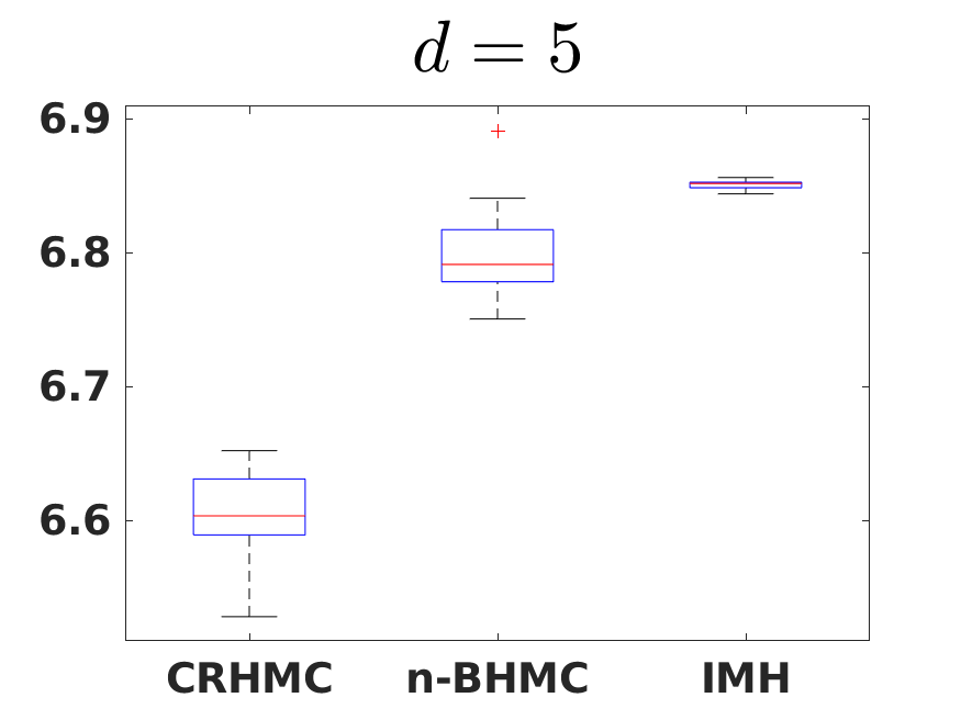
We evaluate their performance by taking as ground truth the estimate given by (i) the Metropolis-Adjusted Langevin Algorithm (MALA) (Roberts & Stramer 2002) for the hypercube and (ii) the Independent MH (IMH) algorithm (Liu 1996) for the simplex, which are also run 10 times, but 10 times longer than n-BHMC and CRHMC, i.e., for N=106N=10^{6} iterations. To compute the target quantity QQ, we keep the whole trajectories and report the confidence intervals in Figure 2. For both polytopes, we notably observe that our method is less biased than CRHMC.

Model dd NNZ n-BHMC CRHMC
ecoli 95 291 0.08822 5.719
cardiac-mit 220 228 0.1905 5.304
Aci-D21 851 1758 141.9 46.17
Aci-MR95 994 2859 325.1 61.34
Abi-49176 1069 2951 179.4 74.22
Aci-20731 1090 2946 0.7124 88.82
Aci-PHEA 1561 4640 2.343 100.8
iAF1260 2382 6368 537.9 170.5
iJO1366 2583 7284 537.9 169.4
Recon1 3742 8717 3.740 3280

Table 1: Real-world data setting: comparison with Kook et al. 2022a.

Real-world data.

We then consider 10 polytopes given in the COBRA Toolbox v3.0 (Heirendt et al. 2019), which model molecular systems, and follow the method provided in (Kook et al. 2022a, Appendix A) to pre-process them. Here, we aim at uniformly sampling from these polytopes. However, we do not have access to a realistic baseline that yields an unbiased estimator, since the sampling dimension is too high and running MALA or IMH would be too costly. Hence, instead of assessing the bias of the algorithms, we rather want to highlight that the “involution checking step” does not hurt the convergence properties of BHMC compared to CRHMC. We evaluate the efficiency of the algorithms by computing the sampling time per effective sample (in seconds), defined as the total sampling time until termination divided by the Effective Sample Size. We set the initial step-size to 0.01 for both algorithms and η=10\eta=10 in n-BHMC. We then follow the exact same procedure as in (Kook et al. 2022a, Table 1) by drawing 1000 uniform samples with limit on running time set to 1 day. Results are given in Table 1. For each molecular model, we specify by NNZ the number of non-zero entries in the matrix A\mathrm{A} defining the corresponding pre-processed polytope, which thus reflects its complexity. In particular, the sampling dimension dd corresponds to the number of columns of A\mathrm{A}. Note that the sampling time values are not of interest in themselves, but are only meant to compare CRHMC and n-BHMC. While it is clear that adding an “involution checking step” implies a trade-off between accuracy and complexity of the method, our results demonstrate that it does not penalize BHMC in the considered settings, and may even make it more efficient in some cases.

7 Discussion

In this paper, we introduced a novel version of RMHMC, Barrier HMC (BHMC), which addresses the problem of sampling from a distribution π\pi over a constrained convex subset 𝖬⊂ℝd\mathsf{M}\subset\mathbb{R}^{d} equipped with a self-concordant barrier ϕ\phi. Our contribution highlights that the use of well known implicit schemes for ODE integration combined with these space constraints leads to asymptotic bias when it comes to their numerical implementation. We propose to solve it in a straightforward manner via our algorithm, n-BHMC, which relies on an additional “involution checking step”. Under reasonable assumptions, our theory shows that this critical step removes the asymptotic bias. This result is supported by numerical experiments where we highlight this lack of bias compared to state-of-the-art methods. In future work, we would like to investigate the “coupled” behaviour of the hyperparameters hh and η\eta in practice, the study of irreductiblity of n-BHMC and the influence of η\eta on the bias. Moreover, we are interested in the application of n-BHMC for efficient polytope volume computation. More generally, we are convinced that our study is a first step for future work on designing implicit integration schemes for unbiased constrained sampling methods.

Acknowledgments

AD acknowledges support from the Lagrange Mathematics and Computing Research Center. AD and MN would like to thank the Isaac Newton Institute for Mathematical Sciences for support and hospitality during the programme The mathematical and statistical foundation of future data-driven engineering when work on this paper was undertaken. MN acknowledges funding from the grant SCAI (ANR-19-CHIA-0002).

References

  • Betancourt (2013) Betancourt, M. A general metric for Riemannian manifold Hamiltonian Monte Carlo. In International Conference on Geometric Science of Information, pp. 327–334. Springer, 2013.
  • Betancourt (2017) Betancourt, M. A conceptual introduction to Hamiltonian Monte Carlo. arXiv preprint arXiv:1701.02434, 2017.
  • Brofos & Lederman (2021a) Brofos, J. and Lederman, R. R. Evaluating the implicit midpoint integrator for Riemannian Hamiltonian Monte Carlo. In International Conference on Machine Learning, pp. 1072–1081. PMLR, 2021a.
  • Brofos & Lederman (2021b) Brofos, J. A. and Lederman, R. R. On numerical considerations for Riemannian Manifold Hamiltonian Monte Carlo. arXiv preprint arXiv:2111.09995, 2021b.
  • Brubaker et al. (2012) Brubaker, M., Salzmann, M., and Urtasun, R. A family of MCMC methods on implicitly defined manifolds. In Artificial Intelligence and Statistics, pp. 161–172. PMLR, 2012.
  • Bubeck et al. (2015) Bubeck, S., Eldan, R., and Lehec, J. Finite-time analysis of projected Langevin Monte Carlo. In Proceedings of the 28th International Conference on Neural Information Processing Systems, NIPS’15, pp. 1243–1251, Cambridge, MA, USA, 2015. MIT Press. URL http://dl.acm.org/citation.cfm?id=2969239.2969378.
  • Byrne & Girolami (2013) Byrne, S. and Girolami, M. Geodesic Monte Carlo on embedded manifolds. Scandinavian Journal of Statistics, 40(4):825–845, 2013.
  • Cobb et al. (2019) Cobb, A. D., Baydin, A. G., Markham, A., and Roberts, S. J. Introducing an explicit symplectic integration scheme for Riemannian Manifold Hamiltonian Monte Carlo. arXiv preprint arXiv:1910.06243, 2019.
  • Cousins & Vempala (2014) Cousins, B. and Vempala, S. Gaussian Cooling and O*(nˆ3) Algorithms for Volume and Gaussian Volume. ArXiv e-prints, September 2014.
  • Dalalyan (2017) Dalalyan, A. S. Theoretical guarantees for approximate sampling from smooth and log-concave densities. Journal of the Royal Statistical Society, Series B, 79(3):651–676, 2017.
  • Douc et al. (2018) Douc, R., Moulines, E., Priouret, P., and Soulier, P. Markov Chains. Springer, 2018.
  • Duane et al. (1987) Duane, S., Kennedy, A. D., Pendleton, B. J., and Roweth, D. Hybrid Monte Carlo. Physics letters B, 195(2):216–222, 1987.
  • Durmus & Moulines (2017) Durmus, A. and Moulines, E. Nonasymptotic convergence analysis for the unadjusted Langevin algorithm. The Annals of Applied Probability, 27(3):1551–1587, 06 2017. doi: 10.1214/16-AAP1238.
  • Dyer & Frieze (1991) Dyer, M. and Frieze, A. Computing the volume of convex bodies: a case where randomness provably helps. Probabilistic combinatorics and its applications, 44:123–170, 1991.
  • Gelfand et al. (1992) Gelfand, A. E., Smith, A. F., and Lee, T.-M. Bayesian analysis of constrained parameter and truncated data problems using Gibbs sampling. Journal of the American Statistical Association, 87(418):523–532, 1992.
  • Girolami & Calderhead (2011) Girolami, M. and Calderhead, B. Riemann Manifold Langevin and Hamiltonian Monte Carlo methods. Journal of the Royal Statistical Society: Series B (Statistical Methodology), 73(2):123–214, 2011.
  • Hairer et al. (2006) Hairer, E., Hochbruck, M., Iserles, A., and Lubich, C. Geometric numerical integration. Oberwolfach Reports, 3(1):805–882, 2006.
  • Heirendt et al. (2019) Heirendt, L., Arreckx, S., Pfau, T., Mendoza, S. N., Richelle, A., Heinken, A., Haraldsdóttir, H. S., Wachowiak, J., Keating, S. M., Vlasov, V., et al. Creation and analysis of biochemical constraint-based models using the COBRA Toolbox v. 3.0. Nature protocols, 14(3):639–702, 2019.
  • Kannan & Narayanan (2009) Kannan, R. and Narayanan, H. Random walks on polytopes and an affine interior point method for linear programming. In Proceedings of the forty-first annual ACM symposium on Theory of computing, pp. 561–570, 2009.
  • Kook et al. (2022a) Kook, Y., Lee, Y.-T., Shen, R., and Vempala, S. Sampling with Riemannian Hamiltonian Monte Carlo in a constrained space. Advances in Neural Information Processing Systems, 35:31684–31696, 2022a.
  • Kook et al. (2022b) Kook, Y., Lee, Y. T., Shen, R., and Vempala, S. S. Condition-number-independent convergence rate of Riemannian Hamiltonian Monte Carlo with numerical integrators. arXiv preprint arXiv:2210.07219, 2022b.
  • Lan & Shahbaba (2015) Lan, S. and Shahbaba, B. Sampling constrained probability distributions using Spherical Augmentation. ArXiv e-prints, June 2015.
  • Lee (2006) Lee, J. M. Riemannian Manifolds: an introduction to curvature, volume 176. Springer Science & Business Media, 2006.
  • Lee & Vempala (2017a) Lee, Y. T. and Vempala, S. S. Eldan’s stochastic localization and the KLS hyperplane conjecture: an improved lower bound for expansion. In 2017 IEEE 58th Annual Symposium on Foundations of Computer Science (FOCS), pp. 998–1007. IEEE, 2017a.
  • Lee & Vempala (2017b) Lee, Y. T. and Vempala, S. S. Geodesic walks in polytopes. In Proceedings of the 49th Annual ACM SIGACT Symposium on theory of Computing, pp. 927–940, 2017b.
  • Lee & Vempala (2018) Lee, Y. T. and Vempala, S. S. Convergence rate of Riemannian Hamiltonian Monte Carlo and faster polytope volume computation. In Proceedings of the 50th Annual ACM SIGACT Symposium on Theory of Computing, pp. 1115–1121, 2018.
  • Leimkuhler & Skeel (1994) Leimkuhler, B. J. and Skeel, R. D. Symplectic numerical integrators in constrained Hamiltonian systems. Journal of Computational Physics, 112(1):117–125, 1994.
  • Lelièvre et al. (2019) Lelièvre, T., Rousset, M., and Stoltz, G. Hybrid Monte Carlo methods for sampling probability measures on submanifolds. Numerische Mathematik, 143(2):379–421, 2019.
  • Lelièvre et al. (2022) Lelièvre, T., Stoltz, G., and Zhang, W. Multiple projection Markov Chain Monte Carlo algorithms on submanifolds. IMA Journal of Numerical Analysis, 2022.
  • Lewis et al. (2012) Lewis, N. E., Nagarajan, H., and Palsson, B. O. Constraining the metabolic genotype–phenotype relationship using a phylogeny of in silico methods. Nature Reviews Microbiology, 10(4):291–305, 2012.
  • Liu (1996) Liu, J. S. Metropolized independent sampling with comparisons to rejection sampling and importance sampling. Statistics and computing, 6:113–119, 1996.
  • Liu & Liu (2001) Liu, J. S. and Liu, J. S. Monte Carlo strategies in scientific computing, volume 10. Springer, 2001.
  • Lovász & Kannan (1999) Lovász, L. and Kannan, R. Faster mixing via average conductance. In Proceedings of the thirty-first annual ACM symposium on Theory of computing, pp. 282–287. ACM, 1999.
  • Lovász & Simonovits (1993) Lovász, L. and Simonovits, M. Random walks in a convex body and an improved volume algorithm. Random structures & algorithms, 4(4):359–412, 1993.
  • Lovász & Vempala (2004) Lovász, L. and Vempala, S. Hit-and-run from a corner. In Proceedings of the thirty-sixth annual ACM symposium on Theory of computing, pp. 310–314, 2004.
  • Lovász & Vempala (2007) Lovász, L. and Vempala, S. The geometry of logconcave functions and sampling algorithms. Random Struct. Algorithms, 30(3):307–358, May 2007. ISSN 1042-9832. doi: 10.1002/rsa.v30:3. URL http://dx.doi.org/10.1002/rsa.v30:3.
  • Mok (1977) Mok, K.-P. Metrics and connections on the cotangent bundle. In Kodai Mathematical Seminar Reports, volume 28, pp. 226–238. Department of Mathematics, Tokyo Institute of Technology, 1977.
  • Morris (2002) Morris, B. J. Improved bounds for sampling contingency tables. Random Structures & Algorithms, 21(2):135–146, 2002.
  • Neal et al. (2011) Neal, R. M. et al. MCMC using Hamiltonian dynamics. Handbook of Markov Chain Monte Carlo, 2(11):2, 2011.
  • Nesterov (2003) Nesterov, Y. Introductory lectures on convex optimization: A basic course, volume 87. Springer Science & Business Media, 2003.
  • Nesterov & Nemirovski (1998) Nesterov, Y. and Nemirovski, A. Multi-parameter surfaces of analytic centers and long-step surface-following interior point methods. Mathematics of Operations Research, 23(1):1–38, 1998.
  • Nesterov & Nemirovskii (1994) Nesterov, Y. and Nemirovskii, A. Interior-point polynomial algorithms in convex programming. SIAM, 1994.
  • Pakman & Paninski (2014) Pakman, A. and Paninski, L. Exact Hamiltonian Monte Carlo for truncated multivariate Gaussians. Journal of Computational and Graphical Statistics, 23(2):518–542, 2014.
  • Roberts & Rosenthal (2001) Roberts, G. O. and Rosenthal, J. S. Optimal scaling for various Metropolis-Hastings algorithms. Statistical science, 16(4):351–367, 2001.
  • Roberts & Stramer (2002) Roberts, G. O. and Stramer, O. Langevin diffusions and Metropolis-Hastings algorithms. Methodology and computing in applied probability, 4:337–357, 2002.
  • Sasaki (1958) Sasaki, S. On the differential geometry of tangent bundles of Riemannian manifolds. Tohoku Mathematical Journal, Second Series, 10(3):338–354, 1958.
  • Shahbaba et al. (2014) Shahbaba, B., Lan, S., Johnson, W. O., and Neal, R. M. Split Hamiltonian Monte Carlo. Statistics and Computing, 24(3):339–349, 2014.
  • Strang (1968) Strang, G. On the construction and comparison of difference schemes. SIAM Journal on Numerical Analysis, 5(3):506–517, 1968.
  • Tao (2016) Tao, M. Explicit symplectic approximation of nonseparable Hamiltonians: Algorithm and long time performance. Physical Review E, 94(4):043303, 2016.
  • Thiele et al. (2013) Thiele, I., Swainston, N., Fleming, R. M., Hoppe, A., Sahoo, S., Aurich, M. K., Haraldsdottir, H., Mo, M. L., Rolfsson, O., Stobbe, M. D., et al. A community-driven global reconstruction of human metabolism. Nature biotechnology, 31(5):419–425, 2013.
  • Zappa et al. (2018) Zappa, E., Holmes-Cerfon, M., and Goodman, J. Monte Carlo on manifolds: sampling densities and integrating functions. Communications on Pure and Applied Mathematics, 71(12):2609–2647, 2018.

Organisation of the supplementary

This appendix is organized as follows. Appendix A summarizes general facts that will be useful for proofs. Appendix B and Appendix C provide additional details on Riemannian metrics and technicalities on self-concordance, respectively. The c-BHMC algorithm is presented in Appendix D with some results whose proofs are given in Appendix E. Appendix F presents general facts about numerical integration and specific facts on the integrators used in n-BHMC. Appendix G dispenses the proof of the result on implicit integrators of n-BHMC, stated in Section 4.1. Appendix H presents the modified version of n-BHMC, incorporating a step-size condition, for which we state the reversibility with respect to the target distribution in Section 4.2. Proof of this last result is given in Appendix I. A detailed comparison between n-BHMC and CRHMC (Kook et al. 2022a) is given in Appendix J. Finally, Appendix K provides more details on the experiments of Section 6.

Notation.

For any Riemannian manifold (𝖬,𝔤)(\mathsf{M},\mathfrak{g}) and any z=(x,p)∈T⋆​𝖬z=(x,p)\in\mathrm{T}^{\star}\mathsf{M}, we denote by ∥⋅∥z\|\cdot\|_{z} the norm (20) defined on T⋆​𝖬\mathrm{T}^{\star}\mathsf{M} by ‖(x′,p′)‖z=‖x′‖𝔤⁡(x)+‖p′‖𝔤​(x)−1\|(x^{\prime},p^{\prime})\|_{z}=\|x^{\prime}\|_{\mathfrak{g}(x)}+\|p^{\prime}\|_{\mathfrak{g}(x)^{-1}} for any (x′,p′)∈T⋆​𝖬(x^{\prime},p^{\prime})\in\mathrm{T}^{\star}\mathsf{M}. For any open subset 𝖴⊂ℝd\mathsf{U}\subset\mathbb{R}^{d} and any k∈ℕk\in\mathbb{N}, we denote by Ck​(𝖴,ℝd′)\mathrm{C}^{k}(\mathsf{U},\mathbb{R}^{d^{\prime}}) the set of functions f:𝖴→ℝd′f:\mathsf{U}\to\mathbb{R}^{d^{\prime}} such that ff is kk times continuously differentiable.

Appendix A Useful facts and lemmas

We recall here some basic knowledge on linear algebra and probability, and state useful inequalities for our proofs.

Linear algebra reminders.

For any matrices A,B∈ℝd×d\mathrm{A},\mathrm{B}\in\mathbb{R}^{d\times d}, we write A⪯B\mathrm{A}\preceq\mathrm{B} if for any x∈ℝdx\in\mathbb{R}^{d}, x⊤​(B−A)​x≥0x^{\top}(\mathrm{B}-\mathrm{A})x\geq 0. Any positive-definite matrix A∈ℝd×d\mathrm{A}\in\mathbb{R}^{d\times d} induces a scalar product ⟨⋅,⋅⟩A\langle\cdot,\cdot\rangle_{\mathrm{A}} on ℝd\mathbb{R}^{d}, defined by ⟨x,y⟩A=⟨x,A​y⟩\langle x,y\rangle_{\mathrm{A}}=\langle x,\mathrm{A}y\rangle. This scalar product induces the norm ∥⋅∥A\|\cdot\|_{\mathrm{A}} on ℝd\mathbb{R}^{d}, defined by ‖x‖A=⟨x,x⟩A=‖A1/2​x‖2\|x\|_{\mathrm{A}}=\sqrt{\langle x,x\rangle_{\mathrm{A}}}=\|\mathrm{A}^{1/2}x\|_{2}. For any positive-definite matrices A,B∈ℝd×d\mathrm{A},\mathrm{B}\in\mathbb{R}^{d\times d} and for any α≥0\alpha\geq 0, A⪯α​B\mathrm{A}\preceq\alpha\mathrm{B} is equivalent to ∥⋅∥A≤α∥⋅∥B\|\cdot\|_{\mathrm{A}}\leq\sqrt{\alpha}\|\cdot\|_{\mathrm{B}}. The canonical norm of ℝd\mathbb{R}^{d} induces the norm ∥⋅∥2\|\cdot\|_{2} on ℝd×d\mathbb{R}^{d\times d}, defined by ‖A‖2=sup‖u‖2=1‖A​u‖2\|\mathrm{A}\|_{2}=\sup_{\|u\|_{2}=1}\|\mathrm{A}u\|_{2}. In particular, for any matrices A,B∈ℝd×d\mathrm{A},\mathrm{B}\in\mathbb{R}^{d\times d} and any vector x∈ℝdx\in\mathbb{R}^{d}, ‖A​x‖2≤‖A‖2​‖x‖2\|\mathrm{A}x\|_{2}\leq\|\mathrm{A}\|_{2}\|x\|_{2} and ‖AB‖2≤‖A‖2​‖B‖2\|\mathrm{A}\mathrm{B}\|_{2}\leq\|\mathrm{A}\|_{2}\|\mathrm{B}\|_{2}. Moreover, if A\mathrm{A} is non-negative-definite, then ‖A‖2=λ⁡(A)\|\mathrm{A}\|_{2}=\lambda(\mathrm{A}), where λ⁡(A)\lambda(\mathrm{A}) is the largest eigenvalue of A\mathrm{A}, and ‖Aα‖2=λ​(A)α\|\mathrm{A}^{\alpha}\|_{2}=\lambda(\mathrm{A})^{\alpha} for any α>0\alpha>0.

Probability reminders.

In this section, we consider a smooth manifold 𝖬⊂ℝd\mathsf{M}\subset\mathbb{R}^{d}. We first recall the definition of reversibility (Douc et al. 2018, Definition 1.5.1) before stating general results on reversibility.

Definition 4.

Let Q:T⋆​𝖬×ℬ⁡(T⋆​𝖬)→[0,1]\mathrm{Q}:\mathrm{T}^{\star}\mathsf{M}\times\mathcal{B}(\mathrm{T}^{\star}\mathsf{M})\rightarrow\left[0,1\right] be a transition probability kernel and let π¯\bar{\pi} be a probability distribution on T⋆​𝖬\mathrm{T}^{\star}\mathsf{M}. Then,

  1. (a)

    Q\mathrm{Q} is said to be reversible with respect to π¯\bar{\pi} if for any f∈C⁡(T⋆​𝖬×T⋆​𝖬,ℝ)f\in\mathrm{C}(\mathrm{T}^{\star}\mathsf{M}\times\mathrm{T}^{\star}\mathsf{M},\mathbb{R}) with compact support

    ∫T⋆​𝖬×T⋆​𝖬f⁡(z,z′)​Q​(z,d​z′)​π¯​(𝑑z)=∫T⋆​𝖬×T⋆​𝖬f⁡(z′,z)​Q​(z,d​z′)​π¯​(𝑑z).\displaystyle\textstyle{\int_{\mathrm{T}^{\star}\mathsf{M}\times\mathrm{T}^{\star}\mathsf{M}}f(z,z^{\prime})\mathrm{Q}(z,\mathrm{d}z^{\prime})\bar{\pi}(\mathrm{d}z)=\int_{\mathrm{T}^{\star}\mathsf{M}\times\mathrm{T}^{\star}\mathsf{M}}f(z^{\prime},z)\mathrm{Q}(z,\mathrm{d}z^{\prime})\bar{\pi}(\mathrm{d}z)\;.} (28)
  2. (b)

    Q\mathrm{Q} is said to be reversible up to momentum reversal with respect to π¯\bar{\pi} if for any f∈C⁡(T⋆​𝖬×T⋆​𝖬,ℝ)f\in\mathrm{C}(\mathrm{T}^{\star}\mathsf{M}\times\mathrm{T}^{\star}\mathsf{M},\mathbb{R}) with compact support

    ∫T⋆​𝖬×T⋆​𝖬f⁡(z,z′)​Q​(z,d​z′)​π¯​(𝑑z)=∫T⋆​𝖬×T⋆​𝖬f⁡(s⁡(z′),s⁡(z))​Q​(z,d​z′)​π¯​(𝑑z),\displaystyle\textstyle{\int_{\mathrm{T}^{\star}\mathsf{M}\times\mathrm{T}^{\star}\mathsf{M}}f(z,z^{\prime})\mathrm{Q}(z,\mathrm{d}z^{\prime})\bar{\pi}(\mathrm{d}z)=\int_{\mathrm{T}^{\star}\mathsf{M}\times\mathrm{T}^{\star}\mathsf{M}}f(s(z^{\prime}),s(z))\mathrm{Q}(z,\mathrm{d}z^{\prime})\bar{\pi}(\mathrm{d}z)\;,} (29)

    where we recall that for any (x,p)∈ℝd×ℝd(x,p)\in\mathbb{R}^{d}\times\mathbb{R}^{d}, s⁡(x,p)=(x,−p)s(x,p)=(x,-p).

Lemma 5.

Let Q:T⋆​𝖬×ℬ⁡(T⋆​𝖬)→[0,1]\mathrm{Q}:\mathrm{T}^{\star}\mathsf{M}\times\mathcal{B}(\mathrm{T}^{\star}\mathsf{M})\rightarrow\left[0,1\right] be a transition probability kernel and let π¯\bar{\pi} be a probability distribution on T⋆​𝖬\mathrm{T}^{\star}\mathsf{M}. Assume that s#​π¯=π¯s_{\#}\bar{\pi}=\bar{\pi} and that Q\mathrm{Q} is reversible up to momentum reversal with respect to π¯\bar{\pi}. Then π¯\bar{\pi} is an invariant measure for Q\mathrm{Q}, i.e., for any f∈C⁡(T⋆​𝖬,ℝ)f\in\mathrm{C}(\mathrm{T}^{\star}\mathsf{M},\mathbb{R}) with compact support

∫T⋆​𝖬×T⋆​𝖬f⁡(z′)​Q​(z,d​z′)​π¯​(𝑑z)=∫T⋆​𝖬×T⋆​𝖬f⁡(z)​π¯​(𝑑z).\displaystyle\textstyle{\int_{\mathrm{T}^{\star}\mathsf{M}\times\mathrm{T}^{\star}\mathsf{M}}f(z^{\prime})\mathrm{Q}(z,\mathrm{d}z^{\prime})\bar{\pi}(\mathrm{d}z)=\int_{\mathrm{T}^{\star}\mathsf{M}\times\mathrm{T}^{\star}\mathsf{M}}f(z)\bar{\pi}(\mathrm{d}z)\;.} (30)
Proof.

Let f∈C⁡(T⋆​𝖬,ℝ)f\in\mathrm{C}(\mathrm{T}^{\star}\mathsf{M},\mathbb{R}) with compact support. We have

∫T⋆​𝖬×T⋆​𝖬f⁡(z′)​Q​(z,d​z′)​π¯​(𝑑z)\displaystyle\textstyle{\int_{\mathrm{T}^{\star}\mathsf{M}\times\mathrm{T}^{\star}\mathsf{M}}f(z^{\prime})\mathrm{Q}(z,\mathrm{d}z^{\prime})\bar{\pi}(\mathrm{d}z)} (31)
=∫T⋆​𝖬×T⋆​𝖬f⁡(s⁡(z))​Q​(z,d​z′)​π¯​(𝑑z)\displaystyle\qquad=\textstyle{\int_{\mathrm{T}^{\star}\mathsf{M}\times\mathrm{T}^{\star}\mathsf{M}}f(s(z))\mathrm{Q}(z,\mathrm{d}z^{\prime})\bar{\pi}(\mathrm{d}z)} (Appendix A) (32)
=∫T⋆​𝖬×T⋆​𝖬f⁡(z)​Q​(s⁡(z),d​z′)​(s#​π¯)​(𝑑z)=∫T⋆​𝖬f⁡(z)​π¯​(𝑑z)\displaystyle\qquad=\textstyle{\int_{\mathrm{T}^{\star}\mathsf{M}\times\mathrm{T}^{\star}\mathsf{M}}f(z)\mathrm{Q}(s(z),\mathrm{d}z^{\prime})(s_{\#}\bar{\pi})(\mathrm{d}z)=\int_{\mathrm{T}^{\star}\mathsf{M}}f(z)\bar{\pi}(\mathrm{d}z)} (momentum reversal on z),\displaystyle\text{(momentum reversal on $z$)}\;, (33)

which concludes the proof. ∎

Lemma 6.

Let Q:T⋆​𝖬×ℬ⁡(T⋆​𝖬)→[0,1]\mathrm{Q}:\mathrm{T}^{\star}\mathsf{M}\times\mathcal{B}(\mathrm{T}^{\star}\mathsf{M})\rightarrow\left[0,1\right] be a transition probability kernel and let π¯\bar{\pi} be a probability distribution on T⋆​𝖬\mathrm{T}^{\star}\mathsf{M}. Assume that s#​Q=Qs_{\#}\mathrm{Q}=\mathrm{Q} and that Q\mathrm{Q} is reversible with respect to π¯\bar{\pi}. Then, Q\mathrm{Q} is reversible up to momentum reversal with respect to π¯\bar{\pi}.

Proof.

Let f∈C⁡(T⋆​𝖬,ℝ)f\in\mathrm{C}(\mathrm{T}^{\star}\mathsf{M},\mathbb{R}) with compact support. We have

∫T⋆​𝖬×T⋆​𝖬f⁡(z,z′)​Q​(z,d​z′)​π¯​(𝑑z)\displaystyle\textstyle{\int_{\mathrm{T}^{\star}\mathsf{M}\times\mathrm{T}^{\star}\mathsf{M}}f(z,z^{\prime})\mathrm{Q}(z,\mathrm{d}z^{\prime})\bar{\pi}(\mathrm{d}z)} (34)
=∫T⋆​𝖬×T⋆​𝖬f⁡(z,s⁡(z′))​(s#​Q)​(z,d​z′)​π¯​(𝑑z)\displaystyle\qquad=\textstyle{\int_{\mathrm{T}^{\star}\mathsf{M}\times\mathrm{T}^{\star}\mathsf{M}}f(z,s(z^{\prime}))(s_{\#}\mathrm{Q})(z,\mathrm{d}z^{\prime})\bar{\pi}(\mathrm{d}z)} (momentum reversal on z′z^{\prime}) (35)
=∫T⋆​𝖬×T⋆​𝖬f⁡(z′,s⁡(z))​Q​(z,d​z′)​π¯​(𝑑z)\displaystyle\qquad=\textstyle{\int_{\mathrm{T}^{\star}\mathsf{M}\times\mathrm{T}^{\star}\mathsf{M}}f(z^{\prime},s(z))\mathrm{Q}(z,\mathrm{d}z^{\prime})\bar{\pi}(\mathrm{d}z)} (Appendix A) (36)
=∫T⋆​𝖬×T⋆​𝖬f⁡(s⁡(z′),s⁡(z))​(s#​Q)​(z,d​z′)​π¯​(𝑑z)\displaystyle\qquad=\textstyle{\int_{\mathrm{T}^{\star}\mathsf{M}\times\mathrm{T}^{\star}\mathsf{M}}f(s(z^{\prime}),s(z))(s_{\#}\mathrm{Q})(z,\mathrm{d}z^{\prime})\bar{\pi}(\mathrm{d}z)} (momentum reversal on z′z^{\prime}) (37)
=∫T⋆​𝖬×T⋆​𝖬f⁡(s⁡(z′),s⁡(z))​Q​(z,d​z′)​π¯​(𝑑z),\displaystyle\qquad=\textstyle{\int_{\mathrm{T}^{\star}\mathsf{M}\times\mathrm{T}^{\star}\mathsf{M}}f(s(z^{\prime}),s(z))\mathrm{Q}(z,\mathrm{d}z^{\prime})\bar{\pi}(\mathrm{d}z)}\;, (38)

which concludes the proof. ∎

Useful inequalities.

The following inequalities hold:

  1. (a)

    For any u∈[0,1/5]u\in[0,1/5], (1−u)−2≤1+3​u(1-u)^{-2}\leq 1+3u and (1−u)−3≤1+5​u(1-u)^{-3}\leq 1+5u.

  2. (b)

    For any u∈[0,1/2]u\in[0,1/2], (1−u)−1≤1+2​u(1-u)^{-1}\leq 1+2u.

  3. (c)

    For any u∈[0,1]u\in[0,1], |(1−u)2−1|≤3​u|(1-u)^{2}-1|\leq 3u.

  4. (d)

    For any u≥0u\geq 0, we have 1−(1+u)−1≤u1-(1+u)^{-1}\leq u and (1−u)2−1≥−2​u(1-u)^{2}-1\geq-2u.

Appendix B Details on Riemannian metrics

Let 𝖬\mathsf{M} be a smooth dd-dimensional manifold, endowed with a metric 𝔤\mathfrak{g}. We recall that the Riemannian volume element corresponding to (𝖬,𝔤)(\mathsf{M},\mathfrak{g}) is given in local coordinates by dvol𝖬​(x)=det(𝔤)​d​x\mathrm{d}\mathrm{vol}_{\mathsf{M}}(x)=\sqrt{\det(\mathfrak{g})}\mathrm{d}x, where d​x\mathrm{d}x is a dual coframe, (Lee 2006, Lemma 3.2.). For any x∈𝖬x\in\mathsf{M}, we respectively denote by Tx​𝖬\mathrm{T}_{x}\mathsf{M} and Tx⋆​𝖬\mathrm{T}_{x}^{\star}\mathsf{M}, the tangent space at xx and its dual space, i.e., the cotangent space at xx. Note that Tx​𝖬\mathrm{T}_{x}\mathsf{M} and Tx⋆​𝖬\mathrm{T}_{x}^{\star}\mathsf{M} are space vectors, and Tx​𝖬\mathrm{T}_{x}\mathsf{M} is endowed with the scalar product ⟨⋅,⋅⟩𝔤⁡(x)\langle\cdot,\cdot\rangle_{\mathfrak{g}(x)} by definition of the Riemannian metric. For clarity sake, we denote by vv (resp. pp) an element of the tangent (resp. cotangent) space. We recall that the tangent bundle T​𝖬\mathrm{T}\mathsf{M} and the cotangent bundle T⋆​𝖬\mathrm{T}^{\star}\mathsf{M} are respectively defined by T𝖬=⊔x∈𝖬{x}∪Tx𝖬\mathrm{T}\mathsf{M}=\sqcup_{x\in\mathsf{M}}\{x\}\cup\mathrm{T}_{x}\mathsf{M} and T⋆𝖬=⊔x∈𝖬{x}∪Tx⋆𝖬\mathrm{T}^{\star}\mathsf{M}=\sqcup_{x\in\mathsf{M}}\{x\}\cup\mathrm{T}_{x}^{\star}\mathsf{M}. These two sets are 2​d2d-dimensional manifolds.

Metric on the tangent bundle T​𝖬\mathrm{T}\mathsf{M}.

Sasaki 1958 originally introduced on T​𝖬\mathrm{T}\mathsf{M} a Riemannian metric 𝔤^\hat{\mathfrak{g}}, which, among other properties, preserves the Euclidean metric induced by 𝔤\mathfrak{g} on each tangent space. This metric is defined by

𝔤^=(𝔤i​j+vk​vl​Γi​sk​Γt​jl​𝔤s​t−𝔤j​s​vk​Γi​sk−𝔤i​s​vk​Γj​sk𝔤i​j),\hat{\mathfrak{g}}=\begin{pmatrix}\mathfrak{g}_{ij}+v^{k}v^{l}\Gamma^{k}_{is}\Gamma_{tj}^{l}\mathfrak{g}^{st}&-\mathfrak{g}^{js}v^{k}\Gamma_{is}^{k}\\ -\mathfrak{g}^{is}v^{k}\Gamma_{js}^{k}&\mathfrak{g}_{ij}\end{pmatrix}\;, (39)

where 𝔤i​j\mathfrak{g}_{ij} and 𝔤i​j\mathfrak{g}^{ij} respectively refer to 𝔤\mathfrak{g} and 𝔤−1\mathfrak{g}^{-1}, and Γ\Gamma corresponds to the Christoffel symbol. Since (T​𝖬,𝔤^)(\mathrm{T}\mathsf{M},\hat{\mathfrak{g}}) is a Riemannian manifold, the volume form on T​𝖬\mathrm{T}\mathsf{M} satisfies for any (x,v)∈T​𝖬(x,v)\in\mathrm{T}\mathsf{M}

dvolT​𝖬​(x,v)=det(𝔤^​(x,v))​d​x​d​v=det(𝔤⁡(x))​d​x​d​v.\mathrm{d}\mathrm{vol}_{\mathrm{T}\mathsf{M}}(x,v)=\sqrt{\det(\hat{\mathfrak{g}}(x,v))}\mathrm{d}x\mathrm{d}v=\det(\mathfrak{g}(x))\mathrm{d}x\mathrm{d}v\;. (40)

Metric on the cotangent bundle T⋆​𝖬\mathrm{T}^{\star}\mathsf{M}.

Elaborating on the metric defined by Sasaki 1958, Mok 1977 showed that for any x∈𝖬x\in\mathsf{M}, Tx⋆​𝖬\mathrm{T}_{x}^{\star}\mathsf{M} is naturally endowed with the scalar product ⟨⋅,⋅⟩𝔤​(x)−1\langle\cdot,\cdot\rangle_{\mathfrak{g}(x)^{-1}}, and proposed a Riemannian metric 𝔤⋆\mathfrak{g}^{\star} on T⋆​𝖬\mathrm{T}^{\star}\mathsf{M}, which notably preserves this result on each cotangent space. This metric is closely related to 𝔤^\hat{\mathfrak{g}} and is defined by

𝔤⋆=(𝔤i​j+pk​pl​Γi​sk​Γt​jl​𝔤s​t−𝔤j​s​pk​Γi​sk−𝔤i​s​pk​Γj​sk𝔤i​j).\mathfrak{g}^{\star}=\begin{pmatrix}\mathfrak{g}_{ij}+p^{k}p^{l}\Gamma^{k}_{is}\Gamma_{tj}^{l}\mathfrak{g}^{st}&-\mathfrak{g}^{js}p^{k}\Gamma_{is}^{k}\\ -\mathfrak{g}^{is}p^{k}\Gamma_{js}^{k}&\mathfrak{g}^{ij}\end{pmatrix}\;. (41)

Since (T⋆​𝖬,𝔤⋆)(\mathrm{T}^{\star}\mathsf{M},\mathfrak{g}^{\star}) is a Riemannian manifold, the volume form on T⋆​𝖬\mathrm{T}^{\star}\mathsf{M} satisfies for any (x,p)∈T⋆​𝖬(x,p)\in\mathrm{T}^{\star}\mathsf{M}

dvolT⋆​𝖬​(x,p)=det(𝔤⋆​(x,p))​d​x​d​p=d​x​d​p.\mathrm{d}\mathrm{vol}_{\mathrm{T}^{\star}\mathsf{M}}(x,p)=\sqrt{\det(\mathfrak{g}^{\star}(x,p))}\mathrm{d}x\mathrm{d}p=\mathrm{d}x\mathrm{d}p\;. (42)

In contrast to the tangent bundle, the volume form on the cotangent bundle does not depend on 𝔤\mathfrak{g}, which motivates to augment on T⋆​𝖬\mathrm{T}^{\star}\mathsf{M} (instead of T​𝖬\mathrm{T}\mathsf{M}) any target measure π\pi defined on 𝖬\mathsf{M}.

Appendix C Properties of self-concordance

We first recall the definition of self-concordance and derive some of its properties in Appendices C and C.

Definition 7 (Nesterov & Nemirovskii 1994).

Let 𝖴\mathsf{U} be a non-empty open convex domain in ℝd\mathbb{R}^{d}. A function ϕ:𝖴→ℝ\phi:\mathsf{U}\rightarrow\mathbb{R} is said to be a ν\nu-self-concordant barrier (with ν≥1\nu\geq 1) on 𝖴\mathsf{U} if it satisfies:

  1. (a)

    ϕ∈C3​(𝖴,ℝ)\phi\in\mathrm{C}^{3}(\mathsf{U},\mathbb{R}) and ϕ\phi is convex,

  2. (b)

    ϕ⁡(x)→+∞\phi(x)\xrightarrow{}+\infty as x→∂𝖴x\rightarrow\partial\mathsf{U},

  3. (c)

    |D3​ϕ​(x)​[h,h,h]|≤2​‖h‖𝔤⁡(x)3|D^{3}\phi(x)[h,h,h]|\leq 2\|h\|_{\mathfrak{g}(x)}^{3}, for any x∈𝖬x\in\mathsf{M}, h∈ℝdh\in\mathbb{R}^{d},

  4. (d)

    |D​ϕ​(x)​[h]|2≤ν​‖h‖𝔤⁡(x)2|D\phi(x)[h]|^{2}\leq\nu\|h\|_{\mathfrak{g}(x)}^{2}, for any x∈𝖬x\in\mathsf{M}, h∈ℝdh\in\mathbb{R}^{d},

where 𝔤⁡(x)=D2​ϕ​(x)\mathfrak{g}(x)=D^{2}\phi(x).

Self-concordance can be thought as a certain kind of regularity. Indeed, if ϕ\phi is a ν\nu-self-concordant barrier on a convex body 𝖴\mathsf{U}, then D2​ϕD^{2}\phi is 22-Lipschitz continuous on 𝖴\mathsf{U} with respect to the local norm induced by 𝔤\mathfrak{g} (see Property (c)), and more restrictively, ϕ\phi is ν\nu-Lipschitz continuous with respect to the same norm (see Property (d)).

Lemma 8.

Let ϕ:𝖴→ℝ\phi:\mathsf{U}\rightarrow\mathbb{R} be a ν\nu-self-concordant barrier with 𝔤=D2​ϕ\mathfrak{g}=D^{2}\phi. Assume that 𝖴\mathsf{U} is bounded. Then, ‖∇ϕ​(x)‖2→+∞\|\nabla\phi(x)\|_{2}\xrightarrow{}+\infty and ‖𝔤⁡(x)‖2→+∞\|\mathfrak{g}(x)\|_{2}\xrightarrow{}+\infty as x→∂𝖴x\rightarrow\partial\mathsf{U}.

Proof.

Since ϕ\phi is convex, we have, for any (x,y)∈𝖴2(x,y)\in\mathsf{U}^{2}

ϕ⁡(x)\displaystyle\textstyle{\phi(x)} ≤ϕ⁡(y)+∇ϕ​(x)​(x−y),\displaystyle\textstyle{\leq\phi(y)+\nabla\phi(x)(x-y)\;,} (43)
|ϕ⁡(x)|\displaystyle\textstyle{|\phi(x)|} ≤|ϕ⁡(y)|+‖∇ϕ​(x)‖2​‖x−y‖2\displaystyle\textstyle{\leq|\phi(y)|+\|\nabla\phi(x)\|_{2}\|x-y\|_{2}} (44)
≤|ϕ⁡(y)|+‖∇ϕ​(x)‖2​diam⁡(𝖴),\displaystyle\textstyle{\leq|\phi(y)|+\|\nabla\phi(x)\|_{2}\operatorname{diam}(\mathsf{U})\;,} (45)

where we used Cauchy-Schwartz inequality in the second line. Using Property (b) of ϕ\phi, we obtain that ‖∇ϕ​(x)‖2→+∞\|\nabla\phi(x)\|_{2}\xrightarrow{}+\infty as x→∂𝖴x\rightarrow\partial\mathsf{U}. By combining this result with Property (d) of ϕ\phi, we obtain that ‖𝔤⁡(x)‖2→+∞\|\mathfrak{g}(x)\|_{2}\xrightarrow{}+\infty as x→∂𝖴x\rightarrow\partial\mathsf{U}. ∎

According to Nesterov 2003 (see Lemma 4.1.2), Property (c) of self-concordance is equivalent to

|D3​ϕ​(x)​[h1,h2,h3]|≤2​∏i=13‖hi‖𝔤⁡(x),\displaystyle\textstyle{|D^{3}\phi(x)[h_{1},h_{2},h_{3}]|\leq 2\prod_{i=1}^{3}\|h_{i}\|_{\mathfrak{g}(x)}\;,} (46)

for any x∈𝖬x\in\mathsf{M} and any (h1,h2,h3)∈ℝd×ℝd×ℝd(h_{1},h_{2},h_{3})\in\mathbb{R}^{d}\times\mathbb{R}^{d}\times\mathbb{R}^{d}.

Let u:ℝd→ℝdu:\ \mathbb{R}^{d}\to\mathbb{R}^{d} be a linear operator. For any x∈ℝdx\in\mathbb{R}^{d}, we define the operator norms ‖u‖𝔤⁡(x)\|u\|_{\mathfrak{g}(x)} and ‖u‖𝔤​(x)−1\|u\|_{\mathfrak{g}(x)^{-1}} by

‖u‖𝔤⁡(x)\displaystyle\|u\|_{\mathfrak{g}(x)} =sup{u⁡(𝔤⁡(x)​h):‖h‖𝔤⁡(x)=1},\displaystyle=\sup\{u(\mathfrak{g}(x)h)\,:\;\|h\|_{\mathfrak{g}(x)}=1\}\;, (47)
‖u‖𝔤​(x)−1\displaystyle\|u\|_{\mathfrak{g}(x)^{-1}} =sup{u⁡(𝔤​(x)−1​h):‖h‖𝔤​(x)−1=1}.\displaystyle=\sup\{u(\mathfrak{g}(x)^{-1}h)\,:\;\|h\|_{\mathfrak{g}(x)^{-1}}=1\}\;. (48)

In addition, a set 𝖵⊂ℝd\mathsf{V}\subset\mathbb{R}^{d} contains no straight line if for any 𝖣x0={t​x0:t∈ℝ}\mathsf{D}_{x_{0}}=\{tx_{0}\,:\;t\in\mathbb{R}\} with x0≠0x_{0}\neq 0, we have 𝖵c∩𝖣x0≠∅\mathsf{V}^{\mathrm{c}}\cap\mathsf{D}_{x_{0}}\neq\emptyset.

Lemma 9.

Let ϕ:𝖴→ℝ\phi:\mathsf{U}\rightarrow\mathbb{R} be a ν\nu-self-concordant barrier with 𝔤=D2​ϕ\mathfrak{g}=D^{2}\phi. Assume that 𝖴\mathsf{U} contains no straight line. For any x∈𝖴x\in\mathsf{U} and any r>0r>0, we denote by 𝖶0​(x,r)\mathsf{W}^{0}(x,r) the open Dikin ellipsoid of ϕ\phi at xx, given by 𝖶0​(x,r)={y∈ℝd∣‖y−x‖𝔤⁡(x)<r}\mathsf{W}^{0}(x,r)=\{y\in\mathbb{R}^{d}\mid\|y-x\|_{\mathfrak{g}(x)}<r\}. Then, the following properties hold:

  1. (a)

    For any x∈𝖴x\in\mathsf{U} and any (h1,h2)∈ℝd×ℝd(h_{1},h_{2})\in\mathbb{R}^{d}\times\mathbb{R}^{d}

    ‖D3​ϕ​(x)​[h1,h2]‖𝔤​(x)−1≤2​‖h1‖𝔤⁡(x)​‖h2‖𝔤⁡(x).\displaystyle\|D^{3}\phi(x)[h_{1},h_{2}]\|_{\mathfrak{g}(x)^{-1}}\leq 2\|h_{1}\|_{\mathfrak{g}(x)}\|h_{2}\|_{\mathfrak{g}(x)}\;. (49)
  2. (b)

    For any x∈𝖴x\in\mathsf{U}, 𝖶0​(x,1)⊂𝖴\mathsf{W}^{0}(x,1)\subset\mathsf{U}, and for any y∈𝖶0​(x,1)y\in\mathsf{W}^{0}(x,1)

    (1−‖y−x‖𝔤⁡(x))2​𝔤​(x)⪯𝔤⁡(y)⪯(1−‖y−x‖𝔤⁡(x))−2​𝔤​(x).\displaystyle(1-\|y-x\|_{\mathfrak{g}(x)})^{2}\mathfrak{g}(x)\preceq\mathfrak{g}(y)\preceq(1-\|y-x\|_{\mathfrak{g}(x)})^{-2}\mathfrak{g}(x)\;. (50)
  3. (c)

    For any x∈𝖴x\in\mathsf{U}, any y∈𝖶0​(x,1)y\in\mathsf{W}^{0}(x,1) and any h∈ℝdh\in\mathbb{R}^{d}, the following hold

    ‖h‖𝔤⁡(x)≤(1−‖y−x‖𝔤⁡(x))−1​‖h‖𝔤⁡(y),‖h‖𝔤⁡(y)≤(1−‖y−x‖𝔤⁡(x))−1​‖h‖𝔤⁡(x),‖h‖𝔤​(x)−1≤(1−‖y−x‖𝔤⁡(x))−1​‖h‖𝔤​(y)−1,‖h‖𝔤​(y)−1≤(1−‖y−x‖𝔤⁡(x))−1​‖h‖𝔤​(x)−1.\displaystyle\begin{split}&\|h\|_{\mathfrak{g}(x)}\leq(1-\|y-x\|_{\mathfrak{g}(x)})^{-1}\|h\|_{\mathfrak{g}(y)}\;,\\ &\|h\|_{\mathfrak{g}(y)}\leq(1-\|y-x\|_{\mathfrak{g}(x)})^{-1}\|h\|_{\mathfrak{g}(x)}\;,\\ &\|h\|_{\mathfrak{g}(x)^{-1}}\leq(1-\|y-x\|_{\mathfrak{g}(x)})^{-1}\|h\|_{\mathfrak{g}(y)^{-1}}\;,\\ &\|h\|_{\mathfrak{g}(y)^{-1}}\leq(1-\|y-x\|_{\mathfrak{g}(x)})^{-1}\|h\|_{\mathfrak{g}(x)^{-1}}\;.\end{split}
Proof.

The result is a direct consequence of (Nesterov 2003, Theorem 4.1.3, Theorem 4.1.5, Theorem 4.1.6). ∎

We now introduce α\alpha-regularity, which slightly strengthens self-concordance, by ensuring that D3​ϕD^{3}\phi is α⁡(α+1)\alpha(\alpha+1)-Lipschitz continuous with respect to the local norm induced by 𝔤\mathfrak{g} (see (52)). We state below the definition of α\alpha-regularity as well as some of its properties in Appendix C.

Definition 10 (Nesterov & Nemirovski 1998).

Let α≥1\alpha\geq 1 and 𝖴\mathsf{U} be non-empty open convex domain in ℝd\mathbb{R}^{d}. A self-concordant function ϕ\phi on 𝖴\mathsf{U} is said α\alpha-regular, if ϕ∈C4​(𝖴,ℝ)\phi\in\mathrm{C}^{4}(\mathsf{U},\mathbb{R}) and for any x∈𝖴x\in\mathsf{U} and any h∈ℝdh\in\mathbb{R}^{d}

|D4​ϕ​(x)​[h,h,h,h]|≤α⁡(α+1)​‖h‖𝔤⁡(x)2​‖h‖𝖴,x2,|D^{4}\phi(x)[h,h,h,h]|\leq\alpha(\alpha+1)\|h\|_{\mathfrak{g}(x)}^{2}\|h\|_{\mathsf{U},x}^{2}\;, (51)

where ∥h∥𝖴,x:=inf{t−1∣t>0,x±th∈𝖴}\|h\|_{\mathsf{U},x}:=\inf\{t^{-1}\mid t>0,x\pm th\in\mathsf{U}\}.

Lemma 11.

Let ϕ:𝖴→ℝ\phi:\mathsf{U}\rightarrow\mathbb{R} be a α\alpha-regular function with 𝔤=D2​ϕ\mathfrak{g}=D^{2}\phi. Assume that 𝖴\mathsf{U} contains no straight line.

  1. (a)

    For any x∈𝖴x\in\mathsf{U} and any h∈ℝdh\in\mathbb{R}^{d}

    |D4​ϕ​(x)​[h,h,h,h]|≤α⁡(α+1)​‖h‖𝔤⁡(x)4.\displaystyle|D^{4}\phi(x)[h,h,h,h]|\leq\alpha(\alpha+1)\|h\|_{\mathfrak{g}(x)}^{4}\;. (52)
  2. (b)

    For any x∈𝖴x\in\mathsf{U}, any (h1,h2,h3,h4)∈ℝd×ℝd×ℝd×ℝd(h_{1},h_{2},h_{3},h_{4})\in\mathbb{R}^{d}\times\mathbb{R}^{d}\times\mathbb{R}^{d}\times\mathbb{R}^{d}

    |D4​ϕ​(x)​[h1,h2,h3,h4]|≤α⁡(α+1)​∏i=14‖hi‖𝔤⁡(x).\displaystyle|D^{4}\phi(x)[h_{1},h_{2},h_{3},h_{4}]|\leq\alpha(\alpha+1)\prod_{i=1}^{4}\|h_{i}\|_{\mathfrak{g}(x)}\;. (53)
  3. (c)

    For any x∈𝖴x\in\mathsf{U}, any y∈𝖶0​(x,1)y\in\mathsf{W}^{0}(x,1) and any (h1,h2)∈ℝd×ℝd(h_{1},h_{2})\in\mathbb{R}^{d}\times\mathbb{R}^{d}

    ‖D3​ϕ​(x)​[h1,h2]−D3​ϕ​(y)​[h1,h2]‖𝔤​(x)−1≤α⁡(α+1)/3​‖h1‖𝔤⁡(x)​‖h2‖𝔤⁡(x)​((1−‖y−x‖𝔤⁡(x))−3−1).\displaystyle\|D^{3}\phi(x)[h_{1},h_{2}]-D^{3}\phi(y)[h_{1},h_{2}]\|_{\mathfrak{g}(x)^{-1}}\leq\alpha(\alpha+1)/3\|h_{1}\|_{\mathfrak{g}(x)}\|h_{2}\|_{\mathfrak{g}(x)}((1-\|y-x\|_{\mathfrak{g}(x)})^{-3}-1)\;. (54)
Proof.

We first prove (52). First remark that the result is true for h=0h=0. Consider now h≠0h\neq 0. Let ε>0\varepsilon>0. We define tε=(1+ε)−1​‖h‖𝔤⁡(x)−1>0t_{\varepsilon}=(1+\varepsilon)^{-1}\|h\|_{\mathfrak{g}(x)}^{-1}>0, yε+=x+tε​hy_{\varepsilon}^{+}=x+t_{\varepsilon}h and yε−=x−tε​hy^{-}_{\varepsilon}=x-t_{\varepsilon}h. We have ‖x−yε+‖𝔤⁡(x)=‖x−yε−‖𝔤⁡(x)=1/(1+ε)<1\|x-y^{+}_{\varepsilon}\|_{\mathfrak{g}(x)}=\|x-y^{-}_{\varepsilon}\|_{\mathfrak{g}(x)}=1/(1+\varepsilon)<1. Hence, yε−∈𝖴y^{-}_{\varepsilon}\in\mathsf{U} and yε+∈𝖴y_{\varepsilon}^{+}\in\mathsf{U} by Appendix C. Therefore, ‖h‖𝖴,x≤tε−1\|h\|_{\mathsf{U},x}\leq t_{\varepsilon}^{-1} and

|D4​ϕ​(x)​[h,h,h,h]|≤α⁡(α+1)​‖h‖𝔤⁡(x)4​(1+ε)2.|D^{4}\phi(x)[h,h,h,h]|\leq\alpha(\alpha+1)\|h\|_{\mathfrak{g}(x)}^{4}(1+\varepsilon)^{2}\;. (55)

We conclude upon taking ε→0\varepsilon\rightarrow 0. Then, (53) is an immediate consequence of (52) using (Nesterov & Nemirovskii 1994, Proposition 9.1.1). We now prove (54). Using Appendix C, we have

‖D3​ϕ​(x)​[h1,h2]−D3​ϕ​(y)​[h1,h2]‖𝔤​(x)−1≤∫01‖D4​ϕ​(x+t⁡(y−x))​[h1,h2,y−x]‖𝔤​(x)−1​𝑑t≤∫01(1−t​‖y−x‖𝔤⁡(x))−1​‖D4​ϕ​(x+t⁡(y−x))​[h1,h2,y−x]‖𝔤​(x+t⁡(y−x))−1​𝑑t≤∫01α⁡(α+1)/(1−t​‖y−x‖𝔤⁡(x))​‖h1‖𝔤⁡(x+t⁡(y−x))​‖h2‖𝔤⁡(x+t⁡(y−x))​‖y−x‖𝔤⁡(x+t⁡(y−x))​𝑑t≤α⁡(α+1)​‖h1‖𝔤⁡(x)​‖h2‖𝔤⁡(x)​∫01‖y−x‖𝔤⁡(x)/(1−t​‖y−x‖𝔤⁡(x))4​𝑑t≤α⁡(α+1)/3​‖h1‖𝔤⁡(x)​‖h2‖𝔤⁡(x)​((1−‖y−x‖𝔤⁡(x))−3−1),\begin{split}&\|D^{3}\phi(x)[h_{1},h_{2}]-D^{3}\phi(y)[h_{1},h_{2}]\|_{\mathfrak{g}(x)^{-1}}\\ &\qquad\leq\textstyle{\int_{0}^{1}\|D^{4}\phi(x+t(y-x))[h_{1},h_{2},y-x]\|_{\mathfrak{g}(x)^{-1}}\mathrm{d}t}\\ &\qquad\leq\textstyle{\int_{0}^{1}(1-t\|y-x\|_{\mathfrak{g}(x)})^{-1}\|D^{4}\phi(x+t(y-x))[h_{1},h_{2},y-x]\|_{\mathfrak{g}(x+t(y-x))^{-1}}\mathrm{d}t}\\ &\qquad\leq\textstyle{\int_{0}^{1}\alpha(\alpha+1)/(1-t\|y-x\|_{\mathfrak{g}(x)})\|h_{1}\|_{\mathfrak{g}(x+t(y-x))}\|h_{2}\|_{\mathfrak{g}(x+t(y-x))}\|y-x\|_{\mathfrak{g}(x+t(y-x))}\mathrm{d}t}\\ &\qquad\leq\textstyle{\alpha(\alpha+1)\|h_{1}\|_{\mathfrak{g}(x)}\|h_{2}\|_{\mathfrak{g}(x)}\int_{0}^{1}\|y-x\|_{\mathfrak{g}(x)}/(1-t\|y-x\|_{\mathfrak{g}(x)})^{4}\mathrm{d}t}\\ &\qquad\leq\alpha(\alpha+1)/3\|h_{1}\|_{\mathfrak{g}(x)}\|h_{2}\|_{\mathfrak{g}(x)}((1-\|y-x\|_{\mathfrak{g}(x)})^{-3}-1)\;,\end{split}

which concludes the proof. ∎

We now prove the equivalence between the Euclidean norm and the norms induced by 𝔤\mathfrak{g} and 𝔤−1\mathfrak{g}^{-1}.

Lemma 12.

Let (𝖴,𝔤)(\mathsf{U},\mathfrak{g}) be non-empty Riemannian manifold in ℝd\mathbb{R}^{d}. For any x0∈𝖴x_{0}\in\mathsf{U}, any (x,p)∈𝖴×ℝd(x,p)\in\mathsf{U}\times\mathbb{R}^{d}, we have

∥𝔤(x0)−1∥2−1/2∥x∥2\displaystyle\|\mathfrak{g}(x_{0})^{-1}\|_{2}^{-1/2}\|x\|_{2} ≤‖x‖𝔤⁡(x0)\displaystyle\leq\|x\|_{\mathfrak{g}(x_{0})} ≤‖𝔤⁡(x0)‖21/2​‖x‖2,\displaystyle\leq\|\mathfrak{g}(x_{0})\|_{2}^{1/2}\|x\|_{2}\;,
∥𝔤(x0)∥2−1/2∥p∥2\displaystyle\|\mathfrak{g}(x_{0})\|_{2}^{-1/2}\|p\|_{2} ≤‖p‖𝔤​(x0)−1\displaystyle\leq\|p\|_{\mathfrak{g}(x_{0})^{-1}} ≤‖𝔤​(x0)−1‖21/2​‖p‖2.\displaystyle\leq\|\mathfrak{g}(x_{0})^{-1}\|_{2}^{1/2}\|p\|_{2}\;.

In addition, let

Cx0=max⁡(‖𝔤⁡(x0)‖21/2,‖𝔤​(x0)−1‖21/2)>0.\displaystyle C_{x_{0}}=\max(\|\mathfrak{g}(x_{0})\|_{2}^{1/2},\|\mathfrak{g}(x_{0})^{-1}\|_{2}^{1/2})>0\;. (56)

Then, we have

1/Cx0​(‖x‖2+‖p‖2)≤‖x‖𝔤⁡(x0)+‖p‖𝔤​(x0)−1≤Cx0​(‖x‖2+‖p‖2).1/C_{x_{0}}(\|x\|_{2}+\|p\|_{2})\leq\|x\|_{\mathfrak{g}(x_{0})}+\|p\|_{\mathfrak{g}(x_{0})^{-1}}\leq C_{x_{0}}(\|x\|_{2}+\|p\|_{2})\;. (57)

Appendix D C-BHMC: Algorithm and Results

In this section, we first state general results on the Hamiltonian dynamics (9) under our main assumptions. It allows us to introduce the continuous version of BHMC (c-BHMC), for which we derive the reversibility with respect to π\pi. Full proofs of this section are provided in Appendix E.

Results on the Hamiltonian dynamics.

Using Cauchy-Lipschitz’s theorem, we obtain in Appendix D the existence and uniqueness of the Hamiltonian dynamics (9), starting from any z0∈T⋆​𝖬z_{0}\in\mathrm{T}^{\star}\mathsf{M}.

Proposition 13.

Assume 1, 2. Let z0∈T⋆​𝖬z_{0}\in\mathrm{T}^{\star}\mathsf{M}. Then (9) admits a unique maximal solution (Jz0,z)(J_{z_{0}},z), where (i) Jz0⊂ℝJ_{z_{0}}\subset\mathbb{R} is an open neighbourhood of 00, (ii) z∈C1​(Jz0,T⋆​𝖬)z\in\mathrm{C}^{1}(J_{z_{0}},\mathrm{T}^{\star}\mathsf{M}), (iii) z⁡(0)=z0z(0)=z_{0} and (iv) for any t∈Jz0t\in J_{z_{0}}, H⁡(z⁡(t))=H⁡(z0)H(z(t))=H(z_{0}).

In contrast to the Euclidean case (i.e., 𝔤⁡(x)=Id\mathfrak{g}(x)=\mathrm{I}_{d}), the Hamiltonian dynamics (9) relies on a metric derived from a self-concordant barrier, and thus is defined up to an explosion time. In the next result, we characterize the behaviour of the solutions when this explosion time is finite.

Proposition 14.

Assume 1, 2. Let z0∈T⋆​𝖬z_{0}\in\mathrm{T}^{\star}\mathsf{M}, (Jz0,z)(J_{z_{0}},z) as in Appendix D. Assume Tz0=supJz0<+∞T_{z_{0}}=\sup J_{z_{0}}<+\infty, then we have

  1. (a)

    limt→Tz0‖p⁡(t)‖2=+∞\lim_{t\to T_{z_{0}}}\|p(t)\|_{2}=+\infty.

  2. (b)

    There exists x𝖬∈∂𝖬x_{\mathsf{M}}\in\partial\mathsf{M} such that limt→Tz0x⁡(t)=x𝖬\lim_{t\to T_{z_{0}}}x(t)=x_{\mathsf{M}}.

In the rest of this section, we define the Hamiltonian flow as the map T:𝖣→T⋆​𝖬\mathrm{T}:\mathsf{D}\to\mathrm{T}^{\star}\mathsf{M}, where 𝖣={(h,z0):z0∈T⋆𝖬,h<supJz0}\mathsf{D}=\{(h,z_{0}):z_{0}\in\mathrm{T}^{\star}\mathsf{M},h<\sup J_{z_{0}}\}, such that Th​(z0)=z⁡(h)\mathrm{T}_{h}(z_{0})=z(h) for any (h,z0)∈𝖣(h,z_{0})\in\mathsf{D}, zz being uniquely defined from z0z_{0} in Appendix D.

Introduction to c-BHMC.

In the case where 𝖣=T⋆​𝖬×ℝ\mathsf{D}=\mathrm{T}^{\star}\mathsf{M}\times\mathbb{R}, the definition of the Hamiltonian dynamics ensures that Th\mathrm{T}_{h} is involutive (up to momentum reversal) for any h>0h>0, which is key to derive reversibility in BHMC. However, in our manifold setting, there is one subtlety that needs to be checked, namely that the Hamiltonian flow does not leave the cotangent bundle in finite time. As detailed in Appendix D, there is indeed no guarantee that this flow is defined for all times, i.e., that we have 𝖣=T⋆​𝖬×ℝ\mathsf{D}=\mathrm{T}^{\star}\mathsf{M}\times\mathbb{R}, due to the ill-conditioned behavior of the dynamics near the boundary of the manifold. Therefore, given a time horizon h>0h>0, we restrict the cotangent bundle to the points where the Hamiltonian flow is defined up to time hh. Hence, we define, for any h>0h>0, the sets

𝖤h={z0∈T⋆​𝖬:h<supJz0},𝖤¯h={z0∈𝖤h:h<supJ(s∘Th)​(z0)}.\textstyle{\mathsf{E}_{h}=\{z_{0}\in\mathrm{T}^{\star}\mathsf{M}\,:\;h<\sup J_{z_{0}}\}\;,\quad\bar{\mathsf{E}}_{h}=\{z_{0}\in\mathsf{E}_{h}\,:\;h<\sup J_{(s\circ\mathrm{T}_{h})(z_{0})}\}}\;. (58)

Note that elements of 𝖤¯h\bar{\mathsf{E}}_{h} correspond to points z0z_{0} for which:

  1. (a)

    we are able to compute exactly the Hamiltonian dynamics (9) starting from z0z_{0} on the time interval [0,h]\left[0,h\right], by considering {Tt​(z0)}t∈[0,h]\{\mathrm{T}_{t}(z_{0})\}_{t\in[0,h]} (since 𝖤¯h⊂𝖤h\bar{\mathsf{E}}_{h}\subset\mathsf{E}_{h}),

  2. (b)

    we are also able to compute exactly the reversed dynamics - up to momentum reversal - starting from (s∘Th)​(z0)(s\circ\mathrm{T}_{h})(z_{0}) on the time interval [0,h]\left[0,h\right].

In Appendix E, we prove that Th\mathrm{T}_{h} is symplectic (up to momentum reversal) on 𝖤¯h\bar{\mathsf{E}}_{h} for any h>0h>0, which thus ensures that the Hamiltonian dynamics is reversible with respect to π¯\bar{\pi}, see Section E.2.

Let h>0h>0. Our algorithm c-BHMC, whose pseudo-code is provided in Algorithm 2, then proceeds as follows at stage n≥1n\geq 1. Assume that the current state is (Xn−1,Pn−1)∈T⋆​𝖬(X_{n-1},P_{n-1})\in\mathrm{T}^{\star}\mathsf{M}. First define a partial refreshment of the momentum P~n←1−β​Pn−1+β​Gn\tilde{P}_{n}\leftarrow\sqrt{1-\beta}P_{n-1}+\sqrt{\beta}G_{n}, where Gn∼Nx​(0,Id)G_{n}\sim\mathrm{N}_{x}(0,\mathrm{I}_{d}) is independent from Pn−1P_{n-1}. Then, verify that (Xn−1,P~n)∈𝖤¯h(X_{n-1},\tilde{P}_{n})\in\bar{\mathsf{E}}_{h}, which ensures that the Hamiltonian flow is involutive on the time interval [0,h][0,h], starting at this state. In the same spirit as in Algorithm 1, we refer to this step as an “involution checking step”, which is highlighted in yellow in Algorithm 2, although the involution property directly derives from the Hamiltonian dynamics. If this step is valid, define (Xn,P¯n)=Th​(Xn−1,P~n)(X_{n},\bar{P}_{n})=\mathrm{T}_{h}(X_{n-1},\tilde{P}_{n}); otherwise, set (Xn,P¯n)←s⁡(Xn−1,P~n)(X_{n},\bar{P}_{n})\leftarrow s(X_{n-1},\tilde{P}_{n}). Finally, update the momentum as in the beginning of the iteration to obtain the new state (Xn,Pn)(X_{n},P_{n}).

Input: (X0,P0)∈T⋆​𝖬(X_{0},P_{0})\in\mathrm{T}^{\star}\mathsf{M}, β∈(0,1]\beta\in(0,1], N∈ℕN\in\mathbb{N}, h>0h>0
Output: (Xn,Pn)n∈[N](X_{n},P_{n})_{n\in[N]}
for n=1,…,Nn=1,...,N do 1
Step 1: Gn∼Nx​(0,Id),P~n←1−β​Pn−1+β​GnG_{n}\sim\mathrm{N}_{x}(0,\mathrm{I}_{d}),\tilde{P}_{n}\leftarrow\sqrt{1-\beta}P_{n-1}+\sqrt{\beta}G_{n}
Step 2: solving continuous ODE (9)
if (Xn−1,P~n)∈𝖤¯h(X_{n-1},\tilde{P}_{n})\in\bar{\mathsf{E}}_{h} then (Xn,P¯n)←Th​(Xn−1,P~n)(X_{n},\bar{P}_{n})\leftarrow\mathrm{T}_{h}(X_{n-1},\tilde{P}_{n}) 2
      else (Xn,P¯n)←s⁡(Xn−1,P~n)(X_{n},\bar{P}_{n})\leftarrow s(X_{n-1},\tilde{P}_{n}) 3
      Step 3: Gn′∼Nx​(0,Id),Pn←1−β​P¯n+β​Gn′G^{\prime}_{n}\sim\mathrm{N}_{x}(0,\mathrm{I}_{d}),P_{n}\leftarrow\sqrt{1-\beta}\bar{P}_{n}+\sqrt{\beta}G^{\prime}_{n} end for 4
Algorithm 2 c-BHMC with Momentum Refresh

Denote by Qc:T⋆​𝖬×ℬ⁡(T⋆​𝖬)→[0,1]\mathrm{Q}_{c}:\mathrm{T}^{\star}\mathsf{M}\times\mathcal{B}(\mathrm{T}^{\star}\mathsf{M})\rightarrow[0,1], the transition kernel of the (homogeneous) Markov chain (Xn,Pn)n∈[N](X_{n},P_{n})_{n\in[N]} obtained with Algorithm 2. Using the properties of the Hamiltonian dynamics, we get the following result.

Theorem 15.

Assume 1, 2. Then, Qc\mathrm{Q}_{c} is reversible up to momentum reversal, i.e., we have for any f∈C⁡(T⋆​𝖬×T⋆​𝖬,ℝ)f\in\mathrm{C}(\mathrm{T}^{\star}\mathsf{M}\times\mathrm{T}^{\star}\mathsf{M},\mathbb{R}) with compact support

∫T⋆​𝖬×T⋆​𝖬f⁡(z,z′)​𝑑π¯​(z)​Qc​(z,d​z′)=∫T⋆​𝖬×T⋆​𝖬f⁡(s⁡(z′),s⁡(z))​𝑑π¯​(z)​Qc​(z,d​z′).\displaystyle\textstyle{\int_{\mathrm{T}^{\star}\mathsf{M}\times\mathrm{T}^{\star}\mathsf{M}}f(z,z^{\prime})\mathrm{d}\bar{\pi}(z)\mathrm{Q}_{c}(z,\mathrm{d}z^{\prime})=\int_{\mathrm{T}^{\star}\mathsf{M}\times\mathrm{T}^{\star}\mathsf{M}}f(s(z^{\prime}),s(z))\mathrm{d}\bar{\pi}(z)\mathrm{Q}_{c}(z,\mathrm{d}z^{\prime})\;.} (59)

In particular, π¯\bar{\pi} is an invariant measure for Qc\mathrm{Q}_{c}.

Appendix E Proofs of Appendix D

E.1 Existence, uniqueness and explosion time of Hamiltonian dynamics

We prove below Appendix D and Appendix D.

Proof of Appendix D.

Assume 1, 2. In particular, 𝖬\mathsf{M} contains no straight line, and Appendices C and C apply here. We rewrite the ODE (9) as a Cauchy problem defined on Banach space 𝖤=(ℝd×ℝd,∥⋅∥𝖤)\mathsf{E}=(\mathbb{R}^{d}\times\mathbb{R}^{d},\|\cdot\|_{\mathsf{E}}) where ‖(a,b)‖𝖤=‖a‖2+‖b‖2\|(a,b)\|_{\mathsf{E}}=\|a\|_{2}+\|b\|_{2} for any pair (a,b)∈ℝd×ℝd(a,b)\in\mathbb{R}^{d}\times\mathbb{R}^{d}. We define Ω=𝖬×ℝd\Omega=\mathsf{M}\times\mathbb{R}^{d}, which is an open set in 𝖤\mathsf{E}. A solution (J,z)(J,z) to this Cauchy problem is defined for all t∈Jt\in J by

z˙(t)=F(z(t)),z(0)=z0,whereF(x,p)=(∂pH(x,p),−∂xH(x,p)),\dot{z}(t)=F(z(t))\;,\ z(0)=z_{0}\;,\quad\text{where}\quad F(x,p)=\left(\partial_{p}H(x,p),-\partial_{x}H(x,p)\right)\;, (60)

such that JJ is an open interval of ℝ\mathbb{R} with 0∈J0\in J, and z=(x,p):J→Ωz=(x,p):J\rightarrow\Omega is differentiable on JJ. We now prove two results on FF to establish existence and uniqueness of a maximal solution (J,z)(J,z) for this Cauchy problem:

  1. (a)

    FF is continuously differentiable on Ω\Omega.

  2. (b)

    FF is locally Lipschitz-continuous on Ω\Omega with respect to ∥⋅∥𝖤\|\cdot\|_{\mathsf{E}}.

Since ∇V,D​𝔤∈C1​(𝖬,ℝ)\nabla V,D\mathfrak{g}\in\mathrm{C}^{1}(\mathsf{M},\mathbb{R}), we directly obtain Item (a). We now prove Item (b). Let z¯=(x¯,p¯)∈Ω\bar{z}=(\bar{x},\bar{p})\in\Omega. We endow 𝖤\mathsf{E} with the norm ∥⋅∥z¯\|\cdot\|_{\bar{z}}. Since 𝖬\mathsf{M} is an open subset of ℝd\mathbb{R}^{d}, there exists 0<r≤1/(11​Cx¯)0<r\leq 1/(11C_{\bar{x}}), where we recall that Cx¯C_{\bar{x}} is defined in Appendix C, such that B∥⋅∥2(x¯,r)⊂𝖬\mathrm{B}_{\|\cdot\|_{2}}(\bar{x},r)\subset\mathsf{M}. We consider such rr, and we define 𝖡=B∥⋅∥𝖤(z¯,r)\mathsf{B}=\mathrm{B}_{\|\cdot\|_{\mathsf{E}}}(\bar{z},r) and 𝖡𝔤=B∥⋅∥z¯(z¯,r¯)\mathsf{B}_{\mathfrak{g}}=\mathrm{B}_{\|\cdot\|_{\bar{z}}}(\bar{z},\bar{r}), where r¯=Cx¯​r≤1/11\bar{r}=C_{\bar{x}}r\leq 1/11. In particular, we have by Appendix C-(b) that 𝖡𝔤⊂B∥⋅∥𝔤⁡(x¯)(x¯,r¯)×B∥⋅∥𝔤​(x¯)−1(p¯,r¯)⊂Ω\mathsf{B}_{\mathfrak{g}}\subset\mathrm{B}_{\|\cdot\|_{\mathfrak{g}(\bar{x})}}(\bar{x},\bar{r})\times\mathrm{B}_{\|\cdot\|_{\mathfrak{g}(\bar{x})^{-1}}}(\bar{p},\bar{r})\subset\Omega since r¯<1\bar{r}<1. Moreover, using Appendix C, we have 𝖡⊂𝖡𝔤⊂Ω\mathsf{B}\subset\mathsf{B}_{\mathfrak{g}}\subset\Omega.

Since V∈C2​(𝖬,ℝ)V\in\mathrm{C}^{2}(\mathsf{M},\mathbb{R}), ∇V\nabla V is Lipschitz-continuous on 𝖡𝔤\mathsf{B}_{\mathfrak{g}}, i.e., there exists CV>0C_{V}>0 such that for any (z,z′)∈𝖡𝔤×𝖡𝔤(z,z^{\prime})\in\mathsf{B}_{\mathfrak{g}}\times\mathsf{B}_{\mathfrak{g}},

‖∇V​(x)−∇V​(x′)‖𝔤​(x¯)−1≤CV​‖x−x′‖𝔤⁡(x¯).\|\nabla V(x)-\nabla V(x^{\prime})\|_{\mathfrak{g}(\bar{x})^{-1}}\leq C_{V}\|x-x^{\prime}\|_{\mathfrak{g}(\bar{x})}\;. (61)

We first show that FF is Lipschitz-continuous on 𝖡𝔤\mathsf{B}_{\mathfrak{g}} with respect to ∥⋅∥z¯\|\cdot\|_{\bar{z}}. Consider (z,z′)∈𝖡𝔤×𝖡𝔤(z,z^{\prime})\in\mathsf{B}_{\mathfrak{g}}\times\mathsf{B}_{\mathfrak{g}} denoted by z=(x,p)z=(x,p) and z′=(x′,p′)z^{\prime}=(x^{\prime},p^{\prime}). Note that (x,x′)∈W0​(x¯,1)×W0​(x¯,1)(x,x^{\prime})\in W^{0}(\bar{x},1)\times W^{0}(\bar{x},1), where W0​(x¯,1)W^{0}(\bar{x},1) is defined in Appendix C. We first bound ‖F(1)​(z)−F(1)​(z′)‖𝔤⁡(x¯)=‖∂pH⁡(z)−∂pH⁡(z′)‖𝔤⁡(x¯)\|F^{(1)}(z)-F^{(1)}(z^{\prime})\|_{\mathfrak{g}(\bar{x})}=\|\partial_{p}H(z)-\partial_{p}H(z^{\prime})\|_{\mathfrak{g}(\bar{x})}. We have

∂pH⁡(z)−∂pH⁡(z′)=𝔤​(x)−1​p−𝔤​(x′)−1​p′=𝔤​(x)−1​(p−p′)+(𝔤​(x)−1−𝔤​(x′)−1)​p′,\begin{split}\partial_{p}H(z)-\partial_{p}H(z^{\prime})&=\mathfrak{g}(x)^{-1}p-\mathfrak{g}(x^{\prime})^{-1}p^{\prime}=\mathfrak{g}(x)^{-1}(p-p^{\prime})+(\mathfrak{g}(x)^{-1}-\mathfrak{g}(x^{\prime})^{-1})p^{\prime}\;,\end{split}

then,

‖∂pH⁡(z)−∂pH⁡(z′)‖𝔤⁡(x¯)\displaystyle\|\partial_{p}H(z)-\partial_{p}H(z^{\prime})\|_{\mathfrak{g}(\bar{x})} ≤‖𝔤​(x¯)1/2​𝔤​(x)−1​𝔤​(x¯)1/2‖2​‖p−p′‖𝔤​(x¯)−1\displaystyle\leq\|\mathfrak{g}(\bar{x})^{1/2}\mathfrak{g}(x)^{-1}\mathfrak{g}(\bar{x})^{1/2}\|_{2}\|p-p^{\prime}\|_{\mathfrak{g}(\bar{x})^{-1}} (62)
+‖𝔤​(x¯)1/2​(𝔤​(x)−1−𝔤​(x′)−1)​𝔤​(x¯)1/2‖2​‖p′‖𝔤​(x¯)−1.\displaystyle\qquad+\|\mathfrak{g}(\bar{x})^{1/2}(\mathfrak{g}(x)^{-1}-\mathfrak{g}(x^{\prime})^{-1})\mathfrak{g}(\bar{x})^{1/2}\|_{2}\|p^{\prime}\|_{\mathfrak{g}(\bar{x})^{-1}}\;. (63)

Using Appendix C-(b), we have

(1−‖x¯−x‖𝔤⁡(x))2​𝔤​(x¯)−1⪯𝔤​(x)−1⪯(1−‖x¯−x‖𝔤⁡(x))−2​𝔤​(x¯)−1,(1-\|\bar{x}-x\|_{\mathfrak{g}(x)})^{2}\mathfrak{g}(\bar{x})^{-1}\preceq\mathfrak{g}(x)^{-1}\preceq(1-\|\bar{x}-x\|_{\mathfrak{g}(x)})^{-2}\mathfrak{g}(\bar{x})^{-1}\;, (64)

and thus,

(1−‖x¯−x‖𝔤⁡(x))2​Id\displaystyle(1-\|\bar{x}-x\|_{\mathfrak{g}(x)})^{2}\mathrm{I}_{d} ⪯𝔤​(x¯)1/2​𝔤​(x)−1​𝔤​(x¯)1/2\displaystyle\preceq\mathfrak{g}(\bar{x})^{1/2}\mathfrak{g}(x)^{-1}\mathfrak{g}(\bar{x})^{1/2} ⪯(1−‖x¯−x‖𝔤⁡(x))−2​Id\displaystyle\preceq(1-\|\bar{x}-x\|_{\mathfrak{g}(x)})^{-2}\mathrm{I}_{d}
(1−r¯)2​Id\displaystyle(1-\bar{r})^{2}\mathrm{I}_{d} ≺𝔤​(x¯)1/2​𝔤​(x)−1​𝔤​(x¯)1/2\displaystyle\prec\mathfrak{g}(\bar{x})^{1/2}\mathfrak{g}(x)^{-1}\mathfrak{g}(\bar{x})^{1/2} ≺(1−r¯)−2​Id.\displaystyle\prec(1-\bar{r})^{-2}\mathrm{I}_{d}\;.

Therefore, we have

‖𝔤​(x¯)1/2​𝔤​(x)−1​𝔤​(x¯)1/2‖2≤(1−r¯)−2.\displaystyle\|\mathfrak{g}(\bar{x})^{1/2}\mathfrak{g}(x)^{-1}\mathfrak{g}(\bar{x})^{1/2}\|_{2}\leq(1-\bar{r})^{-2}\;. (65)

In addition, we have

‖x−x′‖𝔤⁡(x)≤(1−‖x¯−x′‖𝔤⁡(x¯))−1​‖x−x‖𝔤⁡(x¯)<(1−r¯)−1​2​r¯<1/5,\begin{split}\|x-x^{\prime}\|_{\mathfrak{g}(x)}&\leq(1-\|\bar{x}-x^{\prime}\|_{\mathfrak{g}(\bar{x})})^{-1}\|x-x\|_{\mathfrak{g}(\bar{x})}\\ &<(1-\bar{r})^{-1}2\bar{r}\\ &<1/5,\end{split}

where we used Appendix C-(c) in the first inequality and r¯≤1/11\bar{r}\leq 1/11 in the last inequality. Therefore, x′∈𝖶0​(x,1)x^{\prime}\in\mathsf{W}^{0}(x,1) and we have using Appendix C-(b)

{(1−‖x′−x‖𝔤⁡(x))2−1}​𝔤​(x′)−1\displaystyle\{(1-\|x^{\prime}-x\|_{\mathfrak{g}(x)})^{2}-1\}\mathfrak{g}(x^{\prime})^{-1} ⪯𝔤​(x)−1−𝔤​(x′)−1\displaystyle\preceq\mathfrak{g}(x)^{-1}-\mathfrak{g}(x^{\prime})^{-1} (66)
⪯{(1−‖x′−x‖𝔤⁡(x))−2−1}​𝔤​(x′)−1\displaystyle\qquad\qquad\preceq\{(1-\|x^{\prime}-x\|_{\mathfrak{g}(x)})^{-2}-1\}\mathfrak{g}(x^{\prime})^{-1} (67)
{(1−‖x′−x‖𝔤⁡(x))2−1}​(1−r¯)2​Id\displaystyle\{(1-\|x^{\prime}-x\|_{\mathfrak{g}(x)})^{2}-1\}(1-\bar{r})^{2}\mathrm{I}_{d} ⪯𝔤​(x¯)1/2​(𝔤​(x)−1−𝔤​(x′)−1)​𝔤​(x¯)1/2\displaystyle\preceq\mathfrak{g}(\bar{x})^{1/2}(\mathfrak{g}(x)^{-1}-\mathfrak{g}(x^{\prime})^{-1})\mathfrak{g}(\bar{x})^{1/2} (68)
⪯{(1−‖x′−x‖𝔤⁡(x))−2−1}​(1−r¯)−2​Id.\displaystyle\qquad\qquad\preceq\{(1-\|x^{\prime}-x\|_{\mathfrak{g}(x)})^{-2}-1\}(1-\bar{r})^{-2}\mathrm{I}_{d}\;. (69)

Then,

‖𝔤​(x¯)1/2​(𝔤​(x)−1−𝔤​(x′)−1)​𝔤​(x¯)1/2‖2\displaystyle\|\mathfrak{g}(\bar{x})^{1/2}(\mathfrak{g}(x)^{-1}-\mathfrak{g}(x^{\prime})^{-1})\mathfrak{g}(\bar{x})^{1/2}\|_{2} (70)
≤max⁡(|(1−‖x′−x‖𝔤⁡(x))2−1|​(1−r¯)2,{(1−‖x′−x‖𝔤⁡(x))−2−1}​(1−r¯)−2)\displaystyle\qquad\leq\max(|(1-\|x^{\prime}-x\|_{\mathfrak{g}(x)})^{2}-1|(1-\bar{r})^{2},\{(1-\|x^{\prime}-x\|_{\mathfrak{g}(x)})^{-2}-1\}(1-\bar{r})^{-2}) (71)
≤(1−r¯)−2​max⁡(|(1−‖x′−x‖𝔤⁡(x))2−1|,(1−‖x′−x‖𝔤⁡(x))−2−1).\displaystyle\qquad\leq(1-\bar{r})^{-2}\max(|(1-\|x^{\prime}-x\|_{\mathfrak{g}(x)})^{2}-1|,(1-\|x^{\prime}-x\|_{\mathfrak{g}(x)})^{-2}-1)\;. (72)

Using Inequalities (a) and (c) with u=‖x′−x‖𝔤⁡(x)u=\|x^{\prime}-x\|_{\mathfrak{g}(x)}, where u≤1/5u\leq 1/5 by (E.1), we obtain

  1. (a)

    |(1−‖x′−x‖𝔤⁡(x))2−1|≤3​‖x′−x‖𝔤⁡(x)<3​(1−r¯)−1​‖x−x′‖𝔤⁡(x¯),|(1-\|x^{\prime}-x\|_{\mathfrak{g}(x)})^{2}-1|\leq 3\|x^{\prime}-x\|_{\mathfrak{g}(x)}<3(1-\bar{r})^{-1}\|x-x^{\prime}\|_{\mathfrak{g}(\bar{x})}\;,

  2. (b)

    (1−‖x′−x‖𝔤⁡(x))−2−1≤3​‖x′−x‖𝔤⁡(x)<3​(1−r¯)−1​‖x−x′‖𝔤⁡(x¯).(1-\|x^{\prime}-x\|_{\mathfrak{g}(x)})^{-2}-1\leq 3\|x^{\prime}-x\|_{\mathfrak{g}(x)}<3(1-\bar{r})^{-1}\|x-x^{\prime}\|_{\mathfrak{g}(\bar{x})}\;.

Moreover, we have

‖p′‖𝔤​(x¯)−1=‖p′−p¯+p¯‖𝔤​(x¯)−1≤r¯+‖p¯‖𝔤​(x¯)−1.\|p^{\prime}\|_{\mathfrak{g}(\bar{x})^{-1}}=\|p^{\prime}-\bar{p}+\bar{p}\|_{\mathfrak{g}(\bar{x})^{-1}}\leq\bar{r}+\|\bar{p}\|_{\mathfrak{g}(\bar{x})^{-1}}\;. (73)

Combining (62), (65) and (70), it comes that

‖F(1)​(z)−F(1)​(z′)‖𝔤⁡(x¯)≤(1−r¯)−2​‖p−p′‖𝔤​(x¯)−1+3​(1−r¯)−3​(r¯+‖p¯‖𝔤​(x¯)−1)​‖x−x′‖𝔤⁡(x¯).\|F^{(1)}(z)-F^{(1)}(z^{\prime})\|_{\mathfrak{g}(\bar{x})}\leq(1-\bar{r})^{-2}\|p-p^{\prime}\|_{\mathfrak{g}(\bar{x})^{-1}}+3(1-\bar{r})^{-3}(\bar{r}+\|\bar{p}\|_{\mathfrak{g}(\bar{x})^{-1}})\|x-x^{\prime}\|_{\mathfrak{g}(\bar{x})}\;. (74)

We define Ax¯,1=(1−r¯)−2+3​(1−r¯)−3​(r¯+‖p¯‖𝔤​(x¯)−1)A_{\bar{x},1}=(1-\bar{r})^{-2}+3(1-\bar{r})^{-3}(\bar{r}+\|\bar{p}\|_{\mathfrak{g}(\bar{x})^{-1}}) such that ‖F(1)​(z)−F(1)​(z′)‖𝔤⁡(x¯)≤Ax¯,1​‖z−z′‖z¯\|F^{(1)}(z)-F^{(1)}(z^{\prime})\|_{\mathfrak{g}(\bar{x})}\leq A_{\bar{x},1}\|z-z^{\prime}\|_{\bar{z}} and we aim to bound ‖F(2)​(z)−F(2)​(x′)‖𝔤​(x¯)−1=‖∂xH⁡(z)−∂xH⁡(z′)‖𝔤​(x¯)−1\|F^{(2)}(z)-F^{(2)}(x^{\prime})\|_{\mathfrak{g}(\bar{x})^{-1}}=\|\partial_{x}H(z)-\partial_{x}H(z^{\prime})\|_{\mathfrak{g}(\bar{x})^{-1}}. We have

∂xH⁡(z)−∂xH⁡(z′)=\displaystyle\partial_{x}H(z)-\partial_{x}H(z^{\prime})= ∇V​(x)−∇V​(x′)\displaystyle\nabla V(x)-\nabla V(x^{\prime}) (75)
+12​D​𝔤​(x′)​[𝔤​(x′)−1​p′,𝔤​(x′)−1​p′]−12​D​𝔤​(x)​[𝔤​(x)−1​p,𝔤​(x)−1​p]\displaystyle\qquad+\tfrac{1}{2}D\mathfrak{g}(x^{\prime})[\mathfrak{g}(x^{\prime})^{-1}p^{\prime},\mathfrak{g}(x^{\prime})^{-1}p^{\prime}]-\tfrac{1}{2}D\mathfrak{g}(x)[\mathfrak{g}(x)^{-1}p,\mathfrak{g}(x)^{-1}p] (76)
+12​𝔤​(x)−1:D​𝔤​(x)−12​𝔤​(x′)−1:D​𝔤​(x′)\displaystyle\qquad+\tfrac{1}{2}\mathfrak{g}(x)^{-1}:D\mathfrak{g}(x)-\tfrac{1}{2}\mathfrak{g}(x^{\prime})^{-1}:D\mathfrak{g}(x^{\prime}) (77)

We have

‖D​𝔤​(x′)​[𝔤​(x′)−1​p′,𝔤​(x′)−1​p′]−D​𝔤​(x)​[𝔤​(x)−1​p,𝔤​(x)−1​p]‖𝔤​(x¯)−1≤‖D​𝔤​(x)​[𝔤​(x)−1​p,𝔤​(x)−1​p]−D​𝔤​(x)​[𝔤​(x′)−1​p′,𝔤​(x′)−1​p′]‖𝔤​(x¯)−1+‖D​𝔤​(x)​[𝔤​(x′)−1​p′,𝔤​(x′)−1​p′]−D​𝔤​(x′)​[𝔤​(x′)−1​p′,𝔤​(x′)−1​p′]‖𝔤​(x¯)−1\begin{split}&\|D\mathfrak{g}(x^{\prime})[\mathfrak{g}(x^{\prime})^{-1}p^{\prime},\mathfrak{g}(x^{\prime})^{-1}p^{\prime}]-D\mathfrak{g}(x)[\mathfrak{g}(x)^{-1}p,\mathfrak{g}(x)^{-1}p]\|_{\mathfrak{g}(\bar{x})^{-1}}\\ &\qquad\leq\|D\mathfrak{g}(x)[\mathfrak{g}(x)^{-1}p,\mathfrak{g}(x)^{-1}p]-D\mathfrak{g}(x)[\mathfrak{g}(x^{\prime})^{-1}p^{\prime},\mathfrak{g}(x^{\prime})^{-1}p^{\prime}]\|_{\mathfrak{g}(\bar{x})^{-1}}\\ &\qquad\qquad+\|D\mathfrak{g}(x)[\mathfrak{g}(x^{\prime})^{-1}p^{\prime},\mathfrak{g}(x^{\prime})^{-1}p^{\prime}]-D\mathfrak{g}(x^{\prime})[\mathfrak{g}(x^{\prime})^{-1}p^{\prime},\mathfrak{g}(x^{\prime})^{-1}p^{\prime}]\|_{\mathfrak{g}(\bar{x})^{-1}}\end{split}

Note that we have 𝔤​(x)−1​p=F(1)​(z)\mathfrak{g}(x)^{-1}p=F^{(1)}(z) (resp. 𝔤​(x′)−1​p′=F(1)​(z′)\mathfrak{g}(x^{\prime})^{-1}p^{\prime}=F^{(1)}(z^{\prime})). Using Appendix C-(c), the first upper bound in (E.1) is bounded by

(1−r¯)−1​‖D​𝔤​(x)​[F(1)​(z),F(1)​(z)]−D​𝔤​(x)​[F(1)​(z′),F(1)​(z′)]‖𝔤​(x)−1\displaystyle(1-\bar{r})^{-1}\|D\mathfrak{g}(x)[F^{(1)}(z),F^{(1)}(z)]-D\mathfrak{g}(x)[F^{(1)}(z^{\prime}),F^{(1)}(z^{\prime})]\|_{\mathfrak{g}(x)^{-1}} (78)
≤2​(1−r¯)−1​‖D​𝔤​(x)​[F(1)​(z′)−F(1)​(z),F(1)​(z′)]‖𝔤​(x)−1\displaystyle\qquad\leq 2(1-\bar{r})^{-1}\|D\mathfrak{g}(x)[F^{(1)}(z^{\prime})-F^{(1)}(z),F^{(1)}(z^{\prime})]\|_{\mathfrak{g}(x)^{-1}} (79)
+(1−r¯)−1​‖D​𝔤​(x)​[F(1)​(z′)−F(1)​(z),F(1)​(z′)−F(1)​(z)]‖𝔤​(x)−1\displaystyle\qquad\qquad+(1-\bar{r})^{-1}\|D\mathfrak{g}(x)[F^{(1)}(z^{\prime})-F^{(1)}(z),F^{(1)}(z^{\prime})-F^{(1)}(z)]\|_{\mathfrak{g}(x)^{-1}} (80)
≤4​(1−r¯)−1​‖F(1)​(z′)−F(1)​(z)‖𝔤⁡(x)​‖F(1)​(z′)‖𝔤⁡(x)\displaystyle\qquad\leq 4(1-\bar{r})^{-1}\|F^{(1)}(z^{\prime})-F^{(1)}(z)\|_{\mathfrak{g}(x)}\|F^{(1)}(z^{\prime})\|_{\mathfrak{g}(x)} (81)
+2​(1−r¯)−1​‖F(1)​(z′)−F(1)​(z)‖𝔤⁡(x)2\displaystyle\qquad\qquad+2(1-\bar{r})^{-1}\|F^{(1)}(z^{\prime})-F^{(1)}(z)\|_{\mathfrak{g}(x)}^{2} (Appendix C-(a)) (82)
≤4​(1−r¯)−3​‖F(1)​(z′)−F(1)​(z)‖𝔤⁡(x¯)​‖F(1)​(z′)‖𝔤⁡(x¯)\displaystyle\qquad\leq 4(1-\bar{r})^{-3}\|F^{(1)}(z^{\prime})-F^{(1)}(z)\|_{\mathfrak{g}(\bar{x})}\|F^{(1)}(z^{\prime})\|_{\mathfrak{g}(\bar{x})} (83)
+2​(1−r¯)−3​‖F(1)​(z′)−F(1)​(z)‖𝔤⁡(x¯)2\displaystyle\qquad\qquad+2(1-\bar{r})^{-3}\|F^{(1)}(z^{\prime})-F^{(1)}(z)\|_{\mathfrak{g}(\bar{x})}^{2} (Appendix C-(c)) (84)
≤4​(1−r¯)−3​Ax¯,1​‖z−z′‖z¯​‖F(1)​(z′)‖𝔤⁡(x¯)+2​(1−r¯)−3​Ax¯,12​‖z−z′‖z¯2\displaystyle\qquad\leq 4(1-\bar{r})^{-3}A_{\bar{x},1}\|z-z^{\prime}\|_{\bar{z}}\|F^{(1)}(z^{\prime})\|_{\mathfrak{g}(\bar{x})}+2(1-\bar{r})^{-3}A_{\bar{x},1}^{2}\|z-z^{\prime}\|_{\bar{z}}^{2} (see (74)) (85)
≤{4​Ax¯,1​(1−r¯)−5​(r¯+‖p¯‖𝔤​(x¯)−1)+4​(1−r¯)−3​Ax¯,12​r¯}​‖z−z′‖z¯,\displaystyle\qquad\leq\{4A_{\bar{x},1}(1-\bar{r})^{-5}(\bar{r}+\|\bar{p}\|_{\mathfrak{g}(\bar{x})^{-1}})+4(1-\bar{r})^{-3}A_{\bar{x},1}^{2}\bar{r}\}\|z-z^{\prime}\|_{\bar{z}}\;, (86)

where we used that ‖F(1)​(z′)‖𝔤⁡(x¯)≤(1−r¯)−2​(r¯+‖p¯‖𝔤​(x¯)−1)\|F^{(1)}(z^{\prime})\|_{\mathfrak{g}(\bar{x})}\leq(1-\bar{r})^{-2}(\bar{r}+\|\bar{p}\|_{\mathfrak{g}(\bar{x})^{-1}}) in the last inequality. Combining Appendix C-(c) and Appendix C-(c), the second upper bound in (E.1) is bounded by

(1−r¯)−1​‖D​𝔤​(x)​[F(1)​(z′),F(1)​(z′)]−D​𝔤​(x′)​[F(1)​(z′),F(1)​(z′)]‖𝔤​(x)−1≤α⁡(α+1)​(1−r¯)−1/3​{(1−‖x′−x‖𝔤⁡(x))−3−1}​‖F(1)​(z′)‖𝔤⁡(x)2≤α⁡(α+1)​(1−r¯)−3/3​{(1−(1−r¯)−1​‖x′−x‖𝔤⁡(x¯))−3−1}​‖F(1)​(z′)‖𝔤⁡(x¯)2≤α⁡(α+1)​(1−r¯)−7​(r¯+‖p¯‖𝔤​(x¯)−1)2/3​{(1−(1−r¯)−1​‖x′−x‖𝔤⁡(x¯))−3−1}.\begin{split}&(1-\bar{r})^{-1}\|D\mathfrak{g}(x)[F^{(1)}(z^{\prime}),F^{(1)}(z^{\prime})]-D\mathfrak{g}(x^{\prime})[F^{(1)}(z^{\prime}),F^{(1)}(z^{\prime})]\|_{\mathfrak{g}(x)^{-1}}\\ &\qquad\leq\alpha(\alpha+1)(1-\bar{r})^{-1}/3\left\{(1-\|x^{\prime}-x\|_{\mathfrak{g}(x)})^{-3}-1\right\}\|F^{(1)}(z^{\prime})\|_{\mathfrak{g}(x)}^{2}\\ &\qquad\leq\alpha(\alpha+1)(1-\bar{r})^{-3}/3\left\{(1-(1-\bar{r})^{-1}\|x^{\prime}-x\|_{\mathfrak{g}(\bar{x})})^{-3}-1\right\}\|F^{(1)}(z^{\prime})\|_{\mathfrak{g}(\bar{x})}^{2}\\ &\qquad\leq\alpha(\alpha+1)(1-\bar{r})^{-7}(\bar{r}+\|\bar{p}\|_{\mathfrak{g}(\bar{x})^{-1}})^{2}/3\left\{(1-(1-\bar{r})^{-1}\|x^{\prime}-x\|_{\mathfrak{g}(\bar{x})})^{-3}-1\right\}\;.\end{split}

Using Inequality (a) with u=(1−r¯)−1​‖x′−x‖𝔤⁡(x¯)u=(1-\bar{r})^{-1}\|x^{\prime}-x\|_{\mathfrak{g}(\bar{x})}, where u≤1/5u\leq 1/5 by (E.1), we obtain

(1−(1−r¯)−1​‖x′−x‖𝔤⁡(x¯))−3−1≤5​(1−r¯)−1​‖x′−x‖𝔤⁡(x¯).(1-(1-\bar{r})^{-1}\|x^{\prime}-x\|_{\mathfrak{g}(\bar{x})})^{-3}-1\leq 5(1-\bar{r})^{-1}\|x^{\prime}-x\|_{\mathfrak{g}(\bar{x})}\;. (87)

Then, the second upper bound in (E.1) is bounded by

(5/3)​α​(α+1)​(1−r¯)−8​(r¯+‖p¯‖𝔤​(x¯)−1)2​‖x′−x‖𝔤⁡(x¯).(5/3)\alpha(\alpha+1)(1-\bar{r})^{-8}(\bar{r}+\|\bar{p}\|_{\mathfrak{g}(\bar{x})^{-1}})^{2}\|x^{\prime}-x\|_{\mathfrak{g}(\bar{x})}\;. (88)

We now define h:y∈𝖬→𝔤​(y)−1:D​𝔤​(y)h:y\in\mathsf{M}\rightarrow\mathfrak{g}(y)^{-1}:D\mathfrak{g}(y). Since ϕ∈C4​(𝖬)\phi\in\mathrm{C}^{4}(\mathsf{M}), h∈C1​(𝖬)h\in\mathrm{C}^{1}(\mathsf{M}). Moreover, [x,x′]∈𝖬[x,x^{\prime}]\in\mathsf{M} by convexity of 𝖬\mathsf{M} and we can define Aϕ=supy∈[x,x′]‖D​h​(y)‖A_{\phi}=\sup_{y\in[x,x^{\prime}]}\|Dh(y)\|, where ‖D​h​(y)‖=sup‖u‖𝔤⁡(x¯)=1‖D​h​(y)​[u]‖𝔤​(x¯)−1\|Dh(y)\|=\sup_{\|u\|_{\mathfrak{g}(\bar{x})}=1}\|Dh(y)[u]\|_{\mathfrak{g}(\bar{x})^{-1}}. Using the mean value theorem on hh, we have

‖h⁡(x)−h⁡(x′)‖𝔤​(x¯)−1≤Aϕ​‖x′−x‖𝔤⁡(x¯).\|h(x)-h(x^{\prime})\|_{\mathfrak{g}(\bar{x})^{-1}}\leq A_{\phi}\|x^{\prime}-x\|_{\mathfrak{g}(\bar{x})}\;. (89)

By combining (61), (75), (E.1) and (89), we have

‖F(2)​(z)−F(2)​(z′)‖𝔤​(x¯)−1≤CV​‖x−x′‖𝔤⁡(x¯)+(1/2)​{4​Ax¯,1​(1−r¯)−5​(r¯+‖p¯‖𝔤​(x¯)−1)+4​Ax¯,12​(1−r¯)−3​r¯}​‖z−z′‖z¯+(1/2)⋅(5/3)α(α+1)(1−r¯)−8(r¯+∥p¯∥𝔤​(x¯)−1)2∥x′−x∥𝔤⁡(x¯)+(1/2)​Aϕ​‖x′−x‖𝔤⁡(x¯).\begin{split}&\|F^{(2)}(z)-F^{(2)}(z^{\prime})\|_{\mathfrak{g}(\bar{x})^{-1}}\\ &\qquad\leq C_{V}\|x-x^{\prime}\|_{\mathfrak{g}(\bar{x})}\\ &\qquad\qquad+(1/2)\{4A_{\bar{x},1}(1-\bar{r})^{-5}(\bar{r}+\|\bar{p}\|_{\mathfrak{g}(\bar{x})^{-1}})+4A_{\bar{x},1}^{2}(1-\bar{r})^{-3}\bar{r}\}\|z-z^{\prime}\|_{\bar{z}}\\ &\qquad\qquad+(1/2)\cdot(5/3)\alpha(\alpha+1)(1-\bar{r})^{-8}(\bar{r}+\|\bar{p}\|_{\mathfrak{g}(\bar{x})^{-1}})^{2}\|x^{\prime}-x\|_{\mathfrak{g}(\bar{x})}\\ &\qquad\qquad+(1/2)A_{\phi}\|x^{\prime}-x\|_{\mathfrak{g}(\bar{x})}\;.\end{split}

We define Ax¯,2=CV+2​Ax¯,1​(1−r¯)−5​(r¯+‖p¯‖𝔤​(x¯)−1)+2​Ax¯,12​(1−r¯)−3​r¯+(5/6)​α​(α+1)​(1−r¯)−8​(r¯+‖p¯‖𝔤​(x¯)−1)2+Aϕ/2A_{\bar{x},2}=C_{V}+2A_{\bar{x},1}(1-\bar{r})^{-5}(\bar{r}+\|\bar{p}\|_{\mathfrak{g}(\bar{x})^{-1}})+2A_{\bar{x},1}^{2}(1-\bar{r})^{-3}\bar{r}+(5/6)\alpha(\alpha+1)(1-\bar{r})^{-8}(\bar{r}+\|\bar{p}\|_{\mathfrak{g}(\bar{x})^{-1}})^{2}+A_{\phi}/2 such that

‖F(2)​(z)−F(2)​(z′)‖𝔤⁡(x¯)≤Ax¯,2​‖z−z′‖z¯.\displaystyle\|F^{(2)}(z)-F^{(2)}(z^{\prime})\|_{\mathfrak{g}(\bar{x})}\leq A_{\bar{x},2}\|z-z^{\prime}\|_{\bar{z}}\;. (90)

Finally, we have

‖F⁡(z)−F⁡(z′)‖z¯\displaystyle\|F(z)-F(z^{\prime})\|_{\bar{z}} =‖F(1)​(z)−F(1)​(z′)‖𝔤⁡(x¯)+‖F(2)​(z)−F(2)​(z′)‖𝔤​(x¯)−1\displaystyle=\|F^{(1)}(z)-F^{(1)}(z^{\prime})\|_{\mathfrak{g}(\bar{x})}+\|F^{(2)}(z)-F^{(2)}(z^{\prime})\|_{\mathfrak{g}(\bar{x})^{-1}} (91)
≤(Ax¯,1+Ax¯,2)​‖z−z′‖z¯,\displaystyle\leq(A_{\bar{x},1}+A_{\bar{x},2})\|z-z^{\prime}\|_{\bar{z}}\;, (92)

i.e., FF is (Ax¯,1+Ax¯,2)(A_{\bar{x},1}+A_{\bar{x},2})-Lipschitz-continuous on 𝖡𝔤\mathsf{B}_{\mathfrak{g}} with respect to ∥⋅∥z¯\|\cdot\|_{\bar{z}}.

We now show that FF is Lipschitz-continuous on 𝖡\mathsf{B} with respect to ∥⋅∥𝖤\|\cdot\|_{\mathsf{E}}. Consider (z,z′)∈𝖡×𝖡(z,z^{\prime})\in\mathsf{B}\times\mathsf{B} denoted by z=(x,p)z=(x,p) and z′=(x′,p′)z^{\prime}=(x^{\prime},p^{\prime}). In particular, (z,z′)∈𝖡𝔤×𝖡𝔤(z,z^{\prime})\in\mathsf{B}_{\mathfrak{g}}\times\mathsf{B}_{\mathfrak{g}}. Using the previous result and Appendix C, we have

‖F⁡(z)−F⁡(z′)‖𝖤≤Cx¯​‖F⁡(z)−F⁡(z′)‖z¯≤Cx¯​(Ax¯,1+Ax¯,2)​‖z−z′‖z¯≤Cx¯2​(Ax¯,1+Ax¯,2)​‖z−z′‖𝖤,\|F(z)-F(z^{\prime})\|_{\mathsf{E}}\leq C_{\bar{x}}\|F(z)-F(z^{\prime})\|_{\bar{z}}\leq C_{\bar{x}}(A_{\bar{x},1}+A_{\bar{x},2})\|z-z^{\prime}\|_{\bar{z}}\leq C_{\bar{x}}^{2}(A_{\bar{x},1}+A_{\bar{x},2})\|z-z^{\prime}\|_{\mathsf{E}}\;, (93)

which proves that FF is Cx¯2​(Ax¯,1+Ax¯,2)C_{\bar{x}}^{2}(A_{\bar{x},1}+A_{\bar{x},2})-Lipschitz-continuous on 𝖡\mathsf{B} with respect to ∥⋅∥𝖤\|\cdot\|_{\mathsf{E}}.

Conclusion. Combining Items (a) and (b), we obtain the results (i), (ii) and (iii) of Appendix D upon using Cauchy-Lipschitz’s theorem. Moreover, for any t∈Jz0t\in J_{z_{0}}, ∂tH⁡(z⁡(t))=∂xH​(z⁡(t))⊤​x˙​(t)+∂pH​(z⁡(t))⊤​p˙​(t)=−p˙​(t)⊤​x˙​(t)+p˙​(t)⊤​x˙​(t)=0\partial_{t}H(z(t))=\partial_{x}H(z(t))^{\top}\dot{x}(t)+\partial_{p}H(z(t))^{\top}\dot{p}(t)=-\dot{p}(t)^{\top}\dot{x}(t)+\dot{p}(t)^{\top}\dot{x}(t)=0, which proves the result (iv) of Appendix D. ∎

Proof of Appendix D.

Assume 1, 2. Let z0∈T⋆​𝖬z_{0}\in\mathrm{T}^{\star}\mathsf{M}, (Jz0,z)(J_{z_{0}},z) as in Appendix D. Assume that Tz0=supJz0<+∞T_{z_{0}}=\sup J_{z_{0}}<+\infty. Then, by Cauchy-Lipschitz’s theorem, zz leaves any compact set of 𝖤\mathsf{E} at the neighbourhood of Tz0T_{z_{0}}. By construction of ∥⋅∥𝖤\|\cdot\|_{\mathsf{E}}, this property is induced on both variables x∈𝖬x\in\mathsf{M} and p∈ℝdp\in\mathbb{R}^{d}, each with respect to ∥⋅∥2\|\cdot\|_{2}. We directly obtain the result of Appendix D by continuity of (x,p)(x,p). ∎

E.2 Proof of reversibility in Algorithm 2

In (RM)HMC, one often sets the time horizon of the Hamiltonian dynamics with a hyperparameter hh. However, under 1 and 2, we are not able to prove that the Hamiltonian dynamics (9) is defined at time h>0h>0, given any starting point z0∈T⋆​𝖬z_{0}\in\mathrm{T}^{\star}\mathsf{M}. Actually, this dynamics explodes if the time horizon is finite (see Appendix D). This theoretical limitation requires to implement some sort of “involution checking step” (see Line 4 in Algorithm 2), which is theoretically explained below.

In the rest of this section, for any z0∈T⋆​𝖬z_{0}\in\mathrm{T}^{\star}\mathsf{M}, we will denote by z⁡(⋅,z0)∈C1​(Jz0,T⋆​𝖬)z(\cdot,z_{0})\in\mathrm{C}^{1}(J_{z_{0}},\mathrm{T}^{\star}\mathsf{M}) the maximal solution to (9) with starting point z0z_{0}, uniquely defined in Appendix D. For any h>0h>0, we recall below the definition of the sets 𝖤h\mathsf{E}_{h} and 𝖤¯h\bar{\mathsf{E}}_{h} the map Th\mathrm{T}_{h} introduced in Appendix D:

  1. (a)

    𝖤h={z0∈T⋆​𝖬:h<supJz0}\mathsf{E}_{h}=\{z_{0}\in\mathrm{T}^{\star}\mathsf{M}\,:\;h<\sup J_{z_{0}}\},

  2. (b)

    𝖤¯h={z0∈𝖤h:h<supJ(s∘Th)​(z0)}\bar{\mathsf{E}}_{h}=\{z_{0}\in\mathsf{E}_{h}\,:\;h<\sup J_{(s\circ\mathrm{T}_{h})(z_{0})}\},

  3. (c)

    the map Th:𝖤h→T⋆​𝖬\mathrm{T}_{h}:\mathsf{E}_{h}\to\mathrm{T}^{\star}\mathsf{M} is such that Th​(z0)=z⁡(h,z0)\mathrm{T}_{h}(z_{0})=z(h,z_{0}) for any z0∈𝖤hz_{0}\in\mathsf{E}_{h}.

In particular, we have

𝖤¯h=𝖤h∩(s∘Th)−1​(𝖤h).\displaystyle\bar{\mathsf{E}}_{h}=\mathsf{E}_{h}\cap(s\circ\mathrm{T}_{h})^{-1}(\mathsf{E}_{h})\;. (94)

We first prove that the restriction of s∘Ths\circ\mathrm{T}_{h} to 𝖤¯h\bar{\mathsf{E}}_{h} is an involutive integrator, which is crucial to derive the “reversibility“ of Algorithm 2 in Theorem 15.

Lemma 16.

Assume 1, 2. Then, for any h>0h>0, s∘Ths\circ\mathrm{T}_{h} is a C1\mathrm{C}^{1}-diffeomorphism on 𝖤¯h\bar{\mathsf{E}}_{h} such that |detJac⁡[s∘Th]|≡1|\operatorname{detJac}[s\circ\mathrm{T}_{h}]|\equiv 1.

Proof.

Assume 1, 2. Let h>0h>0. It is clear that Th\mathrm{T}_{h} (and thus OPENs∘Th)s\circ\mathrm{T}_{h}) is well defined and continuously differentiable on 𝖤h\mathsf{E}_{h} (in particular on 𝖤¯h\bar{\mathsf{E}}_{h}), by elaborating on the proof of Appendix D combined with Cauchy-Lipschitz’s theorem. Let z0∈𝖤¯hz_{0}\in\bar{\mathsf{E}}_{h}. By definition of 𝖤¯h\bar{\mathsf{E}}_{h}, Th​(z0)\mathrm{T}_{h}(z_{0}), resp. Jz0J_{z_{0}}, and (Th∘s∘Th)​(z0)(\mathrm{T}_{h}\circ s\circ\mathrm{T}_{h})(z_{0}), resp. J(s∘Th)​(z0)J_{(s\circ\mathrm{T}_{h})(z_{0})}, are well defined. We now aim to prove that (Th∘s∘Th)​(z0)=s⁡(z0)(\mathrm{T}_{h}\circ s\circ\mathrm{T}_{h})(z_{0})=s(z_{0}).

We define z′:t∈[0,h]↦s⁡(z⁡(h−t,z0))z^{\prime}:t\in[0,h]\mapsto s(z(h-t,z_{0})), which existence is straightforward since (h−t)∈Jz0(h-t)\in J_{z_{0}} for any t∈[0,h]t\in[0,h]. In particular, z′​(0)=(s∘Th)​(z0)z^{\prime}(0)=(s\circ\mathrm{T}_{h})(z_{0}) and z′z^{\prime} is a solution of the ODE (9) on the interval [0,h][0,h]. Yet, [0,h]⊂J(s∘Th)​(z0)[0,h]\subset J_{(s\circ\mathrm{T}_{h})(z_{0})}, and z′​(0)=z⁡(0,(s∘Th)​(z0))z^{\prime}(0)=z(0,(s\circ\mathrm{T}_{h})(z_{0})). Then, by unicity of z⁡(⋅,(s∘Th)​(z0))z(\cdot,(s\circ\mathrm{T}_{h})(z_{0})) (see Appendix D), z⁡(⋅,(s∘Th)​(z0))z(\cdot,(s\circ\mathrm{T}_{h})(z_{0})) and z′z^{\prime} coincide on [0,h][0,h]. In particular, we have at time hh

s⁡(z0)=z′​(h)=z⁡(h,(s∘Th)​(z0))=(Th∘s∘Th)​(z0).\displaystyle s(z_{0})=z^{\prime}(h)=z(h,(s\circ\mathrm{T}_{h})(z_{0}))=(\mathrm{T}_{h}\circ s\circ\mathrm{T}_{h})(z_{0})\;. (95)

Then for any z0∈𝖤¯hz_{0}\in\bar{\mathsf{E}}_{h}, (s∘Th∘s∘Th)​(z0)=z0(s\circ\mathrm{T}_{h}\circ s\circ\mathrm{T}_{h})(z_{0})=z_{0}, i.e., s∘Ths\circ\mathrm{T}_{h} is an involution on 𝖤¯h\bar{\mathsf{E}}_{h}. Since s∘Th∈C1​(𝖤¯h,T⋆​𝖬)s\circ\mathrm{T}_{h}\in\mathrm{C}^{1}(\bar{\mathsf{E}}_{h},\mathrm{T}^{\star}\mathsf{M}), s∘Ths\circ\mathrm{T}_{h} is a C1\mathrm{C}^{1}-diffeomorphism on 𝖤¯h\bar{\mathsf{E}}_{h} such that |detJac⁡[s∘Th]|≡1|\operatorname{detJac}[s\circ\mathrm{T}_{h}]|\equiv 1. ∎

We recall that we denote by Qc:T⋆​𝖬×ℬ⁡(T⋆​𝖬)→[0,1]\mathrm{Q}_{c}:\mathrm{T}^{\star}\mathsf{M}\times\mathcal{B}(\mathrm{T}^{\star}\mathsf{M})\rightarrow[0,1], the transition kernel of the (homogeneous) Markov chain (Xn,Pn)n∈[N](X_{n},P_{n})_{n\in[N]} obtained with Algorithm 2. We also denote by:

  1. (a)

    Q0:T⋆​𝖬×ℬ⁡(T⋆​𝖬)→[0,1]\mathrm{Q}_{0}:\mathrm{T}^{\star}\mathsf{M}\times\mathcal{B}(\mathrm{T}^{\star}\mathsf{M})\rightarrow[0,1], the transition kernel referring to Step 1 (also Step 3) in Algorithm 2.

  2. (b)

    Qc,1:T⋆​𝖬×ℬ⁡(T⋆​𝖬)→[0,1]\mathrm{Q}_{c,1}:\mathrm{T}^{\star}\mathsf{M}\times\mathcal{B}(\mathrm{T}^{\star}\mathsf{M})\rightarrow[0,1], the transition kernel referring to Step 2 in Algorithm 2.

We provide below details on Markov kernels Q0\mathrm{Q}_{0}, Qc,1\mathrm{Q}_{c,1} and Qc\mathrm{Q}_{c}.

Kernel Q0\mathrm{Q}_{0}.

This kernel corresponds to the Gaussian momentum update with refreshing rate β\beta. For any (z,z′)∈T⋆​𝖬×T⋆​𝖬(z,z^{\prime})\in\mathrm{T}^{\star}\mathsf{M}\times\mathrm{T}^{\star}\mathsf{M}, we have

Q0​(z,d​z′)\displaystyle\mathrm{Q}_{0}(z,\mathrm{d}z^{\prime}) =Nx​(p′,1−β​p,β​Id)​d​p′​δx​(d​x′)\displaystyle=\mathrm{N}_{x}(p^{\prime};\sqrt{1-\beta}p,\beta\mathrm{Id})\mathrm{d}p^{\prime}\updelta_{x}(\mathrm{d}x^{\prime}) (96)
=(2πβ)−d/2det(𝔤(x))−1/2exp[−(2β)−1∥p′−1−βp∥𝔤​(x)−12]dp′δx(dx′).\displaystyle=(2\uppi\beta)^{-d/2}\operatorname{det}(\mathfrak{g}(x))^{-1/2}\textstyle{\exp[-(2\beta)^{-1}\|p^{\prime}-\sqrt{1-\beta}p\|^{2}_{\mathfrak{g}(x)^{-1}}]\mathrm{d}p^{\prime}\updelta_{x}(\mathrm{d}x^{\prime})\;.} (97)

Kernel Qc,1\mathrm{Q}_{c,1}.

This kernel is deterministic and corresponds to the exact integration of the Hamiltonian up until time hh. For any (z,z′)∈T⋆​𝖬×T⋆​𝖬(z,z^{\prime})\in\mathrm{T}^{\star}\mathsf{M}\times\mathrm{T}^{\star}\mathsf{M}, we have

Qc,1​(z,d​z′)=𝟙𝖤¯h​(z)​δTh​(z)​(d​z′)+𝟙𝖤¯hc​(z)​δs⁡(z)​(d​z′).\displaystyle\mathrm{Q}_{c,1}(z,\mathrm{d}z^{\prime})=\mathbbm{1}_{\bar{\mathsf{E}}_{h}}(z)\updelta_{\mathrm{T}_{h}(z)}(\mathrm{d}z^{\prime})+\mathbbm{1}_{\bar{\mathsf{E}}_{h}^{\mathrm{c}}}(z)\updelta_{s(z)}(\mathrm{d}z^{\prime})\;. (98)

Kernel Qc\mathrm{Q}_{c}.

This kernel corresponds to one step of Algorithm 2 (i.e., comprising Steps 1 to 3). For any (z,z′)∈T⋆​𝖬×T⋆​𝖬(z,z^{\prime})\in\mathrm{T}^{\star}\mathsf{M}\times\mathrm{T}^{\star}\mathsf{M}, we have

Qc​(z,d​z′)=∫T⋆​𝖬×T⋆​𝖬Q0​(z,d​z1)​Qc,1​(z1,d​z2)​Q0​(z2,d​z′).\displaystyle\textstyle{\mathrm{Q}_{c}(z,\mathrm{d}z^{\prime})=\int_{\mathrm{T}^{\star}\mathsf{M}\times\mathrm{T}^{\star}\mathsf{M}}\mathrm{Q}_{0}(z,\mathrm{d}z_{1})\mathrm{Q}_{c,1}(z_{1},\mathrm{d}z_{2})\mathrm{Q}_{0}(z_{2},\mathrm{d}z^{\prime})\;.} (99)

We recall that π¯\bar{\pi}, as defined in (7), admits a density with respect to the product Lebesgue measure given for any z=(x,p)∈T⋆​𝖬z=(x,p)\in\mathrm{T}^{\star}\mathsf{M} by

(dπ¯/(dxdp))(x,p)=(1/Z)exp[−(1/2)∥p∥𝔤​(x)−12]det(𝔤(x))−1/2exp[−V(x)].\displaystyle(\mathrm{d}\bar{\pi}/(\mathrm{d}x\mathrm{d}p))(x,p)=(1/Z)\exp[-(1/2)\|p\|^{2}_{\mathfrak{g}(x)^{-1}}]\operatorname{det}(\mathfrak{g}(x))^{-1/2}\exp[-V(x)]\;. (100)
Lemma 17.

Assume 1. Then, the Markov kernel Q0\mathrm{Q}_{0}, defined in (96), is reversible (up to momentum reversal) with respect to π¯\bar{\pi}.

Proof.

Assume 1. For any (z,z′)∈T⋆​𝖬×T⋆​𝖬(z,z^{\prime})\in\mathrm{T}^{\star}\mathsf{M}\times\mathrm{T}^{\star}\mathsf{M}, we have

Q0​(z,d​z′)​π¯​(d​z)\displaystyle\mathrm{Q}_{0}(z,\mathrm{d}z^{\prime})\bar{\pi}(\mathrm{d}z) =(1/Z)(2π)−d/2β−d/2det(𝔤(x))−1exp[−V(x)]dxdpdp′δx(dx′)\displaystyle\textstyle{=(1/Z)(2\uppi)^{-d/2}\beta^{-d/2}\operatorname{det}(\mathfrak{g}(x))^{-1}\exp[-V(x)]\mathrm{d}x\mathrm{d}p\mathrm{d}p^{\prime}\updelta_{x}(\mathrm{d}x^{\prime})} (101)
exp⁡[−(2​β)−1​‖p′−1−β​p‖𝔤​(x)−12]​exp⁡[−(1/2)​‖p‖𝔤​(x)−12]\displaystyle\textstyle{\qquad\exp[-(2\beta)^{-1}\|p^{\prime}-\sqrt{1-\beta}p\|^{2}_{\mathfrak{g}(x)^{-1}}]\exp[-(1/2)\|p\|^{2}_{\mathfrak{g}(x)^{-1}}]} (102)
=(1/Z)(2π)−d/2β−d/2det(𝔤(x))−1exp[−V(x)]dxdpdp′δx(dx′)\displaystyle\textstyle{=(1/Z)(2\uppi)^{-d/2}\beta^{-d/2}\operatorname{det}(\mathfrak{g}(x))^{-1}\exp[-V(x)]\mathrm{d}x\mathrm{d}p\mathrm{d}p^{\prime}\updelta_{x}(\mathrm{d}x^{\prime})} (103)
exp⁡[−(2​β)−1​{‖p‖g​(x)−12−2​1−β​⟨p′,p⟩g​(x)−1+‖p′‖g​(x)−12}]\displaystyle\textstyle{\qquad\exp[-(2\beta)^{-1}\{\|p\|_{g(x)^{-1}}^{2}-2\sqrt{1-\beta}\langle p^{\prime},p\rangle_{g(x)^{-1}}+\|p^{\prime}\|_{g(x)^{-1}}^{2}\}]} (104)
=(1/Z)(2π)−d/2β−d/2det(𝔤(x′))−1exp[−V(x′)]dx′dp′dpδx(dx)\displaystyle\textstyle{=(1/Z)(2\uppi)^{-d/2}\beta^{-d/2}\operatorname{det}(\mathfrak{g}(x^{\prime}))^{-1}\exp[-V(x^{\prime})]\mathrm{d}x^{\prime}\mathrm{d}p^{\prime}\mathrm{d}p\updelta_{x}(\mathrm{d}x)} (105)
exp⁡[−(2​β)−1​{‖p′‖g​(x′)−12−2​1−β​⟨p,p′⟩g​(x′)−1+‖p‖g​(x′)−12}]\displaystyle\textstyle{\qquad\exp[-(2\beta)^{-1}\{\|p^{\prime}\|_{g(x^{\prime})^{-1}}^{2}-2\sqrt{1-\beta}\langle p,p^{\prime}\rangle_{g(x^{\prime})^{-1}}+\|p\|_{g(x^{\prime})^{-1}}^{2}\}]} (106)
=Q0​(z′,d​z)​π¯​(d​z′),\displaystyle=\mathrm{Q}_{0}(z^{\prime},\mathrm{d}z)\bar{\pi}(\mathrm{d}z^{\prime})\;, (107)

which proves the reversibility of Q0\mathrm{Q}_{0} with respect to π¯\bar{\pi}. Since s#​Q0=Q0s_{\#}\mathrm{Q}_{0}=\mathrm{Q}_{0}, we conclude the proof with Appendix A. ∎

Lemma 18.

Assume 1, 2. Then, for any h>0h>0, the Markov kernel Qc,1\mathrm{Q}_{c,1} with step-size hh, defined in (98), is reversible up to momentum reversal with respect to π¯\bar{\pi}.

Proof.

Assume 1, 2. We recall that the set 𝖤¯h\bar{\mathsf{E}}_{h} is defined in (94). Let f∈C⁡(T⋆​𝖬×T⋆​𝖬,ℝ)f\in\mathrm{C}(\mathrm{T}^{\star}\mathsf{M}\times\mathrm{T}^{\star}\mathsf{M},\mathbb{R}) with compact support. According to Appendix A, we aim to show that

∫T⋆​𝖬×T⋆​𝖬f⁡(z,z′)​Qc,1​(z,d​z′)​π¯​(𝑑z)=∫T⋆​𝖬×T⋆​𝖬f⁡(s⁡(z′),s⁡(z))​Qc,1​(z,d​z′)​π¯​(𝑑z).\displaystyle\textstyle{\int_{\mathrm{T}^{\star}\mathsf{M}\times\mathrm{T}^{\star}\mathsf{M}}f(z,z^{\prime})\mathrm{Q}_{c,1}(z,\mathrm{d}z^{\prime})\bar{\pi}(\mathrm{d}z)=\int_{\mathrm{T}^{\star}\mathsf{M}\times\mathrm{T}^{\star}\mathsf{M}}f(s(z^{\prime}),s(z))\mathrm{Q}_{c,1}(z,\mathrm{d}z^{\prime})\bar{\pi}(\mathrm{d}z)\;.} (108)

We denote by II the left integral of (108). We have I=I1+I2I=I_{1}+I_{2} where

I1=∫𝖤¯hπ¯​(z)​f​(z,Th​(z))​𝑑z,I2=∫𝖤¯hcπ¯​(z)​f​(z,s⁡(z))​𝑑z.\displaystyle I_{1}=\textstyle{\int_{\bar{\mathsf{E}}_{h}}\bar{\pi}(z)f(z,\mathrm{T}_{h}(z))\mathrm{d}z}\;,\qquad I_{2}=\textstyle{\int_{\bar{\mathsf{E}}_{h}^{\mathrm{c}}}\bar{\pi}(z)f(z,s(z))\mathrm{d}z\;.} (109)

We denote by JJ the right integral of (108). By symmetry, we have J=J1+J2J=J_{1}+J_{2} where

J1=∫𝖤¯hπ¯​(z)​f​((s∘Th)​(z),s⁡(z))​𝑑z,J2=∫𝖤¯hcπ¯​(z)​f​(z,s⁡(z))​𝑑z.\displaystyle J_{1}=\textstyle{\int_{\bar{\mathsf{E}}_{h}}\bar{\pi}(z)f((s\circ\mathrm{T}_{h})(z),s(z))\mathrm{d}z}\;,\qquad J_{2}=\textstyle{\int_{\bar{\mathsf{E}}_{h}^{\mathrm{c}}}\bar{\pi}(z)f(z,s(z))\mathrm{d}z\;.} (110)

We directly have I2=J2I_{2}=J_{2}. Let us now prove that I1=J1I_{1}=J_{1}. By change of variable z↦(s∘Th)​(z)z\mapsto(s\circ\mathrm{T}_{h})(z) in I1I_{1}, we have

I1\displaystyle I_{1} =∫𝖤¯hπ¯​(z)​f​(z,Th​(z))​𝑑z\displaystyle=\textstyle{\int_{\bar{\mathsf{E}}_{h}}\bar{\pi}(z)f(z,\mathrm{T}_{h}(z))\mathrm{d}z} (111)
=∫(s∘Th)​(𝖤¯h)π¯​((s∘Th)​(z))​f​((s∘Th)​(z),s⁡(z))​𝑑z\displaystyle=\textstyle{\int_{(s\circ\mathrm{T}_{h})(\bar{\mathsf{E}}_{h})}\bar{\pi}((s\circ\mathrm{T}_{h})(z))f((s\circ\mathrm{T}_{h})(z),s(z))\mathrm{d}z} (Section E.2) (112)
=∫𝖤¯hπ¯​(z)​f​((s∘Th)​(z),s⁡(z))​𝑑z\displaystyle=\textstyle{\int_{\bar{\mathsf{E}}_{h}}\bar{\pi}(z)f((s\circ\mathrm{T}_{h})(z),s(z))\mathrm{d}z} (Appendix D-(iv) & (s∘Th)​(𝖤¯h)=𝖤¯h(s\circ\mathrm{T}_{h})(\bar{\mathsf{E}}_{h})=\bar{\mathsf{E}}_{h}) (113)
=J1.\displaystyle=J_{1}\;. (114)

Finally, we obtain I=JI=J and thus prove (108) for any continuous function with compact support, which concludes the proof.

∎

We are now ready to prove Theorem 15, which states that Qc\mathrm{Q}_{c} is reversible up to momentum reversal with respect to π¯\bar{\pi}.

Proof of Theorem 15.

Assume 1, 2. Let f:T⋆​𝖬×T⋆​𝖬→ℝf:\mathrm{T}^{\star}\mathsf{M}\times\mathrm{T}^{\star}\mathsf{M}\rightarrow\mathbb{R} be a continuous function with compact support. We have

∫T⋆​𝖬×T⋆​𝖬f⁡(z,z′)​Qc​(z,d​z′)​π¯​(𝑑z)\displaystyle\textstyle{\int_{\mathrm{T}^{\star}\mathsf{M}\times\mathrm{T}^{\star}\mathsf{M}}f(z,z^{\prime})\mathrm{Q}_{c}(z,\mathrm{d}z^{\prime})\bar{\pi}(\mathrm{d}z)} (115)
=∫(T⋆​𝖬)4f⁡(z,z′)​Q0​(z,d​z1)​Qc,1​(z1,d​z2)​Q0​(z2,d​z′)​π¯​(𝑑z)\displaystyle\quad=\textstyle{\int_{(\mathrm{T}^{\star}\mathsf{M})^{4}}f(z,z^{\prime})\mathrm{Q}_{0}(z,\mathrm{d}z_{1})\mathrm{Q}_{c,1}(z_{1},\mathrm{d}z_{2})\mathrm{Q}_{0}(z_{2},\mathrm{d}z^{\prime})\bar{\pi}(\mathrm{d}z)} (see (99)) (116)
=∫(T⋆​𝖬)4f⁡(s⁡(z1),z′)​Q0​(z,d​z1)​Qc,1​(s⁡(z),d​z2)​Q0​(z2,d​z′)​π¯​(𝑑z)\displaystyle\quad=\textstyle{\int_{(\mathrm{T}^{\star}\mathsf{M})^{4}}f(s(z_{1}),z^{\prime})\mathrm{Q}_{0}(z,\mathrm{d}z_{1})\mathrm{Q}_{c,1}(s(z),\mathrm{d}z_{2})\mathrm{Q}_{0}(z_{2},\mathrm{d}z^{\prime})\bar{\pi}(\mathrm{d}z)} (Section E.2) (117)
=∫(T⋆​𝖬)4f⁡(s⁡(z1),z′)​Q0​(s⁡(z),d​z1)​Qc,1​(z,d​z2)​Q0​(z2,d​z′)​π¯​(𝑑z)\displaystyle\quad=\textstyle{\int_{(\mathrm{T}^{\star}\mathsf{M})^{4}}f(s(z_{1}),z^{\prime})\mathrm{Q}_{0}(s(z),\mathrm{d}z_{1})\mathrm{Q}_{c,1}(z,\mathrm{d}z_{2})\mathrm{Q}_{0}(z_{2},\mathrm{d}z^{\prime})\bar{\pi}(\mathrm{d}z)} (momentum reversal on zz) (118)
=∫(T⋆​𝖬)4f⁡(s⁡(z1),z′)​Q0​(z2,d​z1)​Qc,1​(z,d​z2)​Q0​(s⁡(z),d​z′)​π¯​(𝑑z)\displaystyle\quad=\textstyle{\int_{(\mathrm{T}^{\star}\mathsf{M})^{4}}f(s(z_{1}),z^{\prime})\mathrm{Q}_{0}(z_{2},\mathrm{d}z_{1})\mathrm{Q}_{c,1}(z,\mathrm{d}z_{2})\mathrm{Q}_{0}(s(z),\mathrm{d}z^{\prime})\bar{\pi}(\mathrm{d}z)} (Section E.2) (119)
=∫(T⋆​𝖬)4f⁡(s⁡(z1),z′)​Q0​(z2,d​z1)​Qc,1​(s⁡(z),d​z2)​Q0​(z,d​z′)​π¯​(𝑑z)\displaystyle\quad=\textstyle{\int_{(\mathrm{T}^{\star}\mathsf{M})^{4}}f(s(z_{1}),z^{\prime})\mathrm{Q}_{0}(z_{2},\mathrm{d}z_{1})\mathrm{Q}_{c,1}(s(z),\mathrm{d}z_{2})\mathrm{Q}_{0}(z,\mathrm{d}z^{\prime})\bar{\pi}(\mathrm{d}z)} (momentum reversal on zz) (120)
=∫(T⋆​𝖬)4f⁡(s⁡(z1),s⁡(z))​Q0​(z2,d​z1)​Qc,1​(z′,d​z2)​Q0​(z,d​z′)​π¯​(𝑑z)\displaystyle\quad=\textstyle{\int_{(\mathrm{T}^{\star}\mathsf{M})^{4}}f(s(z_{1}),s(z))\mathrm{Q}_{0}(z_{2},\mathrm{d}z_{1})\mathrm{Q}_{c,1}(z^{\prime},\mathrm{d}z_{2})\mathrm{Q}_{0}(z,\mathrm{d}z^{\prime})\bar{\pi}(\mathrm{d}z)} (Section E.2) (121)
=∫T⋆​𝖬×T⋆​𝖬f⁡(s⁡(z′),s⁡(z))​Qc​(z,d​z′)​π¯​(𝑑z).\displaystyle\quad=\textstyle{\int_{\mathrm{T}^{\star}\mathsf{M}\times\mathrm{T}^{\star}\mathsf{M}}f(s(z^{\prime}),s(z))\mathrm{Q}_{c}(z,\mathrm{d}z^{\prime})\bar{\pi}(\mathrm{d}z)\;.} (122)

Moreover, s#​π¯=π¯s_{\#}\bar{\pi}=\bar{\pi}. Hence, by combining Appendix A and Appendix A, we obtain the result of Theorem 15. ∎

Appendix F Numerical integration in HMC

In this section, we first recall the definition of symplectic maps, and then discuss the choice of integrators in RMHMC. Finally, we focus on the implicit integrator defined in (17) and provide some notations, which will be notably used in appendix G.

Reminders on symplecticity.

We define Jd=(0Id−Id0)∈ℝ2​d×2​dJ_{d}=\begin{pmatrix}0&\mathrm{I}_{d}\\ -\mathrm{I}_{d}&0\end{pmatrix}\in\mathbb{R}^{2d\times 2d}.

Definition 19 (Hairer et al. 2006).

A linear mapping A:ℝ2​d→ℝ2​dA:\mathbb{R}^{2d}\rightarrow\mathbb{R}^{2d} is called symplectic if A⊤​Jd​A=JdA^{\top}J_{d}A=J_{d}.

Definition 20 (Hairer et al. 2006).

A differentiable map F:𝖴→ℝ2​dF:\mathsf{U}\rightarrow\mathbb{R}^{2d}, where 𝖴⊂ℝ2​d\mathsf{U}\subset\mathbb{R}^{2d} is an open set, is called symplectic if the Jacobian matrix Jac⁡[F]\operatorname{Jac}[F] is symplectic, i.e., if Jac⁡[F]​(z)⊤​Jd​Jac⁡[F]​(z)=Jd\operatorname{Jac}[F](z)^{\top}J_{d}\operatorname{Jac}[F](z)=J_{d} for any z∈𝖴z\in\mathsf{U}. In particular, if FF is symplectic, then |detJac⁡[F]|≡1|\operatorname{detJac}[F]|\equiv 1.

Choice of the integrators in RMHMC.

Introducing a Riemannian metric 𝔤\mathfrak{g} in the Hamiltonian a priori makes it non separable. Thus, designing an integrator which is (i) symplectic, (ii) reversible and (iii) not too computationally heavy is challenging. The generalized Leapfrog integrator (GLI), or equivalently the Störmer-Verlet integrator, combined with fixed point iterations, as chosen by Girolami & Calderhead 2011, is considered as the standard scheme for RMHMC. Brofos & Lederman 2021b analyze the impact of GLI on the ergodicity of RMHMC under a metric which is designed in the same manner as Cobb et al. 2019. In particular, they show that the convergence threshold used to compute the fixed-point process only matters to an extent, and identify a diminishing return to using smaller convergence thresholds. They compare the fixed-point approach with Newton’s method, which gives less iterations to converge. On the other hand, the implicit midpoint integrator (IMI) enjoys the same theoretical properties as GLI, when these two integrators are combined with fixed-point iterations. As shown by Brofos & Lederman 2021a, IMI may also show numerical advantages in terms of reversibility and volume preservation for specific target distributions. However, this integrator is hard to use for reversibility proofs due to its non-separability. Besides this, Cobb et al. 2019 combine a 22-state augmented Hamiltonian, based on the work of Tao 2016, with Strang splitting (Strang 1968) to propose a symplectic explicit integrator which thus has the advantage not to rely on fixed-point iterations. Yet, this integrator does not satisfy reversibility in theory.

Details on the Störmer-Verlet integrator.

The scheme defined in (17) can be written as Gh=G¯h∘G¯h\mathrm{G}_{h}=\overline{\mathrm{G}}_{h}\circ\underline{\mathrm{G}}_{h} where:

  1. (a)

    G¯h:T⋆​𝖬→2T⋆​𝖬\underline{\mathrm{G}}_{h}:\mathrm{T}^{\star}\mathsf{M}\rightarrow 2^{\mathrm{T}^{\star}\mathsf{M}} is the set-valued map implicitly defined by the first two aligns of (17), i.e., for any (z,z′)∈T⋆​𝖬×T⋆​𝖬(z,z^{\prime})\in\mathrm{T}^{\star}\mathsf{M}\times\mathrm{T}^{\star}\mathsf{M}, z′∈G¯h​(z)z^{\prime}\in\underline{\mathrm{G}}_{h}(z) if and only if

    p′=p−h2​∂xH2​(x,p′),x′=x+h2​[∂pH2​(x,p′)+∂pH2​(x′,p′)],\displaystyle p^{\prime}=p-\tfrac{h}{2}\partial_{x}H_{2}(x,p^{\prime}),\qquad x^{\prime}=x+\tfrac{h}{2}[\partial_{p}H_{2}(x,p^{\prime})+\partial_{p}H_{2}(x^{\prime},p^{\prime})]\;, (123)

    We also define the map g¯h:T⋆​𝖬×T⋆​𝖬→ℝn×ℝn\underline{\mathrm{g}}_{h}:\mathrm{T}^{\star}\mathsf{M}\times\mathrm{T}^{\star}\mathsf{M}\rightarrow\mathbb{R}^{n}\times\mathbb{R}^{n} by

    g¯h​(z,z′)=(x′−x−h2​[∂pH2​(x,p′)+∂pH2​(x′,p′)],p′−p+h2​∂xH2​(x,p′)).\displaystyle\underline{\mathrm{g}}_{h}(z,z^{\prime})=(x^{\prime}-x-\tfrac{h}{2}[\partial_{p}H_{2}(x,p^{\prime})+\partial_{p}H_{2}(x^{\prime},p^{\prime})],p^{\prime}-p+\tfrac{h}{2}\partial_{x}H_{2}(x,p^{\prime}))\;. (124)

    such that g¯h​(z,z′)=0\underline{\mathrm{g}}_{h}(z,z^{\prime})=0 if and only if z′∈G¯h​(z)z^{\prime}\in\underline{\mathrm{G}}_{h}(z).

  2. (b)

    G¯h:T⋆​𝖬→T⋆​𝖬\overline{\mathrm{G}}_{h}:\mathrm{T}^{\star}\mathsf{M}\rightarrow\mathrm{T}^{\star}\mathsf{M} is explicitly defined by the last align of (17), i.e., for any z∈T⋆​𝖬z\in\mathrm{T}^{\star}\mathsf{M},

    G¯h​(z)=(x,p−h2​∂xH2​(x,p)).\displaystyle\overline{\mathrm{G}}_{h}(z)=(x,p-\tfrac{h}{2}\partial_{x}H_{2}(x,p))\;. (125)

Appendix G Proofs of Section 4.1

In this section, we state several results on the maps defined by the implicit integrators of the Hamiltonian (see Section 3.1), in order to prove Section 4.1.

Lemma 21.

Let 𝖴⊂ℝd\mathsf{U}\subset\mathbb{R}^{d} a non-empty open set and z∈𝖴z\in\mathsf{U}. Assume there exist a neighbourhood 𝖴z⊂𝖴\mathsf{U}_{z}\subset\mathsf{U} of zz, 𝙻>0\mathtt{L}>0 and a 𝙻\mathtt{L}-Lipschitz-continuous map ψ:𝖴z→ℝd\psi:\mathsf{U}_{z}\to\mathbb{R}^{d} such that ψ∈C1​(𝖴z,ℝd)\psi\in\mathrm{C}^{1}(\mathsf{U}_{z},\mathbb{R}^{d}). Then, for any h∈(0,1/𝙻)h\in(0,1/\mathtt{L}) and any a∈ℝda\in\mathbb{R}^{d}, the map ψh:𝖴z→ℝd\psi_{h}:\mathsf{U}_{z}\to\mathbb{R}^{d} defined for any z′∈𝖴zz^{\prime}\in\mathsf{U}_{z} by ψh​(z′)=z′+h​ψ​(z′)+a\psi_{h}(z^{\prime})=z^{\prime}+h\psi(z^{\prime})+a is a C1\mathrm{C}^{1}-diffeomorphism on a neighbourhood 𝖴z′⊂𝖴z\mathsf{U}_{z}^{\prime}\subset\mathsf{U}_{z} of zz.

Proof.

Assume we are provided with 𝖴,z,𝖴z,𝙻\mathsf{U},z,\mathsf{U}_{z},\mathtt{L} and ψ\psi as described in Appendix G. Let h∈(0,1/𝙻)h\in(0,1/\mathtt{L}) and a∈ℝda\in\mathbb{R}^{d}. We define the map ψh:𝖴z→ℝd\psi_{h}:\mathsf{U}_{z}\to\mathbb{R}^{d} by ψh​(z′)=z′+h​ψ​(z′)+a\psi_{h}(z^{\prime})=z^{\prime}+h\psi(z^{\prime})+a, for any z′∈𝖴zz^{\prime}\in\mathsf{U}_{z}. Since ψ∈C1​(𝖴z,ℝd)\psi\in\mathrm{C}^{1}(\mathsf{U}_{z},\mathbb{R}^{d}) , it is clear that ψh∈C1​(𝖴z,ℝd)\psi_{h}\in\mathrm{C}^{1}(\mathsf{U}_{z},\mathbb{R}^{d}). We have, for any z′∈𝖴zz^{\prime}\in\mathsf{U}_{z}, D​ψh​(z′)=Id+h​D​ψ​(z′)D\psi_{h}(z^{\prime})=\operatorname{Id}+hD\psi(z^{\prime}). In particular, for any w∈ℝdw\in\mathbb{R}^{d}, it comes that

‖D​ψh​(z)​w‖≥‖w‖−h​𝙻​‖w‖=(1−h​L)​‖w‖.\|D\psi_{h}(z)w\|\geq\|w\|-h\mathtt{L}\|w\|=(1-hL)\|w\|\;. (126)

Since 1−h​𝙻>01-h\mathtt{L}>0, Jac⁡[ψh]​(z)\operatorname{Jac}[\psi_{h}](z) is invertible. We conclude the proof by using the local inverse function theorem. ∎

We recall that the set-valued map Gh\mathrm{G}_{h}, defined in (17), is the generalised Leapfrog integrator, or equivalently the Störmer-Verlet integrator, of the non-separable Hamiltonian H2H_{2} defined in Section 3.1. We state below a result of local smoothness of this integrator.

Lemma 22.

Let (𝖬,𝔤)(\mathsf{M},\mathfrak{g}) be a a smooth manifold of ℝd\mathbb{R}^{d} and h>0h>0. Then, for any (x(0),x(1))∈𝖬×𝖬(x^{(0)},x^{(1)})\in\mathsf{M}\times\mathsf{M}, the vector p(0)∈Tx(0)⋆​𝖬p^{(0)}\in\mathrm{T}_{x^{(0)}}^{\star}\mathsf{M} such that (x(1),p(1))∈Gh​(x(0),p(0))(x^{(1)},p^{(1)})\in\mathrm{G}_{h}(x^{(0)},p^{(0)}) for any p(1)∈Tx(1)⋆​𝖬p^{(1)}\in\mathrm{T}_{x^{(1)}}^{\star}\mathsf{M} is uniquely determined by p(0)=Gh,x(0)​(x(1))p^{(0)}=\mathrm{G}_{h,x^{(0)}}(x^{(1)}), where the map Gh,x(0):𝖬→Tx(0)⋆​𝖬\mathrm{G}_{h,x^{(0)}}:\mathsf{M}\rightarrow\mathrm{T}_{x^{(0)}}^{\star}\mathsf{M} is defined by

Gh,x(0)​(y)=p(1/2)​(y)−h4​D​𝔤​(x(0))​[𝔤​(x(0))−1​p(1/2)​(y),𝔤​(x(0))−1​p(1/2)​(y)],\displaystyle\mathrm{G}_{h,x^{(0)}}(y)=p^{(1/2)}(y)-\frac{h}{4}D\mathfrak{g}(x^{(0)})[\mathfrak{g}(x^{(0)})^{-1}p^{(1/2)}(y),\mathfrak{g}(x^{(0)})^{-1}p^{(1/2)}(y)]\;, (127)

with p(1/2)​(y)=2h​(𝔤​(x(0))−1+𝔤​(y)−1)−1​(y−x(0))p^{(1/2)}(y)=\frac{2}{h}(\mathfrak{g}(x^{(0)})^{-1}+\mathfrak{g}(y)^{-1})^{-1}(y-x^{(0)}). In particular, if 𝔤∈C2​(𝖬,ℝd×d)\mathfrak{g}\in\mathrm{C}^{2}(\mathsf{M},\mathbb{R}^{d\times d}), then, for any x(0)∈𝖬x^{(0)}\in\mathsf{M}, Gh,x(0)∈C1​(𝖬,Tx(0)⋆​𝖬)\mathrm{G}_{h,x^{(0)}}\in\mathrm{C}^{1}(\mathsf{M},\mathrm{T}_{x^{(0)}}^{\star}\mathsf{M}).

For any α≥1\alpha\geq 1, we define rα⋆>0r^{\star}_{\alpha}>0 by

rα⋆=min⁡(1/50000,1/{1000​α​(α+1)}).\displaystyle r^{\star}_{\alpha}=\min(1/50000,1/\{1000\alpha(\alpha+1)\})\;. (128)

We recall that we denote by 𝖶0​(x,r)\mathsf{W}^{0}(x,r) the open Dikin ellipsoid (w.r.t. 𝔤\mathfrak{g}) at x∈𝖬x\in\mathsf{M} of radius r>0r>0, given by 𝖶0​(x,r)={y∈ℝd:‖y−x‖𝔤⁡(x)<r}\mathsf{W}^{0}(x,r)=\{y\in\mathbb{R}^{d}\,:\;\|y-x\|_{\mathfrak{g}(x)}<r\}. Assume 1, 2. Let x(0)∈𝖬x^{(0)}\in\mathsf{M} and r∈(0,rα⋆]r\in(0,r^{\star}_{\alpha}], where α\alpha is given by 2. Then, for any x∈𝖶0​(x(0),r)x\in\mathsf{W}^{0}(x^{(0)},r), x∈𝖬x\in\mathsf{M} and Jac⁡[Gh,x(0)]​(x)\operatorname{Jac}[\mathrm{G}_{h,x^{(0)}}](x) is invertible for any h>0h>0.

Proof.

Let (𝖬,𝔤)(\mathsf{M},\mathfrak{g}) be a a smooth manifold of ℝd\mathbb{R}^{d} and h>0h>0. We first prove the existence and uniqueness of the map defined in (127). Let (x(0),x(1))∈𝖬×𝖬(x^{(0)},x^{(1)})\in\mathsf{M}\times\mathsf{M}. We define for any y∈𝖬y\in\mathsf{M}

p(1/2)​(y)=2h​(𝔤​(x(0))−1+𝔤​(y)−1)−1​(y−x(0)),p~​(y)=p(1/2)​(y)+h2​∂xH2​(x(0),p(1/2)​(y)).\displaystyle p^{(1/2)}(y)=\frac{2}{h}(\mathfrak{g}(x^{(0)})^{-1}+\mathfrak{g}(y)^{-1})^{-1}(y-x^{(0)})\;,\qquad\tilde{p}(y)=p^{(1/2)}(y)+\frac{h}{2}\partial_{x}H_{2}(x^{(0)},p^{(1/2)}(y))\;. (129)

Note that these expressions are obtained by simply inverting the first two aligns of (17). Then, by definition of Gh\mathrm{G}_{h}, the vector p∈Tx(0)⋆​𝖬p\in\mathrm{T}_{x^{(0)}}^{\star}\mathsf{M} such that (x(1),p(1))∈Gh​(x(0),p)(x^{(1)},p^{(1)})\in\mathrm{G}_{h}(x^{(0)},p) for any p(1)∈Tx(1)⋆​𝖬p^{(1)}\in\mathrm{T}_{x^{(1)}}^{\star}\mathsf{M} is uniquely determined by p=p~​(x(1))p=\tilde{p}(x^{(1)}). We thus obtain (127), using the expression of ∂xH2\partial_{x}H_{2} given in Section 3.1. Moreover, it is clear that Gh,x(0)\mathrm{G}_{h,x^{(0)}} is continuously differentiable if 𝔤∈C2​(𝖬,ℝd×d)\mathfrak{g}\in\mathrm{C}^{2}(\mathsf{M},\mathbb{R}^{d\times d}).

We are now going to prove the second result of Appendix G. Assume 1, 2. Let x(0)∈𝖬x^{(0)}\in\mathsf{M} and r∈(0,rα⋆]r\in(0,r^{\star}_{\alpha}], where rα⋆r^{\star}_{\alpha} is defined in (128) and α\alpha is given by 2. In particular rα⋆≤1/11r^{\star}_{\alpha}\leq 1/11. For the sake of clarity, we will now denote 𝔤⁡(x(0))\mathfrak{g}(x^{(0)}) by 𝔤0\mathfrak{g}_{0} for the rest of the proof.

We define the open Dikin ellipsoid 𝖡0=𝖶0​(x(0),r)\mathsf{B}_{0}=\mathsf{W}^{0}(x^{(0)},r). Since r<1r<1, 𝖡0⊂𝖬\mathsf{B}_{0}\subset\mathsf{M} by Appendix C-(b). Let h>0h>0. We now define the following maps on 𝖡0\mathsf{B}_{0}

M0={𝖡0→Sd+⁣+​(ℝ)y↦𝔤0−1+𝔤​(y)−1\displaystyle\mathrm{M}_{0}=\left\{\begin{array}[]{ll}\mathsf{B}_{0}&\rightarrow S_{d}^{++}(\mathbb{R})\\ y&\mapsto\mathfrak{g}_{0}^{-1}+\mathfrak{g}(y)^{-1}\end{array}\right. ,K0={𝖡0→ℝdy↦𝔤0−1​M0​(y)−1​(y−x(0)),\displaystyle\;,\qquad\mathrm{K}_{0}=\left\{\begin{array}[]{ll}\mathsf{B}_{0}&\to\mathbb{R}^{d}\\ y&\mapsto\mathfrak{g}_{0}^{-1}\mathrm{M}_{0}(y)^{-1}(y-x^{(0)})\end{array}\right.\;,
ϕ0={𝖡0→ℝdy↦M0​(y)​D​𝔤0​[K0​(y),K0​(y)]\displaystyle\phi_{0}=\left\{\begin{array}[]{ll}\mathsf{B}_{0}&\rightarrow\mathbb{R}^{d}\\ y&\mapsto\mathrm{M}_{0}(y)D\mathfrak{g}_{0}[\mathrm{K}_{0}(y),\mathrm{K}_{0}(y)]\end{array}\right. ,ϕ~0={𝖡0→ℝdy↦h2​M0​(y)​Gh,x(0)​(y).\displaystyle\;,\qquad\tilde{\phi}_{0}=\left\{\begin{array}[]{ll}\mathsf{B}_{0}&\rightarrow\mathbb{R}^{d}\\ y&\mapsto\frac{h}{2}\mathrm{M}_{0}(y)\mathrm{G}_{h,x^{(0)}}(y)\end{array}\right.\;.

Note that we have, for any y∈𝖡0y\in\mathsf{B}_{0}, ϕ~​(y)=(y−x(0))−12​ϕ0​(y)\tilde{\phi}(y)=(y-x^{(0)})-\frac{1}{2}\phi_{0}(y). Since 𝔤\mathfrak{g} is twice continuously differentiable on 𝖡0\mathsf{B}_{0}, the maps previously defined are continuously differentiable. We now compute the derivatives of these maps. Let y∈𝖡0y\in\mathsf{B}_{0} and w∈ℝdw\in\mathbb{R}^{d}. We have

D​M0​(y)​[w]\displaystyle D\mathrm{M}_{0}(y)[w] =−𝔤​(y)−1​D​𝔤​(y)​[w]​𝔤​(y)−1,\displaystyle=-\mathfrak{g}(y)^{-1}D\mathfrak{g}(y)[w]\mathfrak{g}(y)^{-1}\;, (138)
D​K0​(y)​[w]\displaystyle D\mathrm{K}_{0}(y)[w] =−𝔤0−1​M0​(y)−1​D​M0​(y)​[w]​M0​(y)−1​(y−x(0))+𝔤0−1​M0​(y)−1​w\displaystyle=-\mathfrak{g}_{0}^{-1}\mathrm{M}_{0}(y)^{-1}D\mathrm{M}_{0}(y)[w]\mathrm{M}_{0}(y)^{-1}(y-x^{(0)})+\mathfrak{g}_{0}^{-1}\mathrm{M}_{0}(y)^{-1}w (139)
=−𝔤0−1​{𝔤⁡(y)​𝔤0−1+Id}−1​𝔤​(y)​D​M0​(y)​[w]​𝔤​(y)​{𝔤0−1​𝔤​(y)+Id}−1​(y−x(0))\displaystyle=-\mathfrak{g}_{0}^{-1}\{\mathfrak{g}(y)\mathfrak{g}_{0}^{-1}+\mathrm{I}_{d}\}^{-1}\mathfrak{g}(y)D\mathrm{M}_{0}(y)[w]\mathfrak{g}(y)\{\mathfrak{g}_{0}^{-1}\mathfrak{g}(y)+\mathrm{I}_{d}\}^{-1}(y-x^{(0)}) (140)
+𝔤0−1​M0​(y)−1​w\displaystyle\qquad+\mathfrak{g}_{0}^{-1}\mathrm{M}_{0}(y)^{-1}w (141)
=𝔤0−1​{𝔤⁡(y)​𝔤0−1+Id}−1​D​𝔤​(y)​[w]​{𝔤0−1​𝔤​(y)+Id}−1​(y−x(0))+𝔤0−1​M0​(y)−1​w,\displaystyle=\mathfrak{g}_{0}^{-1}\{\mathfrak{g}(y)\mathfrak{g}_{0}^{-1}+\mathrm{I}_{d}\}^{-1}D\mathfrak{g}(y)[w]\{\mathfrak{g}_{0}^{-1}\mathfrak{g}(y)+\mathrm{I}_{d}\}^{-1}(y-x^{(0)})+\mathfrak{g}_{0}^{-1}\mathrm{M}_{0}(y)^{-1}w\;, (142)
D​ϕ0​(y)​[w]\displaystyle D\phi_{0}(y)[w] =D​M0​(y)​[w]​D​𝔤0​[K0​(y),K0​(y)]+M0​(y)​D​𝔤0​[D​K0​(y)​[w],K0​(y)]\displaystyle=D\mathrm{M}_{0}(y)[w]D\mathfrak{g}_{0}[\mathrm{K}_{0}(y),\mathrm{K}_{0}(y)]+\mathrm{M}_{0}(y)D\mathfrak{g}_{0}[D\mathrm{K}_{0}(y)[w],\mathrm{K}_{0}(y)] (143)
+M0​(y)​D​𝔤0​[K0​(y),D​K0​(y)​[w]],\displaystyle\qquad+\mathrm{M}_{0}(y)D\mathfrak{g}_{0}[\mathrm{K}_{0}(y),D\mathrm{K}_{0}(y)[w]]\;, (144)
D​ϕ~0​(y)​[w]\displaystyle D\tilde{\phi}_{0}(y)[w] =Id−12​D​ϕ0​(y)​[w].\displaystyle=\mathrm{I}_{d}-\frac{1}{2}D\phi_{0}(y)[w]\;. (145)

We have in particular ϕ~0​(x(0))=0\tilde{\phi}_{0}(x^{(0)})=0 and D​ϕ0​(x(0))=0D\phi_{0}(x^{(0)})=0. Let us first study the smoothness of D​ϕ0D\phi_{0} on 𝖡0\mathsf{B}_{0}.

Smoothness of D​ϕ0D\phi_{0}.

We prove here that D​ϕ0D\phi_{0} is (rα⋆)−1(r^{\star}_{\alpha})^{-1}-Lipschitz-continuous on 𝖡0\mathsf{B}_{0} with respect to ∥⋅∥𝔤0\|\cdot\|_{\mathfrak{g}_{0}}. Let (y,y′)∈𝖡0(y,y^{\prime})\in\mathsf{B}_{0} and w∈ℝdw\in\mathbb{R}^{d}. We have

‖D​ϕ0​(y)​[w]−D​ϕ0​(y′)​[w]‖𝔤0\displaystyle\|D\phi_{0}(y)[w]-D\phi_{0}(y^{\prime})[w]\|_{\mathfrak{g}_{0}} (146)
≤‖D​M0​(y)​[w]​D​𝔤0​[K0​(y),K0​(y)]−D​M0​(y′)​[w]​D​𝔤0​[K0​(y′),K0​(y′)]‖𝔤0\displaystyle\qquad\leq\|D\mathrm{M}_{0}(y)[w]D\mathfrak{g}_{0}[\mathrm{K}_{0}(y),\mathrm{K}_{0}(y)]-D\mathrm{M}_{0}(y^{\prime})[w]D\mathfrak{g}_{0}[\mathrm{K}_{0}(y^{\prime}),\mathrm{K}_{0}(y^{\prime})]\|_{\mathfrak{g}_{0}} (147)
+‖M0​(y)​D​𝔤0​[D​K0​(y)​[w],K0​(y)]−M0​(y′)​D​𝔤0​[D​K0​(y′)​[w],K0​(y′)]‖𝔤0\displaystyle\qquad\qquad+\|\mathrm{M}_{0}(y)D\mathfrak{g}_{0}[D\mathrm{K}_{0}(y)[w],\mathrm{K}_{0}(y)]-\mathrm{M}_{0}(y^{\prime})D\mathfrak{g}_{0}[D\mathrm{K}_{0}(y^{\prime})[w],\mathrm{K}_{0}(y^{\prime})]\|_{\mathfrak{g}_{0}} (148)
+‖M0​(y)​D​𝔤0​[K0​(y),D​K0​(y)​[w]]−M0​(y′)​D​𝔤0​[K0​(y′),D​K0​(y′)​[w]]‖𝔤0.\displaystyle\qquad\qquad+\|\mathrm{M}_{0}(y)D\mathfrak{g}_{0}[\mathrm{K}_{0}(y),D\mathrm{K}_{0}(y)[w]]-\mathrm{M}_{0}(y^{\prime})D\mathfrak{g}_{0}[\mathrm{K}_{0}(y^{\prime}),D\mathrm{K}_{0}(y^{\prime})[w]]\|_{\mathfrak{g}_{0}}\;. (149)

Remark that the two last terms in (146) are very similar and can be bounded in the same way. The rest of the proof on the Lipschitz-continuity of D​ϕ0D\phi_{0} is separated in two steps, each of them consisting of bounding from above a term of (146).

Step 1. Let us first bound the first term in (146). For any x∈𝖡0x\in\mathsf{B}_{0}, we denote D​M0​(x)​[w]​D​𝔤0​[K0​(x),K0​(x)]D\mathrm{M}_{0}(x)[w]D\mathfrak{g}_{0}[\mathrm{K}_{0}(x),\mathrm{K}_{0}(x)] by a1​(x)a_{1}(x). We have

𝔤01/2​(a1​(y)−a1​(y′))\displaystyle\mathfrak{g}_{0}^{1/2}(a_{1}(y)-a_{1}(y^{\prime})) (150)
={𝔤01/2(DM0(y)[w]−DM0(y′)[w])𝔤01/2}{𝔤0−1/2D𝔤0[K0(y),K0(y)]}\displaystyle\qquad=\{\mathfrak{g}_{0}^{1/2}(D\mathrm{M}_{0}(y)[w]-D\mathrm{M}_{0}(y^{\prime})[w])\mathfrak{g}_{0}^{1/2}\}\{\mathfrak{g}_{0}^{-1/2}D\mathfrak{g}_{0}[\mathrm{K}_{0}(y),\mathrm{K}_{0}(y)]\} (151)
+{𝔤01/2DM0(y′)[w]𝔤01/2}{𝔤0−1/2(D𝔤0[K0(y),K0(y)]−D𝔤0[K0(y′),K0(y′)])}.\displaystyle\qquad\qquad+\{\mathfrak{g}_{0}^{1/2}D\mathrm{M}_{0}(y^{\prime})[w]\mathfrak{g}_{0}^{1/2}\}\{\mathfrak{g}_{0}^{-1/2}(D\mathfrak{g}_{0}[\mathrm{K}_{0}(y),\mathrm{K}_{0}(y)]-D\mathfrak{g}_{0}[\mathrm{K}_{0}(y^{\prime}),\mathrm{K}_{0}(y^{\prime})])\}\;. (152)

We now aim to bound each one of the four terms that appear in (150).

Step 1.1. First, we have

𝔤01/2​(D​M0​(y)​[w]−D​M0​(y′)​[w])​𝔤01/2\displaystyle\mathfrak{g}_{0}^{1/2}(D\mathrm{M}_{0}(y)[w]-D\mathrm{M}_{0}(y^{\prime})[w])\mathfrak{g}_{0}^{1/2} =𝔤01/2​(𝔤​(y′)−1​D​𝔤​(y′)​[w]​𝔤​(y′)−1−𝔤​(y)−1​D​𝔤​(y)​[w]​𝔤​(y)−1)​𝔤01/2\displaystyle=\mathfrak{g}_{0}^{1/2}(\mathfrak{g}(y^{\prime})^{-1}D\mathfrak{g}(y^{\prime})[w]\mathfrak{g}(y^{\prime})^{-1}-\mathfrak{g}(y)^{-1}D\mathfrak{g}(y)[w]\mathfrak{g}(y)^{-1})\mathfrak{g}_{0}^{1/2} (153)
=𝔤01/2​{𝔤​(y′)−1−𝔤​(y)−1}​D​𝔤​(y′)​[w]​𝔤​(y′)−1​𝔤01/2\displaystyle=\mathfrak{g}_{0}^{1/2}\{\mathfrak{g}(y^{\prime})^{-1}-\mathfrak{g}(y)^{-1}\}D\mathfrak{g}(y^{\prime})[w]\mathfrak{g}(y^{\prime})^{-1}\mathfrak{g}_{0}^{1/2} (154)
+𝔤01/2​𝔤​(y)−1​{D​𝔤​(y′)​[w]−D​𝔤​(y)​[w]}​𝔤​(y′)−1​𝔤01/2\displaystyle\qquad+\mathfrak{g}_{0}^{1/2}\mathfrak{g}(y)^{-1}\{D\mathfrak{g}(y^{\prime})[w]-D\mathfrak{g}(y)[w]\}\mathfrak{g}(y^{\prime})^{-1}\mathfrak{g}_{0}^{1/2} (155)
+𝔤01/2​𝔤​(y)−1​D​𝔤​(y)​[w]​{𝔤​(y′)−1−𝔤​(y)−1}​𝔤01/2.\displaystyle\qquad+\mathfrak{g}_{0}^{1/2}\mathfrak{g}(y)^{-1}D\mathfrak{g}(y)[w]\{\mathfrak{g}(y^{\prime})^{-1}-\mathfrak{g}(y)^{-1}\}\mathfrak{g}_{0}^{1/2}\;. (156)

We recall that r≤rα⋆≤1/11r\leq r^{\star}_{\alpha}\leq 1/11, and thus, we have for any x∈{y,y′}x\in\{y,y^{\prime}\} the following inequalities

‖𝔤01/2​{𝔤​(y′)−1−𝔤​(y)−1}​𝔤01/2‖2\displaystyle\|\mathfrak{g}_{0}^{1/2}\{\mathfrak{g}(y^{\prime})^{-1}-\mathfrak{g}(y)^{-1}\}\mathfrak{g}_{0}^{1/2}\|_{2} ≤3​(1−r)−3​‖y−y′‖𝔤0,\displaystyle\leq 3(1-r)^{-3}\|y-y^{\prime}\|_{\mathfrak{g}_{0}}\;, (on the model of (70)) (157)
‖𝔤01/2​𝔤​(x)−1​𝔤01/2‖2\displaystyle\|\mathfrak{g}_{0}^{1/2}\mathfrak{g}(x)^{-1}\mathfrak{g}_{0}^{1/2}\|_{2} ≤(1−r)−2,\displaystyle\leq(1-r)^{-2}\;, (Appendix C-(b)) (158)
∥𝔤0−1/2D𝔤(x)[w]𝔤0−1/2∥2\displaystyle\|\mathfrak{g}_{0}^{-1/2}D\mathfrak{g}(x)[w]\mathfrak{g}_{0}^{-1/2}\|_{2} ≤(1−r)−2∥𝔤(x)−1/2D𝔤(x)[w]𝔤(x)−1/2∥2.\displaystyle\leq(1-r)^{-2}\|\mathfrak{g}(x)^{-1/2}D\mathfrak{g}(x)[w]\mathfrak{g}(x)^{-1/2}\|_{2}\;. (159)

In particular, we have for any x∈{y,y′}x\in\{y,y^{\prime}\}

∥𝔤(x)−1/2D𝔤(x)[w]𝔤(x)−1/2∥2\displaystyle\|\mathfrak{g}(x)^{-1/2}D\mathfrak{g}(x)[w]\mathfrak{g}(x)^{-1/2}\|_{2} =sup{w′∈ℝd:‖w′‖2=1}∥D𝔤(x)[w,𝔤(x)−1/2w′]∥𝔤​(x)−1\displaystyle=\sup_{\{w^{\prime}\in\mathbb{R}^{d}\,:\;\|w^{\prime}\|_{2}=1\}}\|D\mathfrak{g}(x)[w,\mathfrak{g}(x)^{-1/2}w^{\prime}]\|_{\mathfrak{g}(x)^{-1}} (160)
≤2∥w∥𝔤⁡(x)sup{w′∈ℝd:‖w′‖2=1}∥𝔤(x)−1/2w′∥𝔤⁡(x)\displaystyle\leq 2\|w\|_{\mathfrak{g}(x)}\sup_{\{w^{\prime}\in\mathbb{R}^{d}\,:\;\|w^{\prime}\|_{2}=1\}}\|\mathfrak{g}(x)^{-1/2}w^{\prime}\|_{\mathfrak{g}(x)} (Appendix C-(a)) (161)
≤2​(1−r)−1​‖w‖𝔤0,\displaystyle\leq 2(1-r)^{-1}\|w\|_{\mathfrak{g}_{0}}\;, (Appendix C-(c)) (162)

and using again that r≤rα⋆≤1/11r\leq r^{\star}_{\alpha}\leq 1/11, we have

∥𝔤(y)−1/2{D𝔤(y′)[w]−D𝔤(y)[w]}𝔤(y′)−1/2∥2\displaystyle\|\mathfrak{g}(y)^{-1/2}\{D\mathfrak{g}(y^{\prime})[w]-D\mathfrak{g}(y)[w]\}\mathfrak{g}(y^{\prime})^{-1/2}\|_{2} (163)
=sup{w′∈ℝd:‖w′‖2=1}∥D𝔤(y′)[w,𝔤(y′)−1/2w′]−D𝔤(y)[w,𝔤(y′)−1/2w′]}∥𝔤​(y)−1\displaystyle\qquad=\sup_{\{w^{\prime}\in\mathbb{R}^{d}\,:\;\|w^{\prime}\|_{2}=1\}}\|D\mathfrak{g}(y^{\prime})[w,\mathfrak{g}(y^{\prime})^{-1/2}w^{\prime}]-D\mathfrak{g}(y)[w,\mathfrak{g}(y^{\prime})^{-1/2}w^{\prime}]\}\|_{\mathfrak{g}(y)^{-1}} (164)
≤α⁡(α+1)/3​‖w‖𝔤⁡(y)​((1−‖y−y′‖𝔤⁡(y))−3−1)\displaystyle\qquad\leq\alpha(\alpha+1)/3\|w\|_{\mathfrak{g}(y)}((1-\|y-y^{\prime}\|_{\mathfrak{g}(y)})^{-3}-1) (Appendix C-(c)) (165)
≤5​α​(α+1)/3​(1−r)−2​‖w‖𝔤0​‖y−y′‖𝔤0.\displaystyle\qquad\leq 5\alpha(\alpha+1)/3(1-r)^{-2}\|w\|_{\mathfrak{g}_{0}}\|y-y^{\prime}\|_{\mathfrak{g}_{0}}\;. (on the model of (87)) (166)

Thus, by using (160) and (163), we have

‖𝔤01/2​(D​M0​(y)​[w]−D​M0​(y′)​[w])​𝔤01/2‖2\displaystyle\|\mathfrak{g}_{0}^{1/2}(D\mathrm{M}_{0}(y)[w]-D\mathrm{M}_{0}(y^{\prime})[w])\mathfrak{g}_{0}^{1/2}\|_{2} ≤(12​(1−r)−8+5​α​(α+1)/3​(1−r)−6)​‖y−y′‖𝔤0​‖w‖𝔤0.\displaystyle\leq(12(1-r)^{-8}+5\alpha(\alpha+1)/3(1-r)^{-6})\|y-y^{\prime}\|_{\mathfrak{g}_{0}}\|w\|_{\mathfrak{g}_{0}}\;. (167)

Step 1.2. Secondly, we have

∥𝔤0−1/2D𝔤0[K0(y),K0(y)]∥2\displaystyle\|\mathfrak{g}_{0}^{-1/2}D\mathfrak{g}_{0}[\mathrm{K}_{0}(y),\mathrm{K}_{0}(y)]\|_{2} ≤2​‖K0​(y)‖𝔤02\displaystyle\leq 2\|\mathrm{K}_{0}(y)\|_{\mathfrak{g}_{0}}^{2} (Appendix C-(a)) (168)
≤2∥𝔤0−1/2M0(y)−1(y−x(0))∥22\displaystyle\leq 2\|\mathfrak{g}_{0}^{-1/2}\mathrm{M}_{0}(y)^{-1}(y-x^{(0)})\|_{2}^{2} (definition of K0\mathrm{K}_{0}) (169)
≤2∥𝔤0−1/2M0(y)−1𝔤0−1/2∥22∥y−x(0)∥𝔤02\displaystyle\leq 2\|\mathfrak{g}_{0}^{-1/2}\mathrm{M}_{0}(y)^{-1}\mathfrak{g}_{0}^{-1/2}\|_{2}^{2}\|y-x^{(0)}\|_{\mathfrak{g}_{0}}^{2} (170)
≤2r2∥𝔤0−1/2M0(y)−1𝔤0−1/2∥22,\displaystyle\leq 2r^{2}\|\mathfrak{g}_{0}^{-1/2}\mathrm{M}_{0}(y)^{-1}\mathfrak{g}_{0}^{-1/2}\|_{2}^{2}\;, (171)

where we have by Appendix C-(b)

𝔤0−1/2M0(y)−1𝔤0−1/2=(Id+𝔤01/2𝔤(y)−1𝔤01/2)−1⪯(1+(1−r)2)−1Id.\displaystyle\mathfrak{g}_{0}^{-1/2}\mathrm{M}_{0}(y)^{-1}\mathfrak{g}_{0}^{-1/2}=(\mathrm{I}_{d}+\mathfrak{g}_{0}^{1/2}\mathfrak{g}(y)^{-1}\mathfrak{g}_{0}^{1/2})^{-1}\preceq(1+(1-r)^{2})^{-1}\mathrm{I}_{d}\;. (172)

Hence, we obtain

∥𝔤0−1/2D𝔤0[K0(y),K0(y)]∥2≤2r2(1+(1−r)2)−2.\displaystyle\|\mathfrak{g}_{0}^{-1/2}D\mathfrak{g}_{0}[\mathrm{K}_{0}(y),\mathrm{K}_{0}(y)]\|_{2}\leq 2r^{2}(1+(1-r)^{2})^{-2}\;. (173)

Step 1.3. Thirdly, we have

‖𝔤01/2​D​M0​(y′)​[w]​𝔤01/2‖2\displaystyle\|\mathfrak{g}_{0}^{1/2}D\mathrm{M}_{0}(y^{\prime})[w]\mathfrak{g}_{0}^{1/2}\|_{2} ≤(1−r)−2∥𝔤(x)−1/2D𝔤(y′)[w]𝔤(x)−1/2∥2\displaystyle\leq(1-r)^{-2}\|\mathfrak{g}(x)^{-1/2}D\mathfrak{g}(y^{\prime})[w]\mathfrak{g}(x)^{-1/2}\|_{2} (174)
≤2​(1−r)−3​‖w‖𝔤0.\displaystyle\leq 2(1-r)^{-3}\|w\|_{\mathfrak{g}_{0}}\;. (using (160)) (175)

Step 1.4. Fourthly, we have

∥𝔤0−1/2(D𝔤0[K0(y),K0(y)]−D𝔤0[K0(y′),K0(y′)])∥2\displaystyle\|\mathfrak{g}_{0}^{-1/2}(D\mathfrak{g}_{0}[\mathrm{K}_{0}(y),\mathrm{K}_{0}(y)]-D\mathfrak{g}_{0}[\mathrm{K}_{0}(y^{\prime}),\mathrm{K}_{0}(y^{\prime})])\|_{2} (176)
≤2​‖D​𝔤0​[K0​(y)−K0​(y′),K0​(y)]‖𝔤0−1+‖D​𝔤0​[K0​(y)−K0​(y′),K0​(y)−K0​(y′)]‖𝔤0−1\displaystyle\qquad\leq 2\|D\mathfrak{g}_{0}[\mathrm{K}_{0}(y)-\mathrm{K}_{0}(y^{\prime}),\mathrm{K}_{0}(y)]\|_{\mathfrak{g}_{0}^{-1}}+\|D\mathfrak{g}_{0}[\mathrm{K}_{0}(y)-\mathrm{K}_{0}(y^{\prime}),\mathrm{K}_{0}(y)-\mathrm{K}_{0}(y^{\prime})]\|_{\mathfrak{g}_{0}^{-1}} (177)
≤2​‖K0​(y)−K0​(y′)‖𝔤0​‖K0​(y)‖𝔤0+‖K0​(y)−K0​(y′)‖𝔤0​‖K0​(y)−K0​(y′)‖𝔤0\displaystyle\qquad\leq 2\|\mathrm{K}_{0}(y)-\mathrm{K}_{0}(y^{\prime})\|_{\mathfrak{g}_{0}}\|\mathrm{K}_{0}(y)\|_{\mathfrak{g}_{0}}+\|\mathrm{K}_{0}(y)-\mathrm{K}_{0}(y^{\prime})\|_{\mathfrak{g}_{0}}\|\mathrm{K}_{0}(y)-\mathrm{K}_{0}(y^{\prime})\|_{\mathfrak{g}_{0}} (Appendix C-(a)) (178)
≤4​‖M0​(y)−1​(y−x(0))−M0​(y′)−1​(y′−x(0))‖𝔤0−1​‖M0​(y)−1​(y−x(0))‖𝔤0−1\displaystyle\qquad\leq 4\|\mathrm{M}_{0}(y)^{-1}(y-x^{(0)})-\mathrm{M}_{0}(y^{\prime})^{-1}(y^{\prime}-x^{(0)})\|_{\mathfrak{g}_{0}^{-1}}\|\mathrm{M}_{0}(y)^{-1}(y-x^{(0)})\|_{\mathfrak{g}_{0}^{-1}} (179)
+2​‖M0​(y)−1​(y−x(0))−M0​(y′)−1​(y′−x(0))‖𝔤0−12.\displaystyle\qquad\qquad+2\|\mathrm{M}_{0}(y)^{-1}(y-x^{(0)})-\mathrm{M}_{0}(y^{\prime})^{-1}(y^{\prime}-x^{(0)})\|_{\mathfrak{g}_{0}^{-1}}^{2}\;. (180)

In particular, M0​(y)−1​(y−x(0))−M0​(y′)−1​(y′−x(0))=M0​(y)−1​(y−y′)+(M0​(y)−1−M0​(y′)−1)​(y′−x(0))\mathrm{M}_{0}(y)^{-1}(y-x^{(0)})-\mathrm{M}_{0}(y^{\prime})^{-1}(y^{\prime}-x^{(0)})=\mathrm{M}_{0}(y)^{-1}(y-y^{\prime})+(\mathrm{M}_{0}(y)^{-1}-\mathrm{M}_{0}(y^{\prime})^{-1})(y^{\prime}-x^{(0)}), and thus we have

‖M0​(y)−1​(y−x(0))−M0​(y′)−1​(y′−x(0))‖𝔤0−1\displaystyle\|\mathrm{M}_{0}(y)^{-1}(y-x^{(0)})-\mathrm{M}_{0}(y^{\prime})^{-1}(y^{\prime}-x^{(0)})\|_{\mathfrak{g}_{0}^{-1}} (181)
≤∥𝔤0−1/2M0(y)−1𝔤0−1/2∥2∥y−y′∥𝔤0+r∥𝔤0−1/2(M0(y)−1−M0(y′)−1)𝔤0−1/2∥2\displaystyle\qquad\leq\|\mathfrak{g}_{0}^{-1/2}\mathrm{M}_{0}(y)^{-1}\mathfrak{g}_{0}^{-1/2}\|_{2}\|y-y^{\prime}\|_{\mathfrak{g}_{0}}+r\|\mathfrak{g}_{0}^{-1/2}(\mathrm{M}_{0}(y)^{-1}-\mathrm{M}_{0}(y^{\prime})^{-1})\mathfrak{g}_{0}^{-1/2}\|_{2} (182)
≤(1+(1−r)2)−1∥y−y′∥𝔤0+r∥𝔤0−1/2(M0(y′)−1−M0(y′)−1)𝔤0−1/2∥2.\displaystyle\qquad\leq(1+(1-r)^{2})^{-1}\|y-y^{\prime}\|_{\mathfrak{g}_{0}}+r\|\mathfrak{g}_{0}^{-1/2}(\mathrm{M}_{0}(y^{\prime})^{-1}-\mathrm{M}_{0}(y^{\prime})^{-1})\mathfrak{g}_{0}^{-1/2}\|_{2}\;. (using (172)) (183)

We now aim to find an upper bound for ∥𝔤0−1/2(M0(y)−1−M0(y′)−1)𝔤0−1/2∥2\|\mathfrak{g}_{0}^{-1/2}(\mathrm{M}_{0}(y)^{-1}-\mathrm{M}_{0}(y^{\prime})^{-1})\mathfrak{g}_{0}^{-1/2}\|_{2}. We have

𝔤0−1/2(M0(y)−1−M0(y′)−1)𝔤0−1/2\displaystyle\mathfrak{g}_{0}^{-1/2}(\mathrm{M}_{0}(y)^{-1}-\mathrm{M}_{0}(y^{\prime})^{-1})\mathfrak{g}_{0}^{-1/2} (184)
=(Id+𝔤01/2​𝔤​(y)−1​𝔤01/2)−1−(Id+𝔤01/2​𝔤​(y′)−1​𝔤01/2)−1\displaystyle\qquad=(\mathrm{I}_{d}+\mathfrak{g}_{0}^{1/2}\mathfrak{g}(y)^{-1}\mathfrak{g}_{0}^{1/2})^{-1}-(\mathrm{I}_{d}+\mathfrak{g}_{0}^{1/2}\mathfrak{g}(y^{\prime})^{-1}\mathfrak{g}_{0}^{1/2})^{-1} (185)
=(Id+𝔤01/2​𝔤​(y′)−1​𝔤01/2+𝔤01/2​{𝔤​(y)−1−𝔤​(y′)−1}​𝔤01/2)−1−(Id+𝔤01/2​𝔤​(y′)−1​𝔤01/2)−1\displaystyle\qquad=(\mathrm{I}_{d}+\mathfrak{g}_{0}^{1/2}\mathfrak{g}(y^{\prime})^{-1}\mathfrak{g}_{0}^{1/2}+\mathfrak{g}_{0}^{1/2}\{\mathfrak{g}(y)^{-1}-\mathfrak{g}(y^{\prime})^{-1}\}\mathfrak{g}_{0}^{1/2})^{-1}-(\mathrm{I}_{d}+\mathfrak{g}_{0}^{1/2}\mathfrak{g}(y^{\prime})^{-1}\mathfrak{g}_{0}^{1/2})^{-1} (186)
=B(y′)−1/2[(Id+B(y′)−1/2𝔤01/2{𝔤(y)−1−𝔤(y′)−1}𝔤01/2B(y′)−1/2)−1−Id]B(y′)−1/2,\displaystyle\qquad=\mathrm{B}(y^{\prime})^{-1/2}[(\mathrm{I}_{d}+\mathrm{B}(y^{\prime})^{-1/2}\mathfrak{g}_{0}^{1/2}\{\mathfrak{g}(y)^{-1}-\mathfrak{g}(y^{\prime})^{-1}\}\mathfrak{g}_{0}^{1/2}\mathrm{B}(y^{\prime})^{-1/2})^{-1}-\mathrm{I}_{d}]\mathrm{B}(y^{\prime})^{-1/2}\;, (187)

where B⁡(y′)=Id+𝔤01/2​𝔤​(y′)−1​𝔤01/2\mathrm{B}(y^{\prime})=\mathrm{I}_{d}+\mathfrak{g}_{0}^{1/2}\mathfrak{g}(y^{\prime})^{-1}\mathfrak{g}_{0}^{1/2}. In particular, we have

(1+(1−r)−2)−1/2Id⪯B(y′)−1/2⪯(1+(1−r)2)−1/2Id,\displaystyle(1+(1-r)^{-2})^{-1/2}\mathrm{I}_{d}\preceq\mathrm{B}(y^{\prime})^{-1/2}\preceq(1+(1-r)^{2})^{-1/2}\mathrm{I}_{d}\;, (188)

by Appendix C-(b). Note that (E.1) still holds, where x,x′x,x^{\prime} and r¯\bar{r} are respectively replaced by y,y′y,y^{\prime} and rr. Thus, on the model on (70), we have

{(1−‖y′−y‖𝔤⁡(y))2−1}​(1−r)2​Id⪯𝔤01/2​{𝔤​(y)−1−𝔤​(y′)−1}​𝔤01/2⪯{(1−‖y′−y‖𝔤⁡(y))−2−1}​(1−r)−2​Id,\displaystyle\{(1-\|y^{\prime}-y\|_{\mathfrak{g}(y)})^{2}-1\}(1-r)^{2}\mathrm{I}_{d}\preceq\mathfrak{g}_{0}^{1/2}\{\mathfrak{g}(y)^{-1}-\mathfrak{g}(y^{\prime})^{-1}\}\mathfrak{g}_{0}^{1/2}\preceq\{(1-\|y^{\prime}-y\|_{\mathfrak{g}(y)})^{-2}-1\}(1-r)^{-2}\mathrm{I}_{d}\;, (189)

and then

(1+{(1−‖y′−y‖𝔤⁡(y))2−1}​(1−r)2​(1+(1−r)−2)−1)​Id\displaystyle(1+\{(1-\|y^{\prime}-y\|_{\mathfrak{g}(y)})^{2}-1\}(1-r)^{2}(1+(1-r)^{-2})^{-1})\mathrm{I}_{d} (190)
⪯Id+B(y′)−1/2𝔤01/2{𝔤(y)−1−𝔤(y′)−1}𝔤01/2B(y′)−1/2\displaystyle\qquad\qquad\preceq\mathrm{I}_{d}+\mathrm{B}(y^{\prime})^{-1/2}\mathfrak{g}_{0}^{1/2}\{\mathfrak{g}(y)^{-1}-\mathfrak{g}(y^{\prime})^{-1}\}\mathfrak{g}_{0}^{1/2}\mathrm{B}(y^{\prime})^{-1/2} (191)
⪯(1+{(1−‖y′−y‖𝔤⁡(y))−2−1}​(1−r)−2​(1+(1−r)2)−1)​Id.\displaystyle\qquad\qquad\qquad\qquad\preceq(1+\{(1-\|y^{\prime}-y\|_{\mathfrak{g}(y)})^{-2}-1\}(1-r)^{-2}(1+(1-r)^{2})^{-1})\mathrm{I}_{d}\;. (192)

Therefore, we have ∥𝔤0−1/2(M0(y′)−1−M0(y′)−1)𝔤0−1/2∥2≤(1+(1−r)2)−1max(|f1(r)|,f2(r))\|\mathfrak{g}_{0}^{-1/2}(\mathrm{M}_{0}(y^{\prime})^{-1}-\mathrm{M}_{0}(y^{\prime})^{-1})\mathfrak{g}_{0}^{-1/2}\|_{2}\leq(1+(1-r)^{2})^{-1}\max(|f_{1}(r)|,f_{2}(r)) where

f1​(r)\displaystyle f_{1}(r) =(1+{(1−‖y′−y‖𝔤⁡(y))−2−1}​(1−r)−2​(1+(1−r)2)−1)−1−1,\displaystyle=(1+\{(1-\|y^{\prime}-y\|_{\mathfrak{g}(y)})^{-2}-1\}(1-r)^{-2}(1+(1-r)^{2})^{-1})^{-1}-1, (193)
f2​(r)\displaystyle f_{2}(r) =(1+{(1−‖y′−y‖𝔤⁡(y))2−1}​(1−r)2​(1+(1−r)−2)−1)−1−1.\displaystyle=(1+\{(1-\|y^{\prime}-y\|_{\mathfrak{g}(y)})^{2}-1\}(1-r)^{2}(1+(1-r)^{-2})^{-1})^{-1}-1\;. (194)

We now aim to control the upper bound max⁡(|f1​(r)|,f2​(r))\max(|f_{1}(r)|,f_{2}(r)).

  1. (a)

    We first bound |f1​(r)||f_{1}(r)|. Since ‖y′−y‖𝔤⁡(y)≥0\|y^{\prime}-y\|_{\mathfrak{g}(y)}\geq 0, it is clear that f1​(r)≤0f_{1}(r)\leq 0. Using Inequality (a) with u=‖y′−y‖𝔤⁡(y)u=\|y^{\prime}-y\|_{\mathfrak{g}(y)}, where u≤1/5u\leq 1/5 by (E.1), we obtain

    |f1​(r)|\displaystyle|f_{1}(r)| =−f1​(r)\displaystyle=-f_{1}(r) (195)
    ≤1−(1+3​(1−r)−2​(1+(1−r)2)−1​‖y′−y‖𝔤⁡(y))−1\displaystyle\leq 1-(1+3(1-r)^{-2}(1+(1-r)^{2})^{-1}\|y^{\prime}-y\|_{\mathfrak{g}(y)})^{-1} (196)
    ≤3​(1−r)−2​(1+(1−r)2)−1​‖y′−y‖𝔤⁡(y)\displaystyle\leq 3(1-r)^{-2}(1+(1-r)^{2})^{-1}\|y^{\prime}-y\|_{\mathfrak{g}(y)} (Inequality (d)) (197)
    ≤3​(1−r)−3​(1+(1−r)2)−1​‖y′−y‖𝔤0.\displaystyle\leq 3(1-r)^{-3}(1+(1-r)^{2})^{-1}\|y^{\prime}-y\|_{\mathfrak{g}_{0}}\;. (Appendix C-(c)) (198)
  2. (b)

    We now bound f2​(r)f_{2}(r). We have

    f2​(r)\displaystyle f_{2}(r) ≤(1−2​(1−r)2​(1+(1−r)−2)−1​‖y′−y‖𝔤⁡(y))−1−1\displaystyle\leq(1-2(1-r)^{2}(1+(1-r)^{-2})^{-1}\|y^{\prime}-y\|_{\mathfrak{g}(y)})^{-1}-1 (199)
    ≤4​(1−r)2​(1+(1−r)−2)−1​‖y′−y‖𝔤⁡(y)\displaystyle\leq 4(1-r)^{2}(1+(1-r)^{-2})^{-1}\|y^{\prime}-y\|_{\mathfrak{g}(y)} (200)
    ≤4​(1−r)​(1+(1−r)−2)−1​‖y′−y‖𝔤0,\displaystyle\leq 4(1-r)(1+(1-r)^{-2})^{-1}\|y^{\prime}-y\|_{\mathfrak{g}_{0}}\;, (Appendix C-(c)) (201)

    where we used (i) Inequality (d) in the first line with u=‖y′−y‖𝔤⁡(y)u=\|y^{\prime}-y\|_{\mathfrak{g}(y)} and (ii) Inequality (b) in the second line with u=2​(1−r)2​(1+(1−r)−2)−1​‖y′−y‖𝔤⁡(y)≤4​r​(1−r)​(1+(1−r)−2)−1≤1/2u=2(1-r)^{2}(1+(1-r)^{-2})^{-1}\|y^{\prime}-y\|_{\mathfrak{g}(y)}\leq 4r(1-r)(1+(1-r)^{-2})^{-1}\leq 1/2 with r≤1/11r\leq 1/11.

We recall that r∈(0,1)r\in(0,1), and thus, we have respectively (1−r)−3≥(1−r)(1-r)^{-3}\geq(1-r) and (1+(1−r)2)−1≥(1+(1−r)−2)−1(1+(1-r)^{2})^{-1}\geq(1+(1-r)^{-2})^{-1}. Therefore, max⁡(|f1​(r)|,f2​(r))≤(4/3)​|f1​(r)|\max(|f_{1}(r)|,f_{2}(r))\leq(4/3)|f_{1}(r)| and

∥𝔤0−1/2(M0(y′)−1−M0(y′)−1)𝔤0−1/2∥2\displaystyle\|\mathfrak{g}_{0}^{-1/2}(\mathrm{M}_{0}(y^{\prime})^{-1}-\mathrm{M}_{0}(y^{\prime})^{-1})\mathfrak{g}_{0}^{-1/2}\|_{2} ≤4​(1−r)−3​(1+(1−r)2)−2​‖y′−y‖𝔤0,\displaystyle\leq 4(1-r)^{-3}(1+(1-r)^{2})^{-2}\|y^{\prime}-y\|_{\mathfrak{g}_{0}}\;, (202)
‖K0​(y)−K0​(y′)‖𝔤0\displaystyle\|\mathrm{K}_{0}(y)-\mathrm{K}_{0}(y^{\prime})\|_{\mathfrak{g}_{0}} ≤(1+(1−r)2)−1​{1+4​r​(1−r)−3​(1+(1−r)2)−1}​‖y′−y‖𝔤0.\displaystyle\leq(1+(1-r)^{2})^{-1}\{1+4r(1-r)^{-3}(1+(1-r)^{2})^{-1}\}\|y^{\prime}-y\|_{\mathfrak{g}_{0}}\;. (203)

By combining (176), (181) and (202), we finally have

∥𝔤0−1/2(D𝔤0[K0(y),K0(y)]−D𝔤0[K0(y′),K0(y′)])∥2\displaystyle\|\mathfrak{g}_{0}^{-1/2}(D\mathfrak{g}_{0}[\mathrm{K}_{0}(y),\mathrm{K}_{0}(y)]-D\mathfrak{g}_{0}[\mathrm{K}_{0}(y^{\prime}),\mathrm{K}_{0}(y^{\prime})])\|_{2} (204)
≤4​r​(1+(1−r)2)−2​{1+4​r​(1−r)−3​(1+(1−r)2)−1}​‖y−y′‖𝔤0\displaystyle\qquad\leq 4r(1+(1-r)^{2})^{-2}\{1+4r(1-r)^{-3}(1+(1-r)^{2})^{-1}\}\|y-y^{\prime}\|_{\mathfrak{g}_{0}} (205)
+4​r​(1+(1−r)2)−2​{1+4​r​(1−r)−3​(1+(1−r)2)−1}2​‖y−y′‖𝔤0\displaystyle\qquad\qquad+4r(1+(1-r)^{2})^{-2}\{1+4r(1-r)^{-3}(1+(1-r)^{2})^{-1}\}^{2}\|y-y^{\prime}\|_{\mathfrak{g}_{0}} (206)
≤4​r​(1+(1−r)2)−2​{2+4​r​(1−r)−3​(1+(1−r)2)−1}2​‖y−y′‖𝔤0.\displaystyle\qquad\leq 4r(1+(1-r)^{2})^{-2}\{2+4r(1-r)^{-3}(1+(1-r)^{2})^{-1}\}^{2}\|y-y^{\prime}\|_{\mathfrak{g}_{0}}\;. (207)

Conclusion of Step 1. By combining the results of Steps 1.1 to 1.4, it comes that

‖D​M0​(y)​[w]​D​𝔤0​[K0​(y),K0​(y)]−D​M0​(y′)​[w]​D​𝔤0​[K0​(y′),K0​(y′)]‖𝔤0\displaystyle\|D\mathrm{M}_{0}(y)[w]D\mathfrak{g}_{0}[\mathrm{K}_{0}(y),\mathrm{K}_{0}(y)]-D\mathrm{M}_{0}(y^{\prime})[w]D\mathfrak{g}_{0}[\mathrm{K}_{0}(y^{\prime}),\mathrm{K}_{0}(y^{\prime})]\|_{\mathfrak{g}_{0}} (208)
=‖𝔤01/2​(a1​(y)−a1​(y′))‖2\displaystyle\qquad=\|\mathfrak{g}_{0}^{1/2}(a_{1}(y)-a_{1}(y^{\prime}))\|_{2} (209)
≤{2r2(1+(1−r)2)−2(12(1−r)−8+5α(α+1)/3(1−r)−6)\displaystyle\qquad\leq\{2r^{2}(1+(1-r)^{2})^{-2}(12(1-r)^{-8}+5\alpha(\alpha+1)/3(1-r)^{-6}) (210)
+8r(1−r)−3(1+(1−r)2)−2{2+4r(1−r)−3(1+(1−r)2)−1}2}∥y−y′∥𝔤0∥w∥𝔤0.\displaystyle\qquad\qquad+8r(1-r)^{-3}(1+(1-r)^{2})^{-2}\{2+4r(1-r)^{-3}(1+(1-r)^{2})^{-1}\}^{2}\}\|y-y^{\prime}\|_{\mathfrak{g}_{0}}\|w\|_{\mathfrak{g}_{0}}\;. (211)

Step 2. Let us now bound the second term in (146). For any x∈𝖡0x\in\mathsf{B}_{0}, we denote M0​(y)​D​𝔤0​[D​K0​(y)​[w],K0​(y)]\mathrm{M}_{0}(y)D\mathfrak{g}_{0}[D\mathrm{K}_{0}(y)[w],\mathrm{K}_{0}(y)] by a2​(x)a_{2}(x). We have

𝔤01/2​(a2​(y)−a2​(y′))\displaystyle\mathfrak{g}_{0}^{1/2}(a_{2}(y)-a_{2}(y^{\prime})) ={𝔤01/2(M0(y)−M0(y′))𝔤01/2}{𝔤0−1/2D𝔤0[DK0(y)[w],K0(y)]}\displaystyle=\{\mathfrak{g}_{0}^{1/2}(\mathrm{M}_{0}(y)-\mathrm{M}_{0}(y^{\prime}))\mathfrak{g}_{0}^{1/2}\}\{\mathfrak{g}_{0}^{-1/2}D\mathfrak{g}_{0}[D\mathrm{K}_{0}(y)[w],\mathrm{K}_{0}(y)]\} (212)
+{𝔤01/2M0(y′)𝔤01/2}{𝔤0−1/2(D𝔤0[DK0(y)[w],K0(y)]−D𝔤0[DK0(y′)[w],K0(y′)])}.\displaystyle\qquad+\{\mathfrak{g}_{0}^{1/2}\mathrm{M}_{0}(y^{\prime})\mathfrak{g}_{0}^{1/2}\}\{\mathfrak{g}_{0}^{-1/2}(D\mathfrak{g}_{0}[D\mathrm{K}_{0}(y)[w],\mathrm{K}_{0}(y)]-D\mathfrak{g}_{0}[D\mathrm{K}_{0}(y^{\prime})[w],\mathrm{K}_{0}(y^{\prime})])\}\;. (213)

We now aim to bound each of the four terms that appear in (212).

Step 2.1. First, we have

‖𝔤01/2​(M0​(y)−M0​(y′))​𝔤01/2‖2\displaystyle\|\mathfrak{g}_{0}^{1/2}(\mathrm{M}_{0}(y)-\mathrm{M}_{0}(y^{\prime}))\mathfrak{g}_{0}^{1/2}\|_{2} =‖𝔤01/2​(𝔤​(y)−1−𝔤​(y′)−1)​𝔤01/2‖2\displaystyle=\|\mathfrak{g}_{0}^{1/2}(\mathfrak{g}(y)^{-1}-\mathfrak{g}(y^{\prime})^{-1})\mathfrak{g}_{0}^{1/2}\|_{2} (214)
≤3​(1−r)−3​‖y−y′‖𝔤0.\displaystyle\leq 3(1-r)^{-3}\|y-y^{\prime}\|_{\mathfrak{g}_{0}}\;. (on the model of (70)) (215)

Step 2.2. Secondly, we have

∥𝔤0−1/2D𝔤0[DK0(y)[w],K0(y)]∥2\displaystyle\|\mathfrak{g}_{0}^{-1/2}D\mathfrak{g}_{0}[D\mathrm{K}_{0}(y)[w],\mathrm{K}_{0}(y)]\|_{2} ≤2​‖D​K0​(y)​[w]‖𝔤0​‖M0​(y)−1​(y−x(0))‖𝔤0−1\displaystyle\leq 2\|D\mathrm{K}_{0}(y)[w]\|_{\mathfrak{g}_{0}}\|\mathrm{M}_{0}(y)^{-1}(y-x^{(0)})\|_{\mathfrak{g}_{0}^{-1}} (Appendix C-(a)) (216)
≤2​r​(1+(1−r)2)−1​‖D​K0​(y)​[w]‖𝔤0,\displaystyle\leq 2r(1+(1-r)^{2})^{-1}\|D\mathrm{K}_{0}(y)[w]\|_{\mathfrak{g}_{0}}\;, (see Step 1.2.) (217)

where

‖D​K0​(y)​[w]‖𝔤0\displaystyle\|D\mathrm{K}_{0}(y)[w]\|_{\mathfrak{g}_{0}} ≤r∥𝔤0−1/2(𝔤(y)𝔤0−1+Id)−1𝔤01/2∥22∥𝔤0−1/2𝔤(y)1/2∥22∥𝔤(y)−1/2D𝔤(y)[w]𝔤(y)−1/2∥2\displaystyle\leq r\|\mathfrak{g}_{0}^{-1/2}(\mathfrak{g}(y)\mathfrak{g}_{0}^{-1}+\mathrm{I}_{d})^{-1}\mathfrak{g}_{0}^{1/2}\|_{2}^{2}\|\mathfrak{g}_{0}^{-1/2}\mathfrak{g}(y)^{1/2}\|_{2}^{2}\|\mathfrak{g}(y)^{-1/2}D\mathfrak{g}(y)[w]\mathfrak{g}(y)^{-1/2}\|_{2} (218)
+‖M0​(y)−1​w‖𝔤0−1.\displaystyle+\qquad\|\mathrm{M}_{0}(y)^{-1}w\|_{\mathfrak{g}_{0}^{-1}}\;. (219)

Using (160) and (172), it comes that

‖D​K0​(y)​[w]‖𝔤0≤{2​r​(1−r)−3​(1+(1−r)2)−2+(1+(1−r)2)−1}​‖w‖𝔤0.\displaystyle\|D\mathrm{K}_{0}(y)[w]\|_{\mathfrak{g}_{0}}\leq\{2r(1-r)^{-3}(1+(1-r)^{2})^{-2}+(1+(1-r)^{2})^{-1}\}\|w\|_{\mathfrak{g}_{0}}\;. (220)

Then, we have

∥𝔤0−1/2D𝔤0[DK0(y)[w],K0(y)]∥2≤2r(1+(1−r)2)−2{1+2r(1−r)−3(1+(1−r)2)−1}∥w∥𝔤0.\displaystyle\|\mathfrak{g}_{0}^{-1/2}D\mathfrak{g}_{0}[D\mathrm{K}_{0}(y)[w],\mathrm{K}_{0}(y)]\|_{2}\leq 2r(1+(1-r)^{2})^{-2}\{1+2r(1-r)^{-3}(1+(1-r)^{2})^{-1}\}\|w\|_{\mathfrak{g}_{0}}\;. (221)

Step 2.3. Thirdly, we have ‖𝔤01/2​M0​(y′)​𝔤01/2‖2=‖𝔤01/2​𝔤​(y′)−1​𝔤01/2+Id‖2≤1+(1−r)−2\|\mathfrak{g}_{0}^{1/2}\mathrm{M}_{0}(y^{\prime})\mathfrak{g}_{0}^{1/2}\|_{2}=\|\mathfrak{g}_{0}^{1/2}\mathfrak{g}(y^{\prime})^{-1}\mathfrak{g}_{0}^{1/2}+\mathrm{I}_{d}\|_{2}\leq 1+(1-r)^{-2}.

Step 2.4. Fourthly, using Appendix C-(a), we have

∥𝔤0−1/2(D𝔤0[DK0(y)[w],K0(y)]−D𝔤0[DK0(y′)[w],K0(y′)])∥2\displaystyle\|\mathfrak{g}_{0}^{-1/2}(D\mathfrak{g}_{0}[D\mathrm{K}_{0}(y)[w],\mathrm{K}_{0}(y)]-D\mathfrak{g}_{0}[D\mathrm{K}_{0}(y^{\prime})[w],\mathrm{K}_{0}(y^{\prime})])\|_{2} (222)
≤‖D​𝔤0​[D​K0​(y)​[w]−D​K0​(y′)​[w],K0​(y)]‖𝔤0−1+‖D​𝔤0​[D​K0​(y)​[w],K0​(y)−K0​(y′)]‖𝔤0−1\displaystyle\qquad\leq\|D\mathfrak{g}_{0}[D\mathrm{K}_{0}(y)[w]-D\mathrm{K}_{0}(y^{\prime})[w],\mathrm{K}_{0}(y)]\|_{\mathfrak{g}_{0}^{-1}}+\|D\mathfrak{g}_{0}[D\mathrm{K}_{0}(y)[w],\mathrm{K}_{0}(y)-\mathrm{K}_{0}(y^{\prime})]\|_{\mathfrak{g}_{0}^{-1}} (223)
+‖D​𝔤0​[D​K0​(y)​[w]−D​K0​(y′)​[w],K0​(y)−K0​(y′)]‖𝔤0−1\displaystyle\qquad\qquad+\|D\mathfrak{g}_{0}[D\mathrm{K}_{0}(y)[w]-D\mathrm{K}_{0}(y^{\prime})[w],\mathrm{K}_{0}(y)-\mathrm{K}_{0}(y^{\prime})]\|_{\mathfrak{g}_{0}^{-1}} (224)
≤2∥DK0(y)[w]−DK0(y′)[w]∥𝔤0∥K0(y)]∥𝔤0+2∥DK0(y)[w]∥𝔤0∥K0(y)−K0(y′)∥𝔤0\displaystyle\qquad\leq 2\|D\mathrm{K}_{0}(y)[w]-D\mathrm{K}_{0}(y^{\prime})[w]\|_{\mathfrak{g}_{0}}\|\mathrm{K}_{0}(y)]\|_{\mathfrak{g}_{0}}+2\|D\mathrm{K}_{0}(y)[w]\|_{\mathfrak{g}_{0}}\|\mathrm{K}_{0}(y)-\mathrm{K}_{0}(y^{\prime})\|_{\mathfrak{g}_{0}} (225)
+2​‖D​K0​(y)​[w]−D​K0​(y′)​[w]‖𝔤0​‖K0​(y)−K0​(y′)‖𝔤0\displaystyle\qquad\qquad+2\|D\mathrm{K}_{0}(y)[w]-D\mathrm{K}_{0}(y^{\prime})[w]\|_{\mathfrak{g}_{0}}\|\mathrm{K}_{0}(y)-\mathrm{K}_{0}(y^{\prime})\|_{\mathfrak{g}_{0}} (226)
≤2{∥K0(y)]∥𝔤0+∥K0(y)−K0(y′)∥𝔤0}∥DK0(y)[w]−DK0(y′)[w]∥𝔤0\displaystyle\qquad\leq 2\{\|\mathrm{K}_{0}(y)]\|_{\mathfrak{g}_{0}}+\|\mathrm{K}_{0}(y)-\mathrm{K}_{0}(y^{\prime})\|_{\mathfrak{g}_{0}}\}\|D\mathrm{K}_{0}(y)[w]-D\mathrm{K}_{0}(y^{\prime})[w]\|_{\mathfrak{g}_{0}} (227)
+2​‖D​K0​(y)​[w]‖𝔤0​‖K0​(y)−K0​(y′)‖𝔤0.\displaystyle\qquad\qquad+2\|D\mathrm{K}_{0}(y)[w]\|_{\mathfrak{g}_{0}}\|\mathrm{K}_{0}(y)-\mathrm{K}_{0}(y^{\prime})\|_{\mathfrak{g}_{0}}\;. (228)

We recall that the following inequalities hold

∥K0(y)]∥𝔤0\displaystyle\|\mathrm{K}_{0}(y)]\|_{\mathfrak{g}_{0}} ≤r​(1+(1−r)2)−1,\displaystyle\leq r(1+(1-r)^{2})^{-1}\;, (229)
‖D​K0​(y)​[w]‖𝔤0\displaystyle\|D\mathrm{K}_{0}(y)[w]\|_{\mathfrak{g}_{0}} ≤(1+(1−r)2)−1​{1+2​r​(1−r)−3​(1+(1−r)2)−1}​‖w‖𝔤0,\displaystyle\leq(1+(1-r)^{2})^{-1}\{1+2r(1-r)^{-3}(1+(1-r)^{2})^{-1}\}\|w\|_{\mathfrak{g}_{0}}\;, (230)
‖K0​(y)−K0​(y′)‖𝔤0\displaystyle\|\mathrm{K}_{0}(y)-\mathrm{K}_{0}(y^{\prime})\|_{\mathfrak{g}_{0}} ≤(1+(1−r)2)−1​{1+4​r​(1−r)−3​(1+(1−r)2)−1}​‖y′−y‖𝔤0.\displaystyle\leq(1+(1-r)^{2})^{-1}\{1+4r(1-r)^{-3}(1+(1-r)^{2})^{-1}\}\|y^{\prime}-y\|_{\mathfrak{g}_{0}}\;. (231)

We are now going to bound ‖D​K0​(y)​[w]−D​K0​(y′)​[w]‖𝔤0\|D\mathrm{K}_{0}(y)[w]-D\mathrm{K}_{0}(y^{\prime})[w]\|_{\mathfrak{g}_{0}}. We have

‖D​K0​(y)​[w]−D​K0​(y′)​[w]‖𝔤0≤‖(M0​(y)−1−M0​(y′)−1)​w‖𝔤0−1+A1+A2+A3+A4,\displaystyle\|D\mathrm{K}_{0}(y)[w]-D\mathrm{K}_{0}(y^{\prime})[w]\|_{\mathfrak{g}_{0}}\leq\|(\mathrm{M}_{0}(y)^{-1}-\mathrm{M}_{0}(y^{\prime})^{-1})w\|_{\mathfrak{g}_{0}^{-1}}+A_{1}+A_{2}+A_{3}+A_{4}\;, (232)

where

A1\displaystyle A_{1} =∥{(Id+𝔤0−1/2𝔤(y)𝔤0−1/2)−1−(Id+𝔤0−1/2𝔤(y′)𝔤0−1/2)−1}\displaystyle=\|\{(\mathrm{I}_{d}+\mathfrak{g}_{0}^{-1/2}\mathfrak{g}(y)\mathfrak{g}_{0}^{-1/2})^{-1}-(\mathrm{I}_{d}+\mathfrak{g}_{0}^{-1/2}\mathfrak{g}(y^{\prime})\mathfrak{g}_{0}^{-1/2})^{-1}\} (233)
×𝔤0−1/2D𝔤(y)[w]𝔤0−1/2(Id+𝔤0−1/2𝔤(y)𝔤0−1/2)−1𝔤01/2(y−x(0))∥2,\displaystyle\qquad\qquad\times\mathfrak{g}_{0}^{-1/2}D\mathfrak{g}(y)[w]\mathfrak{g}_{0}^{-1/2}(\mathrm{I}_{d}+\mathfrak{g}_{0}^{-1/2}\mathfrak{g}(y)\mathfrak{g}_{0}^{-1/2})^{-1}\mathfrak{g}_{0}^{1/2}(y-x^{(0)})\|_{2}\;, (234)
A2\displaystyle A_{2} =∥(Id+𝔤0−1/2𝔤(y′)𝔤0−1/2)−1𝔤0−1/2{D𝔤(y)[w]−D𝔤(y′)[w]}𝔤0−1/2(Id+𝔤0−1/2𝔤(y)𝔤0−1/2)−1𝔤01/2(y−x(0))∥2,\displaystyle=\|(\mathrm{I}_{d}+\mathfrak{g}_{0}^{-1/2}\mathfrak{g}(y^{\prime})\mathfrak{g}_{0}^{-1/2})^{-1}\mathfrak{g}_{0}^{-1/2}\{D\mathfrak{g}(y)[w]-D\mathfrak{g}(y^{\prime})[w]\}\mathfrak{g}_{0}^{-1/2}(\mathrm{I}_{d}+\mathfrak{g}_{0}^{-1/2}\mathfrak{g}(y)\mathfrak{g}_{0}^{-1/2})^{-1}\mathfrak{g}_{0}^{1/2}(y-x^{(0)})\|_{2}\;, (235)
A3\displaystyle A_{3} =∥(Id+𝔤0−1/2𝔤(y′)𝔤0−1/2)−1𝔤0−1/2D𝔤(y)[w]𝔤0−1/2\displaystyle=\|(\mathrm{I}_{d}+\mathfrak{g}_{0}^{-1/2}\mathfrak{g}(y^{\prime})\mathfrak{g}_{0}^{-1/2})^{-1}\mathfrak{g}_{0}^{-1/2}D\mathfrak{g}(y)[w]\mathfrak{g}_{0}^{-1/2} (236)
×{(Id+𝔤0−1/2𝔤(y)𝔤0−1/2)−1−(Id+𝔤0−1/2𝔤(y′)𝔤0−1/2)−1}𝔤01/2(y−x(0))∥2,\displaystyle\qquad\qquad\times\{(\mathrm{I}_{d}+\mathfrak{g}_{0}^{-1/2}\mathfrak{g}(y)\mathfrak{g}_{0}^{-1/2})^{-1}-(\mathrm{I}_{d}+\mathfrak{g}_{0}^{-1/2}\mathfrak{g}(y^{\prime})\mathfrak{g}_{0}^{-1/2})^{-1}\}\mathfrak{g}_{0}^{1/2}(y-x^{(0)})\|_{2}\;, (237)
A3\displaystyle A_{3} =∥(Id+𝔤0−1/2𝔤(y′)𝔤0−1/2)−1𝔤0−1/2D𝔤(y)[w]𝔤0−1/2(Id+𝔤0−1/2𝔤(y′)𝔤0−1/2)−1𝔤01/2(y−y′)∥2.\displaystyle=\|(\mathrm{I}_{d}+\mathfrak{g}_{0}^{-1/2}\mathfrak{g}(y^{\prime})\mathfrak{g}_{0}^{-1/2})^{-1}\mathfrak{g}_{0}^{-1/2}D\mathfrak{g}(y)[w]\mathfrak{g}_{0}^{-1/2}(\mathrm{I}_{d}+\mathfrak{g}_{0}^{-1/2}\mathfrak{g}(y^{\prime})\mathfrak{g}_{0}^{-1/2})^{-1}\mathfrak{g}_{0}^{1/2}(y-y^{\prime})\|_{2}\;. (238)

In particular, we have

‖(M0​(y′)−1−M0​(y′)−1)​w‖𝔤0−1\displaystyle\|(\mathrm{M}_{0}(y^{\prime})^{-1}-\mathrm{M}_{0}(y^{\prime})^{-1})w\|_{\mathfrak{g}_{0}^{-1}} ≤4​(1−r)−3​(1+(1−r)2)−2​‖y′−y‖𝔤0​‖w‖𝔤0,\displaystyle\leq 4(1-r)^{-3}(1+(1-r)^{2})^{-2}\|y^{\prime}-y\|_{\mathfrak{g}_{0}}\|w\|_{\mathfrak{g}_{0}}\;, ((202)) (239)
max⁡(A1,A3)\displaystyle\max(A_{1},A_{3}) ≤8​r​(1−r)−6​(1+(1−r)2)−3​‖y−y′‖𝔤0​‖w‖𝔤0,\displaystyle\leq 8r(1-r)^{-6}(1+(1-r)^{2})^{-3}\|y-y^{\prime}\|_{\mathfrak{g}_{0}}\|w\|_{\mathfrak{g}_{0}}\;, ((160), (172), (202)) (240)
A2\displaystyle A_{2} ≤5​α​(α+1)/3​r​(1−r)−4​(1+(1−r)2)−2​‖y−y′‖𝔤0​‖w‖𝔤0,\displaystyle\leq 5\alpha(\alpha+1)/3r(1-r)^{-4}(1+(1-r)^{2})^{-2}\|y-y^{\prime}\|_{\mathfrak{g}_{0}}\|w\|_{\mathfrak{g}_{0}}\;, ((163), (172)) (241)
A4\displaystyle A_{4} ≤2​(1−r)−3​(1+(1−r)2)−2​‖y−y′‖𝔤0​‖w‖𝔤0.\displaystyle\leq 2(1-r)^{-3}(1+(1-r)^{2})^{-2}\|y-y^{\prime}\|_{\mathfrak{g}_{0}}\|w\|_{\mathfrak{g}_{0}}\;. ((160) and (172)) (242)

Therefore, we have

∥𝔤0−1/2(D𝔤0[DK0(y)[w],K0(y)]−D𝔤0[DK0(y′)[w],K0(y′)])∥2\displaystyle\|\mathfrak{g}_{0}^{-1/2}(D\mathfrak{g}_{0}[D\mathrm{K}_{0}(y)[w],\mathrm{K}_{0}(y)]-D\mathfrak{g}_{0}[D\mathrm{K}_{0}(y^{\prime})[w],\mathrm{K}_{0}(y^{\prime})])\|_{2} (243)
≤2r(1+(1−r)2)−1{3+4r(1−r)−3(1+(1−r)2)−1)}\displaystyle\qquad\leq 2r(1+(1-r)^{2})^{-1}\{3+4r(1-r)^{-3}(1+(1-r)^{2})^{-1})\} (244)
×{4(1−r)−3(1+(1−r)2)−2+16r(1−r)−6(1+(1−r)2)−3\displaystyle\qquad\qquad\times\{4(1-r)^{-3}(1+(1-r)^{2})^{-2}+16r(1-r)^{-6}(1+(1-r)^{2})^{-3} (245)
+5α(α+1)/3r(1−r)−4(1+(1−r)2)−2+2(1−r)−3(1+(1−r)2)−2}∥y−y′∥𝔤0∥w∥𝔤0\displaystyle\qquad\qquad\qquad+5\alpha(\alpha+1)/3r(1-r)^{-4}(1+(1-r)^{2})^{-2}+2(1-r)^{-3}(1+(1-r)^{2})^{-2}\}\|y-y^{\prime}\|_{\mathfrak{g}_{0}}\|w\|_{\mathfrak{g}_{0}} (246)
+2​{1+2​r​(1−r)−3​(1+(1−r)2)−1}\displaystyle\qquad\qquad+2\{1+2r(1-r)^{-3}(1+(1-r)^{2})^{-1}\} (247)
×(1+(1−r)2)−2​(1+4​r​(1−r)−3​(1+(1−r)2)−1)​‖y−y′‖𝔤0​‖w‖𝔤0.\displaystyle\qquad\qquad\qquad\times(1+(1-r)^{2})^{-2}(1+4r(1-r)^{-3}(1+(1-r)^{2})^{-1})\|y-y^{\prime}\|_{\mathfrak{g}_{0}}\|w\|_{\mathfrak{g}_{0}}\;. (248)

Conclusion of Step 2. By combining the results of Steps 2.1 to 2.4, it comes that

‖M0​(y)​D​𝔤0​[D​K0​(y)​[w],K0​(y)]−M0​(y′)​D​𝔤0​[D​K0​(y′)​[w],K0​(y′)]‖𝔤0\displaystyle\|\mathrm{M}_{0}(y)D\mathfrak{g}_{0}[D\mathrm{K}_{0}(y)[w],\mathrm{K}_{0}(y)]-\mathrm{M}_{0}(y^{\prime})D\mathfrak{g}_{0}[D\mathrm{K}_{0}(y^{\prime})[w],\mathrm{K}_{0}(y^{\prime})]\|_{\mathfrak{g}_{0}} (249)
=‖𝔤01/2​(a2​(y)−a2​(y′))‖2\displaystyle\qquad=\|\mathfrak{g}_{0}^{1/2}(a_{2}(y)-a_{2}(y^{\prime}))\|_{2} (250)
≤{6r(1−r)−3(1+(1−r)2)−2[1+2r(1−r)−3(1+(1−r)2)−1]\displaystyle\qquad\leq\{6r(1-r)^{-3}(1+(1-r)^{2})^{-2}[1+2r(1-r)^{-3}(1+(1-r)^{2})^{-1}] (251)
+2r[1+(1−r)−2](1+(1−r)2)−1{3+4r(1−r)−3(1+(1−r)2)−1)}\displaystyle\qquad\qquad+2r[1+(1-r)^{-2}](1+(1-r)^{2})^{-1}\{3+4r(1-r)^{-3}(1+(1-r)^{2})^{-1})\} (252)
×{4(1−r)−3(1+(1−r)2)−2+16r(1−r)−6(1+(1−r)2)−3\displaystyle\qquad\qquad\qquad\times\{4(1-r)^{-3}(1+(1-r)^{2})^{-2}+16r(1-r)^{-6}(1+(1-r)^{2})^{-3} (253)
+5α(α+1)/3r(1−r)−4(1+(1−r)2)−2+2(1−r)−3(1+(1−r)2)−2}\displaystyle\qquad\qquad\qquad\qquad+5\alpha(\alpha+1)/3r(1-r)^{-4}(1+(1-r)^{2})^{-2}+2(1-r)^{-3}(1+(1-r)^{2})^{-2}\} (254)
+2​[1+(1−r)−2]​{1+2​r​(1−r)−3​(1+(1−r)2)−1}\displaystyle\qquad\qquad+2[1+(1-r)^{-2}]\{1+2r(1-r)^{-3}(1+(1-r)^{2})^{-1}\} (255)
×(1+(1−r)2)−2(1+4r(1−r)−3(1+(1−r)2)−1)}∥y−y′∥𝔤0∥w∥𝔤0.\displaystyle\qquad\qquad\qquad\times(1+(1-r)^{2})^{-2}(1+4r(1-r)^{-3}(1+(1-r)^{2})^{-1})\}\|y-y^{\prime}\|_{\mathfrak{g}_{0}}\|w\|_{\mathfrak{g}_{0}}\;. (256)

Conclusion. Finally, we have ‖D​ϕ0​(y)​[w]−D​ϕ0​(y′)​[w]‖𝔤0≤c⁡(r)​‖y−y′‖𝔤0​‖w‖𝔤0\|D\phi_{0}(y)[w]-D\phi_{0}(y^{\prime})[w]\|_{\mathfrak{g}_{0}}\leq c(r)\|y-y^{\prime}\|_{\mathfrak{g}_{0}}\|w\|_{\mathfrak{g}_{0}}, where

c⁡(r)\displaystyle c(r) ≤24​r2​(1−r)−12+10​α​(α+1)/3​r2​(1−r)−10\displaystyle\leq 24r^{2}(1-r)^{-12}+10\alpha(\alpha+1)/3r^{2}(1-r)^{-10} (257)
+32​r​(1−r)−7+128​r2​(1−r)−12+128​r3​(1−r)−17\displaystyle\qquad+32r(1-r)^{-7}+128r^{2}(1-r)^{-12}+128r^{3}(1-r)^{-17} (258)
+12​r​(1−r)−7+24​r2​(1−r)−12\displaystyle\qquad+12r(1-r)^{-7}+24r^{2}(1-r)^{-12} (259)
+{48​r​(1−r)−9+192​r2​(1−r)−14+20​α​(α+1)​r2​(1−r)−10+24​r​(1−r)−9}​{1+(1−r)−2}\displaystyle\qquad+\{48r(1-r)^{-9}+192r^{2}(1-r)^{-14}+20\alpha(\alpha+1)r^{2}(1-r)^{-10}+24r(1-r)^{-9}\}\{1+(1-r)^{-2}\} (260)
+{64​r2​(1−r)−14+256​r3​(1−r)−19+80​α​(α+1)/3​r3​(1−r)−15+32​r2​(1−r)−14}​{1+(1−r)−2}\displaystyle\qquad+\{64r^{2}(1-r)^{-14}+256r^{3}(1-r)^{-19}+80\alpha(\alpha+1)/3r^{3}(1-r)^{-15}+32r^{2}(1-r)^{-14}\}\{1+(1-r)^{-2}\} (261)
+{4​(1−r)−4+24​r​(1−r)−9+32​r2​(1−r)−14}​{1+(1−r)−2},\displaystyle\qquad+\{4(1-r)^{-4}+24r(1-r)^{-9}+32r^{2}(1-r)^{-14}\}\{1+(1-r)^{-2}\}\;, (262)

by combining the results of Step 1 (two first lines) and Step 2 (following lines). Hence, using that r≤1/11r\leq 1/11, we have

c⁡(r)\displaystyle c(r) ≤max⁡(24×256,5×80​α​(α+1)/3)​(1−r)−21\displaystyle\leq\max(24\times 256,5\times 80\alpha(\alpha+1)/3)(1-r)^{-21} (263)
≤max⁡(6144,400​α​(α+1)/3)​15/2\displaystyle\leq\max(6144,400\alpha(\alpha+1)/3)15/2 (264)
≤max⁡(46080,1000​α​(α+1))\displaystyle\leq\max(46080,1000\alpha(\alpha+1)) (265)
≤1/rα⋆,\displaystyle\leq 1/r^{\star}_{\alpha}\;, (see (128)) (266)

i.e., for any (y,y′)∈𝖡0×𝖡0(y,y^{\prime})\in\mathsf{B}_{0}\times\mathsf{B}_{0} and w∈ℝdw\in\mathbb{R}^{d}, we have

‖D​ϕ0​(y)​[w]−D​ϕ0​(y)​[w]‖𝔤0≤(rα⋆)−1​‖y−y′‖𝔤0​‖w‖𝔤0,\|D\phi_{0}(y)[w]-D\phi_{0}(y)[w]\|_{\mathfrak{g}_{0}}\leq(r^{\star}_{\alpha})^{-1}\|y-y^{\prime}\|_{\mathfrak{g}_{0}}\|w\|_{\mathfrak{g}_{0}}\;, (267)

and thus

‖D​ϕ0​(y)−D​ϕ0​(y)‖𝔤0≤(rα⋆)−1​‖y−y′‖𝔤0.\|D\phi_{0}(y)-D\phi_{0}(y)\|_{\mathfrak{g}_{0}}\leq(r^{\star}_{\alpha})^{-1}\|y-y^{\prime}\|_{\mathfrak{g}_{0}}\;. (268)

This last inequality finally proves that D​ϕ0D\phi_{0} is (rα⋆)−1(r^{\star}_{\alpha})^{-1}-Lipschitz-continuous on 𝖡0\mathsf{B}_{0} with respect to ∥⋅∥𝔤0\|\cdot\|_{\mathfrak{g}_{0}}.

Inequality on D​ϕ~0D\tilde{\phi}_{0}.

Elaborating on the smoothness of D​ϕ0D\phi_{0}, we prove here that ‖D​ϕ~0​(y)‖𝔤0>1/2\|D\tilde{\phi}_{0}(y)\|_{\mathfrak{g}_{0}}>1/2 for any y∈𝖡0y\in\mathsf{B}_{0}. Let y∈𝖡0y\in\mathsf{B}_{0}, we have

‖Id‖𝔤0\displaystyle\|\mathrm{I}_{d}\|_{\mathfrak{g}_{0}} =‖D​ϕ~0​(y)+1/2​D​ϕ0​(y)‖𝔤0,\displaystyle=\|D\tilde{\phi}_{0}(y)+1/2D\phi_{0}(y)\|_{\mathfrak{g}_{0}}\;, (269)
1\displaystyle 1 ≤‖D​ϕ~0​(y)‖𝔤0+1/2​‖D​ϕ0​(y)‖𝔤0,\displaystyle\leq\|D\tilde{\phi}_{0}(y)\|_{\mathfrak{g}_{0}}+1/2\|D\phi_{0}(y)\|_{\mathfrak{g}_{0}}\;, (270)
1−1/2​‖D​ϕ0​(y)‖𝔤0\displaystyle 1-1/2\|D\phi_{0}(y)\|_{\mathfrak{g}_{0}} ≤‖D​ϕ~0​(y)‖𝔤0.\displaystyle\leq\|D\tilde{\phi}_{0}(y)\|_{\mathfrak{g}_{0}}\;. (271)

We recall that D​ϕ0​(x(0))=0D\phi_{0}(x^{(0)})=0 and that D​ϕ0D\phi_{0} is (rα⋆)−1(r^{\star}_{\alpha})^{-1}-Lipschitz-continuous on 𝖡0\mathsf{B}_{0}. Thus, we obtain

‖D​ϕ0​(y)‖𝔤0=‖D​ϕ0​(y)−D​ϕ0​(x(0))‖𝔤0≤(rα⋆)−1​‖y−x(0)‖𝔤0<(rα⋆)−1​r≤1,\|D\phi_{0}(y)\|_{\mathfrak{g}_{0}}=\|D\phi_{0}(y)-D\phi_{0}(x^{(0)})\|_{\mathfrak{g}_{0}}\leq(r^{\star}_{\alpha})^{-1}\|y-x^{(0)}\|_{\mathfrak{g}_{0}}<(r^{\star}_{\alpha})^{-1}r\leq 1\;, (272)

and then ‖D​ϕ~0​(y)‖𝔤0>1/2\|D\tilde{\phi}_{0}(y)\|_{\mathfrak{g}_{0}}>1/2, which proves the result.

Smoothness of ϕ0\phi_{0} and ϕ~0\tilde{\phi}_{0}.

We prove here that ϕ0\phi_{0} (and thus ϕ~0\tilde{\phi}_{0}) is Lipschitz-continuous on 𝖡0\mathsf{B}_{0} with respect to ∥⋅∥𝔤0\|\cdot\|_{\mathfrak{g}_{0}}. Let (y,y′)∈𝖡0×𝖡0(y,y^{\prime})\in\mathsf{B}_{0}\times\mathsf{B}_{0}. We have

‖ϕ0​(y)−ϕ0​(y′)‖𝔤0\displaystyle\|\phi_{0}(y)-\phi_{0}(y^{\prime})\|_{\mathfrak{g}_{0}} ≤‖{M0​(y)−M0​(y′)}​D​𝔤0​[K0​(y),K0​(y)]‖𝔤0\displaystyle\leq\|\{\mathrm{M}_{0}(y)-\mathrm{M}_{0}(y^{\prime})\}D\mathfrak{g}_{0}[\mathrm{K}_{0}(y),\mathrm{K}_{0}(y)]\|_{\mathfrak{g}_{0}} (273)
+‖M0​(y′)​{D​𝔤0​[K0​(y),K0​(y)]−D​𝔤0​[K0​(y′),K0​(y′)]}‖𝔤0.\displaystyle\qquad+\|\mathrm{M}_{0}(y^{\prime})\{D\mathfrak{g}_{0}[\mathrm{K}_{0}(y),\mathrm{K}_{0}(y)]-D\mathfrak{g}_{0}[\mathrm{K}_{0}(y^{\prime}),\mathrm{K}_{0}(y^{\prime})]\}\|_{\mathfrak{g}_{0}}\;. (274)

To prove the Lipschitz-continuity of ϕ0\phi_{0}, we are going to proceed in two steps, each of them consisting of bounding from above a term of (273).

Step 1. Let us first bound the first term in (273). Since r≤1/11r\leq 1/11, we have

‖{M0​(y)−M0​(y′)}​D​𝔤0​[K0​(y),K0​(y)]‖𝔤0\displaystyle\|\{\mathrm{M}_{0}(y)-\mathrm{M}_{0}(y^{\prime})\}D\mathfrak{g}_{0}[\mathrm{K}_{0}(y),\mathrm{K}_{0}(y)]\|_{\mathfrak{g}_{0}} (275)
≤‖𝔤01/2​{M0​(y)−M0​(y′)}​𝔤01/2‖2​‖D​𝔤0​[K0​(y),K0​(y)]‖𝔤0−1\displaystyle\qquad\leq\|\mathfrak{g}_{0}^{1/2}\{\mathrm{M}_{0}(y)-\mathrm{M}_{0}(y^{\prime})\}\mathfrak{g}_{0}^{1/2}\|_{2}\|D\mathfrak{g}_{0}[\mathrm{K}_{0}(y),\mathrm{K}_{0}(y)]\|_{\mathfrak{g}_{0}^{-1}} (276)
≤3​(1−r)−3​‖y−y′‖𝔤0×2​‖K0​(y)‖𝔤02\displaystyle\qquad\leq 3(1-r)^{-3}\|y-y^{\prime}\|_{\mathfrak{g}_{0}}\times 2\|\mathrm{K}_{0}(y)\|_{\mathfrak{g}_{0}}^{2} (see (70) and Appendix C-(a)) (277)
≤6​r2​(1−r)−3​(1+(1−r)2)−2​‖y−y′‖𝔤0.\displaystyle\qquad\leq 6r^{2}(1-r)^{-3}(1+(1-r)^{2})^{-2}\|y-y^{\prime}\|_{\mathfrak{g}_{0}}\;. (see (173)) (278)

Step 2. Let us now bound the second term in (273). We have

‖M0​(y′)​{D​𝔤0​[K0​(y),K0​(y)]−D​𝔤0​[K0​(y′),K0​(y′)]}‖𝔤0\displaystyle\|\mathrm{M}_{0}(y^{\prime})\{D\mathfrak{g}_{0}[\mathrm{K}_{0}(y),\mathrm{K}_{0}(y)]-D\mathfrak{g}_{0}[\mathrm{K}_{0}(y^{\prime}),\mathrm{K}_{0}(y^{\prime})]\}\|_{\mathfrak{g}_{0}} (279)
≤‖𝔤01/2​M0​(y′)​𝔤01/2‖2​‖D​𝔤0​[K0​(y),K0​(y)]−D​𝔤0​[K0​(y′),K0​(y′)]‖𝔤0−1\displaystyle\qquad\leq\|\mathfrak{g}_{0}^{1/2}\mathrm{M}_{0}(y^{\prime})\mathfrak{g}_{0}^{1/2}\|_{2}\|D\mathfrak{g}_{0}[\mathrm{K}_{0}(y),\mathrm{K}_{0}(y)]-D\mathfrak{g}_{0}[\mathrm{K}_{0}(y^{\prime}),\mathrm{K}_{0}(y^{\prime})]\|_{\mathfrak{g}_{0}^{-1}} (280)
≤{1+(1−r)−2}​{2​‖D​𝔤0​[K0​(y)−K0​(y′),K0​(y)]‖𝔤0−1+‖D​𝔤0​[K0​(y)−K0​(y′),K0​(y)−K0​(y′)]‖𝔤0−1}\displaystyle\qquad\leq\{1+(1-r)^{-2}\}\{2\|D\mathfrak{g}_{0}[\mathrm{K}_{0}(y)-\mathrm{K}_{0}(y^{\prime}),\mathrm{K}_{0}(y)]\|_{\mathfrak{g}_{0}^{-1}}+\|D\mathfrak{g}_{0}[\mathrm{K}_{0}(y)-\mathrm{K}_{0}(y^{\prime}),\mathrm{K}_{0}(y)-\mathrm{K}_{0}(y^{\prime})]\|_{\mathfrak{g}_{0}^{-1}}\} (281)
≤{1+(1−r)−2}​{4​‖K0​(y)−K0​(y′)‖𝔤0​‖K0​(y)‖𝔤0+2​‖K0​(y)−K0​(y′)‖𝔤02}\displaystyle\qquad\leq\{1+(1-r)^{-2}\}\{4\|\mathrm{K}_{0}(y)-\mathrm{K}_{0}(y^{\prime})\|_{\mathfrak{g}_{0}}\|\mathrm{K}_{0}(y)\|_{\mathfrak{g}_{0}}+2\|\mathrm{K}_{0}(y)-\mathrm{K}_{0}(y^{\prime})\|_{\mathfrak{g}_{0}}^{2}\} (282)
≤1​{1+(1−r)−2}​‖K0​(y)−K0​(y′)‖𝔤0​{2​‖K0​(y)‖𝔤0+‖K0​(y)−K0​(y′)‖𝔤0},\displaystyle\qquad\leq 1\{1+(1-r)^{-2}\}\|\mathrm{K}_{0}(y)-\mathrm{K}_{0}(y^{\prime})\|_{\mathfrak{g}_{0}}\{2\|\mathrm{K}_{0}(y)\|_{\mathfrak{g}_{0}}+\|\mathrm{K}_{0}(y)-\mathrm{K}_{0}(y^{\prime})\|_{\mathfrak{g}_{0}}\}\;, (283)

where we recall that the following inequalities hold

∥K0(y)]∥𝔤0\displaystyle\|\mathrm{K}_{0}(y)]\|_{\mathfrak{g}_{0}} ≤r​(1+(1−r)2)−1,\displaystyle\leq r(1+(1-r)^{2})^{-1}\;, (284)
‖K0​(y)−K0​(y′)‖𝔤0\displaystyle\|\mathrm{K}_{0}(y)-\mathrm{K}_{0}(y^{\prime})\|_{\mathfrak{g}_{0}} ≤(1+(1−r)2)−1​{1+4​r​(1−r)−3​(1+(1−r)2)−1}​‖y′−y‖𝔤0.\displaystyle\leq(1+(1-r)^{2})^{-1}\{1+4r(1-r)^{-3}(1+(1-r)^{2})^{-1}\}\|y^{\prime}-y\|_{\mathfrak{g}_{0}}\;. (285)

Thus, we have

‖M0​(y′)​{D​𝔤0​[K0​(y),K0​(y)]−D​𝔤0​[K0​(y′),K0​(y′)]}‖𝔤0\displaystyle\|\mathrm{M}_{0}(y^{\prime})\{D\mathfrak{g}_{0}[\mathrm{K}_{0}(y),\mathrm{K}_{0}(y)]-D\mathfrak{g}_{0}[\mathrm{K}_{0}(y^{\prime}),\mathrm{K}_{0}(y^{\prime})]\}\|_{\mathfrak{g}_{0}} (286)
≤4​r​{1+(1−r)2}−2​{1+4​r​(1−r)−3​(1+(1−r)2)−1}2​‖y−y′‖𝔤0.\displaystyle\qquad\leq 4r\{1+(1-r)^{2}\}^{-2}\{1+4r(1-r)^{-3}(1+(1-r)^{2})^{-1}\}^{2}\|y-y^{\prime}\|_{\mathfrak{g}_{0}}\;. (287)

Conclusion. Since r≤1/11r\leq 1/11, we finally have

‖ϕ0​(y)−ϕ0​(y′)‖𝔤0\displaystyle\|\phi_{0}(y)-\phi_{0}(y^{\prime})\|_{\mathfrak{g}_{0}} ≤{6r2(1−r)−3(1+(1−r)2)−2\displaystyle\leq\{6r^{2}(1-r)^{-3}(1+(1-r)^{2})^{-2} (288)
4r{1+(1−r)2}−2{1+4r(1−r)−3(1+(1−r)2)−1}2}∥y−y′∥𝔤0\displaystyle\qquad 4r\{1+(1-r)^{2}\}^{-2}\{1+4r(1-r)^{-3}(1+(1-r)^{2})^{-1}\}^{2}\}\|y-y^{\prime}\|_{\mathfrak{g}_{0}} (289)
≤{6​r2​(1−r)−7+4​r​(1−r)−4+32​r2​(1−r)−9+64​r3​(1−r)−14}​‖y−y′‖𝔤0\displaystyle\leq\{6r^{2}(1-r)^{-7}+4r(1-r)^{-4}+32r^{2}(1-r)^{-9}+64r^{3}(1-r)^{-14}\}\|y-y^{\prime}\|_{\mathfrak{g}_{0}} (290)
≤4×64​r​(1−r)−14​‖y−y′‖𝔤0\displaystyle\leq 4\times 64r(1-r)^{-14}\|y-y^{\prime}\|_{\mathfrak{g}_{0}} (291)
≤4864/5​r​‖y−y′‖𝔤0.\displaystyle\leq 4864/5r\|y-y^{\prime}\|_{\mathfrak{g}_{0}}\;. (292)

Therefore, ϕ0\phi_{0} and ϕ~0\tilde{\phi}_{0} are respectively (4864/5​r)(4864/5r) and (1+2432/5​r)(1+2432/5r)-Lipschitz-continuous on 𝖡0\mathsf{B}_{0} with respect to ∥⋅∥𝔤0\|\cdot\|_{\mathfrak{g}_{0}}.

We are now ready to prove the second result of Appendix G.

Invertibility of Jac⁡[Gh,x(0)]\operatorname{Jac}[\mathrm{G}_{h,x^{(0)}}].

Let x∈𝖡0x\in\mathsf{B}_{0} and w∈ℝdw\in\mathbb{R}^{d}. We have (h/2)​Gh,x(0)=M0​(y)−1​ϕ~0​(y)(h/2)\mathrm{G}_{h,x^{(0)}}=\mathrm{M}_{0}(y)^{-1}\tilde{\phi}_{0}(y) and thus,

(h/2)​D​Gh,x(0)​(x)​[w]\displaystyle(h/2)D\mathrm{G}_{h,x^{(0)}}(x)[w] =M0​(x)−1​D​ϕ~0​(x)​[w]+D​M0​(x)−1​[w]​ϕ~0​(x),\displaystyle=\mathrm{M}_{0}(x)^{-1}D\tilde{\phi}_{0}(x)[w]+D\mathrm{M}_{0}(x)^{-1}[w]\tilde{\phi}_{0}(x)\;, (293)
D​ϕ~0​(x)​[w]\displaystyle D\tilde{\phi}_{0}(x)[w] =(h/2)​M0​(x)​D​Gh,x(0)​(x)​[w]−M0​(x)​D​M0​(x)−1​[w]​ϕ~0​(x).\displaystyle=(h/2)\mathrm{M}_{0}(x)D\mathrm{G}_{h,x^{(0)}}(x)[w]-\mathrm{M}_{0}(x)D\mathrm{M}_{0}(x)^{-1}[w]\tilde{\phi}_{0}(x)\;. (294)

Then, we have

‖D​ϕ~0​(x)​[w]‖𝔤0\displaystyle\|D\tilde{\phi}_{0}(x)[w]\|_{\mathfrak{g}_{0}} ≤(h/2)​‖𝔤01/2​M0​(x)​𝔤01/2‖2​‖D​Gh,x(0)​(x)​[w]‖𝔤0−1\displaystyle\leq(h/2)\|\mathfrak{g}_{0}^{1/2}\mathrm{M}_{0}(x)\mathfrak{g}_{0}^{1/2}\|_{2}\|D\mathrm{G}_{h,x^{(0)}}(x)[w]\|_{\mathfrak{g}_{0}^{-1}} (295)
+∥𝔤01/2M0(x)𝔤01/2∥2∥𝔤0−1/2DM0(x)−1[w]𝔤0−1/2∥2∥ϕ~0(x)∥𝔤0\displaystyle\qquad+\|\mathfrak{g}_{0}^{1/2}\mathrm{M}_{0}(x)\mathfrak{g}_{0}^{1/2}\|_{2}\|\mathfrak{g}_{0}^{-1/2}D\mathrm{M}_{0}(x)^{-1}[w]\mathfrak{g}_{0}^{-1/2}\|_{2}\|\tilde{\phi}_{0}(x)\|_{\mathfrak{g}_{0}} (296)
≤{1+(1−r)−2}{(h/2)∥DGh,x(0)(x)[w]∥𝔤0−1+∥𝔤0−1/2DM0(x)−1[w]𝔤0−1/2∥2∥ϕ~0(x)∥𝔤0},\displaystyle\leq\{1+(1-r)^{-2}\}\{(h/2)\|D\mathrm{G}_{h,x^{(0)}}(x)[w]\|_{\mathfrak{g}_{0}^{-1}}+\|\mathfrak{g}_{0}^{-1/2}D\mathrm{M}_{0}(x)^{-1}[w]\mathfrak{g}_{0}^{-1/2}\|_{2}\|\tilde{\phi}_{0}(x)\|_{\mathfrak{g}_{0}}\}\;, (297)

where D​M0​(x)−1​[w]=−M0​(x)−1​D​M0​(x)​[w]​M0​(x)−1D\mathrm{M}_{0}(x)^{-1}[w]=-\mathrm{M}_{0}(x)^{-1}D\mathrm{M}_{0}(x)[w]\mathrm{M}_{0}(x)^{-1} and

∥𝔤0−1/2DM0(x)−1[w]𝔤0−1/2∥2\displaystyle\|\mathfrak{g}_{0}^{-1/2}D\mathrm{M}_{0}(x)^{-1}[w]\mathfrak{g}_{0}^{-1/2}\|_{2} ≤∥𝔤0−1/2M0(x)−1𝔤0−1/2∥22∥𝔤0−1/2DM0(x)[w]𝔤0−1/2∥2\displaystyle\leq\|\mathfrak{g}_{0}^{-1/2}\mathrm{M}_{0}(x)^{-1}\mathfrak{g}_{0}^{-1/2}\|_{2}^{2}\|\mathfrak{g}_{0}^{-1/2}D\mathrm{M}_{0}(x)[w]\mathfrak{g}_{0}^{-1/2}\|_{2} (298)
≤2​(1−r)−3​(1+(1−r)2)−1​‖w‖𝔤0\displaystyle\leq 2(1-r)^{-3}(1+(1-r)^{2})^{-1}\|w\|_{\mathfrak{g}_{0}} (see (174)) (299)
≤2​(1−r)−7​‖w‖𝔤0.\displaystyle\leq 2(1-r)^{-7}\|w\|_{\mathfrak{g}_{0}}\;. (300)

Moreover, using the Lipschitz-continuity of ϕ~0\tilde{\phi}_{0} on 𝖡0\mathsf{B}_{0} and ϕ~0​(x(0))=0\tilde{\phi}_{0}(x^{(0)})=0, we have

‖ϕ~0​(x)‖𝔤0≤‖ϕ~0​(x)−ϕ~0​(x(0))‖𝔤0+‖ϕ~0​(x(0))‖𝔤0≤(1+2432/5​r)​‖x−x(0)‖𝔤0<(1+2432/5​r)​r.\displaystyle\|\tilde{\phi}_{0}(x)\|_{\mathfrak{g}_{0}}\leq\|\tilde{\phi}_{0}(x)-\tilde{\phi}_{0}(x^{(0)})\|_{\mathfrak{g}_{0}}+\|\tilde{\phi}_{0}(x^{(0)})\|_{\mathfrak{g}_{0}}\leq(1+2432/5r)\|x-x^{(0)}\|_{\mathfrak{g}_{0}}<(1+2432/5r)r\;. (301)

Since r≤1/11r\leq 1/11, we have 1+(1−r)−2≤5/21+(1-r)^{-2}\leq 5/2, and by combining (295),(298) and(301), we obtain

‖D​ϕ~0​(x)​[w]‖≤(5​h/4)​‖D​Gh,x(0)​(x)​[w]‖𝔤0−1+4874​(1−r)−7​r​‖w‖𝔤0.\displaystyle\|D\tilde{\phi}_{0}(x)[w]\|\leq(5h/4)\|D\mathrm{G}_{h,x^{(0)}}(x)[w]\|_{\mathfrak{g}_{0}^{-1}}+4874(1-r)^{-7}r\|w\|_{\mathfrak{g}_{0}}\;. (302)

Since ‖D​ϕ~0​(x)​[w]‖𝔤0>‖w‖𝔤0/2\|D\tilde{\phi}_{0}(x)[w]\|_{\mathfrak{g}_{0}}>\|w\|_{\mathfrak{g}_{0}}/2 and (1−r)−7≤2(1-r)^{-7}\leq 2 with r≤1/11r\leq 1/11, the last inequality becomes

(5​h/4)​‖D​Gh,x(0)​(x)​[w]‖𝔤0−1\displaystyle(5h/4)\|D\mathrm{G}_{h,x^{(0)}}(x)[w]\|_{\mathfrak{g}_{0}^{-1}} ≥{1/2−9748​r}​‖w‖𝔤0,\displaystyle\geq\{1/2-9748r\}\|w\|_{\mathfrak{g}_{0}}\;, (303)
≥1/2−r/(4​rα⋆)≥1/4.\displaystyle\geq 1/2-r/(4r^{\star}_{\alpha})\geq 1/4\;. (see (128)) (304)

In particular, Jac⁡[Gh,x(0)]​(x)\operatorname{Jac}[\mathrm{G}_{h,x^{(0)}}](x) is invertible, which concludes the proof. ∎

We prove below that, for any z(0)∈T⋆​𝖬z^{(0)}\in\mathrm{T}^{\star}\mathsf{M}, the set G¯h​(z(0))\underline{\mathrm{G}}_{h}(z^{(0)}) is reduced to a single point, for hh small enough depending on z(0)z^{(0)}.

Lemma 23.

For any w≥0w\geq 0, any r∈(0,1)r\in(0,1) and any α≥1\alpha\geq 1, we define

h1​(w,r,α)=min⁡(11+(1−r)−2+2​(2​r+w),(1−r)33​(r+w),r(r+w)​(1+3​r/2)+1/2​(r+w)2).\displaystyle h_{1}(w,r,\alpha)=\min\left(\frac{1}{1+(1-r)^{-2}+2(2r+w)},\frac{(1-r)^{3}}{3(r+w)},\frac{r}{(r+w)(1+3r/2)+1/2(r+w)^{2}}\right)\;. (305)

We recall that the set-valued map G¯h\underline{\mathrm{G}}_{h} is defined in (123). Assume 1, 2. Then, for any r∈(0,1/11]r\in(0,1/11], any z=(x,p)∈T⋆​𝖬z=(x,p)\in\mathrm{T}^{\star}\mathsf{M} and any h∈(0,h1​(‖p‖𝔤​(x)−1,r,α))h\in(0,h_{1}(\|p\|_{\mathfrak{g}(x)^{-1}},r,\alpha)), there exists a unique z′∈𝖡∥⋅∥z(z,r)⊂T⋆𝖬z^{\prime}\in\mathsf{B}_{\|\cdot\|_{z}}(z,r)\subset\mathrm{T}^{\star}\mathsf{M} such that z′∈G¯h​(z)z^{\prime}\in\underline{\mathrm{G}}_{h}(z).

Proof.

Assume 1, 2. Let r∈(0,1/11]r\in(0,1/11], z=(x,p)∈T⋆​𝖬z=(x,p)\in\mathrm{T}^{\star}\mathsf{M} and h∈(0,h1​(‖p‖𝔤​(x)−1,r,α))h\in(0,h_{1}(\|p\|_{\mathfrak{g}(x)^{-1}},r,\alpha)), where h1h_{1} is defined in (305). We recall that the map g¯h\underline{\mathrm{g}}_{h} is defined in (124). We define 𝖡=𝖡∥⋅∥z(z,r)\mathsf{B}=\mathsf{B}_{\|\cdot\|_{z}}(z,r) and the map g¯h,z:T⋆​𝖬→ℝn×ℝn\underline{\mathrm{g}}_{h,z}:\mathrm{T}^{\star}\mathsf{M}\rightarrow\mathbb{R}^{n}\times\mathbb{R}^{n} by g¯h,z​(z′)=z′−g¯h​(z,z′)\underline{\mathrm{g}}_{h,z}(z^{\prime})=z^{\prime}-\underline{\mathrm{g}}_{h}(z,z^{\prime}) for any z′∈T⋆​𝖬z^{\prime}\in\mathrm{T}^{\star}\mathsf{M}. Then, g¯h,z​(z′)=z′\underline{\mathrm{g}}_{h,z}(z^{\prime})=z^{\prime} if and only if z′∈G¯h​(z)z^{\prime}\in\underline{\mathrm{G}}_{h}(z). The proof is divided in two steps.

Step 1. We first prove that g¯h,z​(𝖡)⊂𝖡\underline{\mathrm{g}}_{h,z}(\mathsf{B})\subset\mathsf{B}. Let z′∈𝖡z^{\prime}\in\mathsf{B}, we have by Appendix C-(a)

‖g¯h,z​(z′)−z‖z\displaystyle\|\underline{\mathrm{g}}_{h,z}(z^{\prime})-z\|_{z} =h2​‖{𝔤​(x)−1+𝔤​(x′)−1}​p′‖𝔤⁡(x)+h4​‖D​𝔤​(x)​[𝔤​(x)−1​p′,𝔤​(x)−1​p′]‖𝔤​(x)−1\displaystyle=\tfrac{h}{2}\|\{\mathfrak{g}(x)^{-1}+\mathfrak{g}(x^{\prime})^{-1}\}p^{\prime}\|_{\mathfrak{g}(x)}+\tfrac{h}{4}\|D\mathfrak{g}(x)[\mathfrak{g}(x)^{-1}p^{\prime},\mathfrak{g}(x)^{-1}p^{\prime}]\|_{\mathfrak{g}(x)^{-1}} (306)
=h2​‖2​𝔤​(x)−1​p′+{𝔤​(x′)−1−𝔤​(x)−1}​p′‖𝔤⁡(x)+h4​‖D​𝔤​(x)​[𝔤​(x)−1​p′,𝔤​(x)−1​p′]‖𝔤​(x)−1\displaystyle=\tfrac{h}{2}\|2\mathfrak{g}(x)^{-1}p^{\prime}+\{\mathfrak{g}(x^{\prime})^{-1}-\mathfrak{g}(x)^{-1}\}p^{\prime}\|_{\mathfrak{g}(x)}+\tfrac{h}{4}\|D\mathfrak{g}(x)[\mathfrak{g}(x)^{-1}p^{\prime},\mathfrak{g}(x)^{-1}p^{\prime}]\|_{\mathfrak{g}(x)^{-1}} (307)
≤h2​(2​‖p′‖𝔤​(x)−1+‖𝔤​(x)1/2​(𝔤​(x′)−1−𝔤​(x)−1)​𝔤​(x)1/2‖2​‖p′‖𝔤​(x)−1)+h2​‖p′‖𝔤​(x)−12,\displaystyle\leq\tfrac{h}{2}(2\|p^{\prime}\|_{\mathfrak{g}(x)^{-1}}+\|\mathfrak{g}(x)^{1/2}(\mathfrak{g}(x^{\prime})^{-1}-\mathfrak{g}(x)^{-1})\mathfrak{g}(x)^{1/2}\|_{2}\|p^{\prime}\|_{\mathfrak{g}(x)^{-1}})+\tfrac{h}{2}\|p^{\prime}\|_{\mathfrak{g}(x)^{-1}}^{2}\;, (308)

where the following inequalities hold

  1. (a)

    ‖p′‖𝔤​(x)−1=‖p′−p+p‖𝔤​(x)−1≤r+‖p‖𝔤​(x)−1\|p^{\prime}\|_{\mathfrak{g}(x)^{-1}}=\|p^{\prime}-p+p\|_{\mathfrak{g}(x)^{-1}}\leq r+\|p\|_{\mathfrak{g}(x)^{-1}}.

  2. (b)

    ‖𝔤​(x)1/2​(𝔤​(x′)−1−𝔤​(x)−1)​𝔤​(x)1/2‖2≤3​‖x−x′‖𝔤⁡(x)≤3​r\|\mathfrak{g}(x)^{1/2}(\mathfrak{g}(x^{\prime})^{-1}-\mathfrak{g}(x)^{-1})\mathfrak{g}(x)^{1/2}\|_{2}\leq 3\|x-x^{\prime}\|_{\mathfrak{g}(x)}\leq 3r, on the model of (70), using r≤1/11r\leq 1/11.

Therefore, we have

‖g¯h,z​(z′)−z‖z\displaystyle\|\underline{\mathrm{g}}_{h,z}(z^{\prime})-z\|_{z} ≤h⁡((r+‖p‖𝔤​(x)−1)+32​r​(r+‖p‖𝔤​(x)−1)+12​(r+‖p‖𝔤​(x)−1)2)\displaystyle\leq h((r+\|p\|_{\mathfrak{g}(x)^{-1}})+\tfrac{3}{2}r(r+\|p\|_{\mathfrak{g}(x)^{-1}})+\tfrac{1}{2}(r+\|p\|_{\mathfrak{g}(x)^{-1}})^{2}) (309)
≤h⁡((r+‖p‖𝔤​(x)−1)​(1+32​r)+12​(r+‖p‖𝔤​(x)−1)2)\displaystyle\leq h((r+\|p\|_{\mathfrak{g}(x)^{-1}})(1+\tfrac{3}{2}r)+\tfrac{1}{2}(r+\|p\|_{\mathfrak{g}(x)^{-1}})^{2}) (310)
≤h​r/h1​(‖p‖𝔤​(x)−1,r,α)<r,\displaystyle\leq hr/h_{1}(\|p\|_{\mathfrak{g}(x)^{-1}},r,\alpha)<r\;, (311)

which proves the statement.

Step 2. We now prove that g¯h,z\underline{\mathrm{g}}_{h,z} is a contraction on 𝖡\mathsf{B}. This proof notably recovers some elements of the proof of Appendix D (see Appendix E). Let (z1,z2)∈𝖡×𝖡(z_{1},z_{2})\in\mathsf{B}\times\mathsf{B} with z1=(x1,p1)z_{1}=(x_{1},p_{1}) and z2=(x2,p2)z_{2}=(x_{2},p_{2}). Remark that x1,x2∈𝖶0​(x,1)×𝖶0​(x,1)x_{1},x_{2}\in\mathsf{W}^{0}(x,1)\times\mathsf{W}^{0}(x,1). Let us first bound ‖g¯h,z(1)​(z1)−g¯h,z(1)​(z2)‖𝔤⁡(x)\|\underline{\mathrm{g}}_{h,z}^{(1)}(z_{1})-\underline{\mathrm{g}}_{h,z}^{(1)}(z_{2})\|_{\mathfrak{g}(x)}. We have

g¯h,z(1)​(z1)−g¯h,z(1)​(z2)\displaystyle\underline{\mathrm{g}}_{h,z}^{(1)}(z_{1})-\underline{\mathrm{g}}_{h,z}^{(1)}(z_{2}) =h2​{𝔤​(x)−1​(p1−p2)+𝔤​(x1)−1​p1−𝔤​(x2)−1​p2}\displaystyle=\tfrac{h}{2}\{\mathfrak{g}(x)^{-1}(p_{1}-p_{2})+\mathfrak{g}(x_{1})^{-1}p_{1}-\mathfrak{g}(x_{2})^{-1}p_{2}\} (312)
=h2​{𝔤​(x)−1​(p1−p2)+𝔤​(x1)−1​(p1−p2)+(𝔤​(x1)−1−𝔤​(x2)−1)​p2},\displaystyle=\tfrac{h}{2}\{\mathfrak{g}(x)^{-1}(p_{1}-p_{2})+\mathfrak{g}(x_{1})^{-1}(p_{1}-p_{2})+(\mathfrak{g}(x_{1})^{-1}-\mathfrak{g}(x_{2})^{-1})p_{2}\}\;, (313)

and then, since r≤1/11r\leq 1/11, we have on the model of (70)

‖g¯h,z(1)​(z1)−g¯h,z(1)​(z2)‖𝔤⁡(x)\displaystyle\|\underline{\mathrm{g}}_{h,z}^{(1)}(z_{1})-\underline{\mathrm{g}}_{h,z}^{(1)}(z_{2})\|_{\mathfrak{g}(x)} ≤h2​{1+‖𝔤​(x)1/2​𝔤​(x1)−1​𝔤​(x)1/2‖2}​‖p1−p2‖𝔤​(x)−1\displaystyle\leq\tfrac{h}{2}\{1+\|\mathfrak{g}(x)^{1/2}\mathfrak{g}(x_{1})^{-1}\mathfrak{g}(x)^{1/2}\|_{2}\}\|p_{1}-p_{2}\|_{\mathfrak{g}(x)^{-1}} (314)
+h2​‖𝔤​(x)1/2​(𝔤​(x1)−1−𝔤​(x2)−1)​𝔤​(x)1/2‖2​‖p2‖𝔤​(x)−1\displaystyle\qquad+\tfrac{h}{2}\|\mathfrak{g}(x)^{1/2}(\mathfrak{g}(x_{1})^{-1}-\mathfrak{g}(x_{2})^{-1})\mathfrak{g}(x)^{1/2}\|_{2}\|p_{2}\|_{\mathfrak{g}(x)^{-1}} (315)
≤h2​{1+(1−r)−2}​‖p1−p2‖𝔤​(x)−1+3​h2​(1−r)−3​‖x1−x2‖𝔤⁡(x)​(r+‖p‖𝔤​(x)−1).\displaystyle\leq\tfrac{h}{2}\{1+(1-r)^{-2}\}\|p_{1}-p_{2}\|_{\mathfrak{g}(x)^{-1}}+\tfrac{3h}{2}(1-r)^{-3}\|x_{1}-x_{2}\|_{\mathfrak{g}(x)}(r+\|p\|_{\mathfrak{g}(x)^{-1}})\;. (316)

Let us now bound ‖g¯h,z(2)​(z1)−g¯h,z(2)​(z2)‖𝔤​(x)−1\|\underline{\mathrm{g}}_{h,z}^{(2)}(z_{1})-\underline{\mathrm{g}}_{h,z}^{(2)}(z_{2})\|_{\mathfrak{g}(x)^{-1}}. We have

g¯h,z(2)​(z1)−g¯h,z(2)​(z2)\displaystyle\underline{\mathrm{g}}_{h,z}^{(2)}(z_{1})-\underline{\mathrm{g}}_{h,z}^{(2)}(z_{2}) =h4​{D​𝔤​(x)​[𝔤​(x)−1​p1,𝔤​(x)−1​p1]−D​𝔤​(x)​[𝔤​(x)−1​p2,𝔤​(x)−1​p2]},\displaystyle=\tfrac{h}{4}\{D\mathfrak{g}(x)[\mathfrak{g}(x)^{-1}p_{1},\mathfrak{g}(x)^{-1}p_{1}]-D\mathfrak{g}(x)[\mathfrak{g}(x)^{-1}p_{2},\mathfrak{g}(x)^{-1}p_{2}]\}\;, (317)

which gives using Appendix C-(a)

‖g¯h,z(2)​(z1)−g¯h,z(2)​(z2)‖𝔤​(x)−1\displaystyle\|\underline{\mathrm{g}}_{h,z}^{(2)}(z_{1})-\underline{\mathrm{g}}_{h,z}^{(2)}(z_{2})\|_{\mathfrak{g}(x)^{-1}} =h2​‖D​𝔤​(x)​[𝔤​(x)−1​(p1−p2),𝔤​(x)−1​p2]‖𝔤​(x)−1\displaystyle=\tfrac{h}{2}\|D\mathfrak{g}(x)[\mathfrak{g}(x)^{-1}(p_{1}-p_{2}),\mathfrak{g}(x)^{-1}p_{2}]\|_{\mathfrak{g}(x)^{-1}} (318)
+h4​‖D​𝔤​(x)​[𝔤​(x)−1​(p1−p2),𝔤​(x)−1​(p1−p2)]‖𝔤​(x)−1\displaystyle\qquad+\tfrac{h}{4}\|D\mathfrak{g}(x)[\mathfrak{g}(x)^{-1}(p_{1}-p_{2}),\mathfrak{g}(x)^{-1}(p_{1}-p_{2})]\|_{\mathfrak{g}(x)^{-1}} (319)
≤h​‖𝔤​(x)−1​(p1−p2)‖𝔤⁡(x)​‖𝔤​(x)−1​p2‖𝔤⁡(x)+h2​‖𝔤​(x)−1​(p1−p2)‖𝔤⁡(x)2\displaystyle\leq h\|\mathfrak{g}(x)^{-1}(p_{1}-p_{2})\|_{\mathfrak{g}(x)}\|\mathfrak{g}(x)^{-1}p_{2}\|_{\mathfrak{g}(x)}+\tfrac{h}{2}\|\mathfrak{g}(x)^{-1}(p_{1}-p_{2})\|^{2}_{\mathfrak{g}(x)} (320)
≤h⁡(r+‖p‖𝔤​(x)−1)​‖p1−p2‖𝔤​(x)−1+h​r​‖p1−p2‖𝔤​(x)−1.\displaystyle\leq h(r+\|p\|_{\mathfrak{g}(x)^{-1}})\|p_{1}-p_{2}\|_{\mathfrak{g}(x)^{-1}}+hr\|p_{1}-p_{2}\|_{\mathfrak{g}(x)^{-1}}\;. (321)

Finally, it comes that

‖g¯h,z​(z1)−g¯h,z​(z2)‖z\displaystyle\|\underline{\mathrm{g}}_{h,z}(z_{1})-\underline{\mathrm{g}}_{h,z}(z_{2})\|_{z} ≤h2​{1+(1−r)−2+4​r+2​‖p‖𝔤​(x)−1}​‖p1−p2‖𝔤​(x)−1\displaystyle\leq\tfrac{h}{2}\{1+(1-r)^{-2}+4r+2\|p\|_{\mathfrak{g}(x)^{-1}}\}\|p_{1}-p_{2}\|_{\mathfrak{g}(x)^{-1}} (322)
+3​h2​(1−r)−3​(r+‖p‖𝔤​(x)−1)​‖x1−x2‖𝔤⁡(x)\displaystyle\qquad+\tfrac{3h}{2}(1-r)^{-3}(r+\|p\|_{\mathfrak{g}(x)^{-1}})\|x_{1}-x_{2}\|_{\mathfrak{g}(x)} (323)
≤(1/2)​h​{‖x1−x2‖𝔤⁡(x)+‖p1−p2‖𝔤​(x)−1}/h1​(‖p‖𝔤​(x)−1,r,α)\displaystyle\leq(1/2)h\{\|x_{1}-x_{2}\|_{\mathfrak{g}(x)}+\|p_{1}-p_{2}\|_{\mathfrak{g}(x)^{-1}}\}/h_{1}(\|p\|_{\mathfrak{g}(x)^{-1}},r,\alpha) (324)
<(1/2)​‖z1−z2‖z,\displaystyle<(1/2)\|z_{1}-z_{2}\|_{z}, (325)

which proves that g¯h,z\underline{\mathrm{g}}_{h,z} is a contraction on 𝖡\mathsf{B}.

Conclusion. We obtain the result of Appendix G by applying the fixed point theorem on g¯h,z\underline{\mathrm{g}}_{h,z} and 𝖡\mathsf{B}. ∎

Elaborating on Appendix G, we prove in Appendix G that the only element of G¯h​(z(0))\underline{\mathrm{G}}_{h}(z^{(0)}) verifies smoothness properties if hh is chosen small enough, depending on z(0)z^{(0)}.

Lemma 24.

For any z=(x,p)∈T⋆​𝖬z=(x,p)\in\mathrm{T}^{\star}\mathsf{M}, any r∈(0,1)r\in(0,1) and any α≥1\alpha\geq 1, we define

h¯​(z,r,α)=min⁡(h1​(‖p‖𝔤​(x)−1,r,α),h2​(z),h3​(z,r))\displaystyle\bar{h}(z,r,\alpha)=\min\left(h_{1}(\|p\|_{\mathfrak{g}(x)^{-1}},r,\alpha),h_{2}(z),h_{3}(z,r)\right) (326)

where h1h_{1} is defined in (305), and h2h_{2} and h3h_{3} are defined by

h2​(z)=13/2+3​‖p‖𝔤​(x)−1,h3​(z,r)=11+(1−r)−1​(r+‖p‖𝔤​(x)−1).\displaystyle h_{2}(z)=\frac{1}{3/2+3\|p\|_{\mathfrak{g}(x)^{-1}}}\;,\qquad h_{3}(z,r)=\frac{1}{1+(1-r)^{-1}(r+\|p\|_{\mathfrak{g}(x)^{-1}})}\;. (327)

We recall that rα⋆r^{\star}_{\alpha} is defined in (128). We also recall that the maps G¯h\underline{\mathrm{G}}_{h}, g¯h\underline{\mathrm{g}}_{h}, G¯h\overline{\mathrm{G}}_{h} and Gh,x(0)\mathrm{G}_{h,x^{(0)}} are respectively defined in (123), (124), (125) and (127). Assume 1, 2. Then, for any z(0)∈T⋆​𝖬z^{(0)}\in\mathrm{T}^{\star}\mathsf{M} and any h∈(0,h¯​(z(0),rα⋆,α))h\in(0,\bar{h}(z^{(0)},r^{\star}_{\alpha},\alpha)), there exists a unique element zh(1/2)∈T⋆​𝖬z^{(1/2)}_{h}\in\mathrm{T}^{\star}\mathsf{M} such that zh(1/2)∈G¯h(z(0))∩𝖡∥⋅∥z(0)(z(0),rα⋆)z^{(1/2)}_{h}\in\underline{\mathrm{G}}_{h}(z^{(0)})\cap\mathsf{B}_{\|\cdot\|_{z^{(0)}}}(z^{(0)},r^{\star}_{\alpha}). Moreover, we have

  1. (a)

    Jacz′⁡[g¯h]​(z(0),zh(1/2))\operatorname{Jac}_{z^{\prime}}[\underline{\mathrm{g}}_{h}](z^{(0)},z^{(1/2)}_{h}) and Jac⁡[G¯h]​(zh(1/2))\operatorname{Jac}[\overline{\mathrm{G}}_{h}](z^{(1/2)}_{h}) are invertible,

  2. (b)

    Jac⁡[Gh,x(0)]​(xh(1/2))\operatorname{Jac}[\mathrm{G}_{h,x^{(0)}}](x^{(1/2)}_{h}) is invertible.

Proof.

Assume 1, 2. Let z(0)∈T⋆​𝖬z^{(0)}\in\mathrm{T}^{\star}\mathsf{M} and h∈(0,h¯​(z(0),rα⋆,α))h\in(0,\bar{h}(z^{(0)},r^{\star}_{\alpha},\alpha)), where h¯\bar{h} is defined in (326). Since rα⋆≤1/11r^{\star}_{\alpha}\leq 1/11, Appendix G ensures the existence and uniqueness of zh(1/2)=(xh(1/2),ph(1/2))∈T⋆​𝖬z^{(1/2)}_{h}=(x^{(1/2)}_{h},p^{(1/2)}_{h})\in\mathrm{T}^{\star}\mathsf{M} such that zh(1/2)∈G¯h(z(0))∩𝖡∥⋅∥z(0)(z(0),rα⋆)z^{(1/2)}_{h}\in\underline{\mathrm{G}}_{h}(z^{(0)})\cap\mathsf{B}_{\|\cdot\|_{z^{(0)}}}(z^{(0)},r^{\star}_{\alpha}). Moreover, we have xh(1/2)∈𝖶0​(x(0),rα⋆)x^{(1/2)}_{h}\in\mathsf{W}^{0}(x^{(0)},r^{\star}_{\alpha}), and thus Jac⁡[Gh,x(0)]​(xh(1/2))\operatorname{Jac}[\mathrm{G}_{h,x^{(0)}}](x^{(1/2)}_{h}) is invertible by Appendix G. Let us prove that Jacz′⁡[g¯h]​(z(0),zh(1/2))\operatorname{Jac}_{z^{\prime}}[\underline{\mathrm{g}}_{h}](z^{(0)},z_{h}^{(1/2)}) and Jac⁡[G¯h]​(zh(1/2))\operatorname{Jac}[\overline{\mathrm{G}}_{h}](z_{h}^{(1/2)}) are invertible.

Invertibility of Jacz′⁡[g¯h]​(z(0),zh(1/2))\operatorname{Jac}_{z^{\prime}}[\underline{\mathrm{g}}_{h}](z^{(0)},z_{h}^{(1/2)}).

We first remark that Jacz′⁡[g¯h]​(z(0),zh(1/2))=Jac⁡[ψ0,h]​(zh(1/2))\operatorname{Jac}_{z^{\prime}}[\underline{\mathrm{g}}_{h}](z^{(0)},z_{h}^{(1/2)})=\operatorname{Jac}[\psi_{0,h}](z_{h}^{(1/2)}) where ψ0,h=Id+h2​ψ0\psi_{0,h}=\mathrm{Id}+\tfrac{h}{2}\psi_{0} and ψ0\psi_{0} is defined on T⋆​𝖬\mathrm{T}^{\star}\mathsf{M} by

ψ0​(z)=(−{𝔤​(x(0))−1+𝔤​(y)−1}−1​p,−12​D​𝔤​(x(0))​[𝔤​(x(0))−1​p,𝔤​(x(0))−1​p]).\psi_{0}(z)=(-\{\mathfrak{g}(x^{(0)})^{-1}+\mathfrak{g}(y)^{-1}\}^{-1}p,-\tfrac{1}{2}D\mathfrak{g}(x^{(0)})[\mathfrak{g}(x^{(0)})^{-1}p,\mathfrak{g}(x^{(0)})^{-1}p])\;. (328)

We recall that ‖zh(1/2)−z(0)‖z(0)<rα⋆≤1/11\|z_{h}^{(1/2)}-z^{(0)}\|_{z^{(0)}}<r^{\star}_{\alpha}\leq 1/11 and thus define r1=1/11−‖zh(1/2)−z(0)‖z(0)>0r_{1}=1/11-\|z_{h}^{(1/2)}-z^{(0)}\|_{z^{(0)}}>0 and 𝖡1=𝖡∥⋅∥z(0)(zh(1/2),r1)\mathsf{B}_{1}=\mathsf{B}_{\|\cdot\|_{z^{(0)}}}(z_{h}^{(1/2)},r_{1}). We set r~=1/11\tilde{r}=1/11. Note that 𝖡1⊂𝖡∥⋅∥z(0)(z(0),1/11)\mathsf{B}_{1}\subset\mathsf{B}_{\|\cdot\|_{z^{(0)}}}(z^{(0)},1/11). We show below that ψ0\psi_{0} is Lipschitz-continuous on 𝖡1\mathsf{B}_{1} with respect to ∥⋅∥z(0)\|\cdot\|_{z^{(0)}}. Let (z,z′)∈𝖡1×𝖡1(z,z^{\prime})\in\mathsf{B}_{1}\times\mathsf{B}_{1}. Similarly to the proof of Appendix G, we have

‖ψ0(1)​(z)−ψ0(1)​(z′)‖𝔤⁡(x(0))\displaystyle\|\psi_{0}^{(1)}(z)-\psi_{0}^{(1)}(z^{\prime})\|_{\mathfrak{g}(x^{(0)})} ≤‖p−p′‖𝔤​(x(0))−1\displaystyle\leq\|p-p^{\prime}\|_{\mathfrak{g}(x^{(0)})^{-1}} (329)
+‖𝔤​(x(0))1/2​𝔤​(x)−1​𝔤​(x(0))1/2‖2​‖p−p′‖𝔤​(x(0))−1\displaystyle\qquad+\|\mathfrak{g}(x^{(0)})^{1/2}\mathfrak{g}(x)^{-1}\mathfrak{g}(x^{(0)})^{1/2}\|_{2}\|p-p^{\prime}\|_{\mathfrak{g}(x^{(0)})^{-1}} (330)
+‖𝔤​(x(0))1/2​{𝔤​(x)−1−𝔤​(x′)−1}​𝔤​(x(0))1/2‖2​‖p‖𝔤​(x(0))−1\displaystyle\qquad+\|\mathfrak{g}(x^{(0)})^{1/2}\{\mathfrak{g}(x)^{-1}-\mathfrak{g}(x^{\prime})^{-1}\}\mathfrak{g}(x^{(0)})^{1/2}\|_{2}\|p\|_{\mathfrak{g}(x^{(0)})^{-1}} (331)
≤(1+(1−r~)−2)​‖p−p′‖𝔤​(x(0))−1\displaystyle\leq(1+(1-\tilde{r})^{-2})\|p-p^{\prime}\|_{\mathfrak{g}(x^{(0)})^{-1}} (332)
+3​(1−r~)−3​(r~+‖p(0)‖𝔤​(x(0))−1)​‖x−x′‖𝔤⁡(x(0)).\displaystyle\qquad+3(1-\tilde{r})^{-3}(\tilde{r}+\|p^{(0)}\|_{\mathfrak{g}(x^{(0)})^{-1}})\|x-x^{\prime}\|_{\mathfrak{g}(x^{(0)})}\;. (333)

In the same manner, we have

‖ψ0(2)​(z)−ψ0(2)​(z′)‖𝔤​(x(0))−1≤2​(2​r~+‖p(0)‖𝔤​(x(0))−1)​‖p−p′‖𝔤​(x(0))−1.\displaystyle\|\psi_{0}^{(2)}(z)-\psi_{0}^{(2)}(z^{\prime})\|_{\mathfrak{g}(x^{(0)})^{-1}}\leq 2(2\tilde{r}+\|p^{(0)}\|_{\mathfrak{g}(x^{(0)})^{-1}})\|p-p^{\prime}\|_{\mathfrak{g}(x^{(0)})^{-1}}\;. (334)

Therefore, recalling that r~=1/11\tilde{r}=1/11, we obtain with the previous inequalities

‖ψ0​(z)−ψ0​(z′)‖z(0)\displaystyle\|\psi_{0}(z)-\psi_{0}(z^{\prime})\|_{z^{(0)}} ≤{3+6​‖p(0)‖𝔤​(x(0))−1}​‖z−z′‖z(0)\displaystyle\leq\{3+6\|p^{(0)}\|_{\mathfrak{g}(x^{(0)})^{-1}}\}\|z-z^{\prime}\|_{z^{(0)}} (335)
≤2​‖z−z′‖z(0)/h2​(z(0)).\displaystyle\leq 2\|z-z^{\prime}\|_{z^{(0)}}/h_{2}(z^{(0)})\;. (336)

Hence, ψ0\psi_{0} is (2/h2​(z(0)))(2/h_{2}(z^{(0)}))-Lipschitz-continuous on 𝖡1\mathsf{B}_{1} with respect to ∥⋅∥z(0)\|\cdot\|_{z^{(0)}}. Then, since h<h2​(z(0))h<h_{2}(z^{(0)}), Jac⁡[ψ0,h]​(z)\operatorname{Jac}[\psi_{0,h}](z) is invertible for any z∈𝖡1z\in\mathsf{B}_{1} by Appendix G. In particular, Jacz′⁡[g¯h]​(z(0),zh(1/2))=Jac⁡[ψ0,h]​(zh(1/2))\operatorname{Jac}_{z^{\prime}}[\underline{\mathrm{g}}_{h}](z^{(0)},z_{h}^{(1/2)})=\operatorname{Jac}[\psi_{0,h}](z_{h}^{(1/2)}) is invertible.

Invertibility of Jac⁡[G¯h]​(zh(1/2))\operatorname{Jac}[\overline{\mathrm{G}}_{h}](z_{h}^{(1/2)}).

Let us remark that G¯h=Id+h​ζ\overline{\mathrm{G}}_{h}=\mathrm{Id}+h\zeta where ζ\zeta is defined on T⋆​𝖬\mathrm{T}^{\star}\mathsf{M} by

ζ⁡(z)=(0,14​D​𝔤​(x)​[𝔤​(x)−1​p,𝔤​(x)−1​p]).\zeta(z)=(0,\frac{1}{4}D\mathfrak{g}(x)[\mathfrak{g}(x)^{-1}p,\mathfrak{g}(x)^{-1}p]). (337)

We define r2=1/2r_{2}=1/2 and 𝖡2=𝖡∥⋅∥zh(1/2)(zh(1/2),r2)\mathsf{B}_{2}=\mathsf{B}_{\|\cdot\|_{z_{h}^{(1/2)}}}(z_{h}^{(1/2)},r_{2}). We show below that ζ\zeta is Lipschitz-continuous on 𝖡2\mathsf{B}_{2} with respect to ∥⋅∥zh(1/2)\|\cdot\|_{z_{h}^{(1/2)}}, with a Lipschitz constant which does not depend on zh(1/2)z_{h}^{(1/2)}. Let (z,z′)∈𝖡2×𝖡2(z,z^{\prime})\in\mathsf{B}_{2}\times\mathsf{B}_{2}. Using Appendix C-(a) with r2=1/2r_{2}=1/2, it is clear that

‖ζ⁡(z)−ζ⁡(z′)‖zh(1/2)≤(1+‖ph(1/2)‖𝔤​(xh(1/2))−1)​‖z−z′‖zh(1/2).\|\zeta(z)-\zeta(z^{\prime})\|_{z_{h}^{(1/2)}}\leq(1+\|p_{h}^{(1/2)}\|_{\mathfrak{g}(x_{h}^{(1/2)})^{-1}})\|z-z^{\prime}\|_{z_{h}^{(1/2)}}\;. (338)

Moreover, since ‖zh(1/2)−z(0)‖z(0)<rα⋆\|z_{h}^{(1/2)}-z^{(0)}\|_{z^{(0)}}<r^{\star}_{\alpha}, we have by Appendix C

‖ph(1/2)‖𝔤​(xh(1/2))−1\displaystyle\|p_{h}^{(1/2)}\|_{\mathfrak{g}(x_{h}^{(1/2)})^{-1}} ≤(1−rα⋆)−1​‖ph(1/2)‖𝔤​(x(0))−1\displaystyle\leq(1-r^{\star}_{\alpha})^{-1}\|p_{h}^{(1/2)}\|_{\mathfrak{g}(x^{(0)})^{-1}} (339)
≤(1−rα⋆)−1​(rα⋆+‖p(0)‖𝔤​(x(0))−1),\displaystyle\leq(1-r^{\star}_{\alpha})^{-1}(r^{\star}_{\alpha}+\|p^{(0)}\|_{\mathfrak{g}(x^{(0)})^{-1}})\;, (340)

and thus

‖ζ⁡(z)−ζ⁡(z′)‖zh(1/2)\displaystyle\|\zeta(z)-\zeta(z^{\prime})\|_{z_{h}^{(1/2)}} ≤{1+(1−rα⋆)−1​(rα⋆+‖p(0)‖𝔤​(x(0))−1)}​‖z−z′‖zh(1/2)\displaystyle\leq\{1+(1-r^{\star}_{\alpha})^{-1}(r^{\star}_{\alpha}+\|p^{(0)}\|_{\mathfrak{g}(x^{(0)})^{-1}})\}\|z-z^{\prime}\|_{z_{h}^{(1/2)}} (341)
≤‖z−z′‖zh(1/2)/h3​(z(0),rα⋆).\displaystyle\leq\|z-z^{\prime}\|_{z_{h}^{(1/2)}}/h_{3}(z^{(0)},r^{\star}_{\alpha})\;. (342)

Hence, ζ\zeta is (1/h3​(z(0),rα⋆))(1/h_{3}(z^{(0)},r^{\star}_{\alpha}))-Lipschitz-continuous on 𝖡2\mathsf{B}_{2} with respect to ∥⋅∥zh(1/2)\|\cdot\|_{z_{h}^{(1/2)}}. Since h<h3​(z(0),rα⋆)h<h_{3}(z^{(0)},r^{\star}_{\alpha}), Jac⁡[G¯h]​(z)\operatorname{Jac}[\overline{\mathrm{G}}_{h}](z) is invertible for any z∈𝖡2z\in\mathsf{B}_{2} by Appendix G. In particular, Jac⁡[G¯h]​(zh(1/2))\operatorname{Jac}[\overline{\mathrm{G}}_{h}](z_{h}^{(1/2)}) is invertible, which concludes the proof. ∎

The following lemma states the existence of a diffeomorphism between z(0)∈T⋆​𝖬z^{(0)}\in\mathrm{T}^{\star}\mathsf{M} and z(1)∈Gh​(z(0))z^{(1)}\in\mathrm{G}_{h}(z^{(0)}) under smoothness conditions verified by z(1)z^{(1)}.

Lemma 25.

Let (z(0),z(1))∈T⋆​𝖬×T⋆​𝖬(z^{(0)},z^{(1)})\in\mathrm{T}^{\star}\mathsf{M}\times\mathrm{T}^{\star}\mathsf{M}. We recall that the maps g¯h\underline{\mathrm{g}}_{h}, G¯h\overline{\mathrm{G}}_{h} and Gh\mathrm{G}_{h} are respectively defined in (124), (125) and (17). Assume that 𝔤∈C2​(𝖬,ℝd×d)\mathfrak{g}\in\mathrm{C}^{2}(\mathsf{M},\mathbb{R}^{d\times d}) and that there exist h>0h>0 and zh(1/2)∈T⋆​𝖬z_{h}^{(1/2)}\in\mathrm{T}^{\star}\mathsf{M} with the following properties:

  1. (a)

    g¯h​(z(0),zh(1/2))=0\underline{\mathrm{g}}_{h}(z^{(0)},z_{h}^{(1/2)})=0 and z(1)=G¯h​(zh(1/2))z^{(1)}=\overline{\mathrm{G}}_{h}(z_{h}^{(1/2)}).

  2. (b)

    Jacz′⁡[g¯h]​(z(0),zh(1/2))\operatorname{Jac}_{z^{\prime}}[\underline{\mathrm{g}}_{h}](z^{(0)},z_{h}^{(1/2)}) and Jac⁡[G¯h]​(zh(1/2))\operatorname{Jac}[\overline{\mathrm{G}}_{h}](z_{h}^{(1/2)}) are invertible.

Then, there exists a neighbourhood 𝖴⊂T⋆​𝖬\mathsf{U}\subset\mathrm{T}^{\star}\mathsf{M} of z(0)z^{(0)} and a C1\mathrm{C}^{1}-diffeomorphism ξ:𝖴→ξ⁡(𝖴)⊂T⋆​𝖬\xi:\mathsf{U}\rightarrow\xi(\mathsf{U})\subset\mathrm{T}^{\star}\mathsf{M} such that (i) ξ⁡(z(0))=z(1)\xi(z^{(0)})=z^{(1)}, (ii) for any z∈𝖴z\in\mathsf{U}, ξ​(z)∈Gh​(z)\xi(z)\in\mathrm{G}_{h}(z) and (iii) |detJac⁡ξ|≡1|\operatorname{detJac}\xi|\equiv 1.

Proof.

Let (z(0),z(1))∈T⋆​𝖬×T⋆​𝖬(z^{(0)},z^{(1)})\in\mathrm{T}^{\star}\mathsf{M}\times\mathrm{T}^{\star}\mathsf{M}. Assume that 𝔤∈C⁡(𝖬,ℝd×d)\mathfrak{g}\in\mathrm{C}(\mathsf{M},\mathbb{R}^{d\times d}) and consider h>0h>0 and zh(1/2)∈T⋆​𝖬z_{h}^{(1/2)}\in\mathrm{T}^{\star}\mathsf{M} as described in Appendix G. Under the assumption on 𝔤\mathfrak{g}, g¯h\underline{\mathrm{g}}_{h} and G¯h\overline{\mathrm{G}}_{h} are continuously differentiable respectively on T⋆​𝖬×T⋆​𝖬\mathrm{T}^{\star}\mathsf{M}\times\mathrm{T}^{\star}\mathsf{M} and T⋆​𝖬\mathrm{T}^{\star}\mathsf{M}. We are going to prove Appendix G, by first deriving intermediary results on g¯h\underline{\mathrm{g}}_{h} and G¯h\overline{\mathrm{G}}_{h}.

Result on g¯h\underline{\mathrm{g}}_{h}.

We recall that g¯h​(z(0),zh(1/2))=0\underline{\mathrm{g}}_{h}(z^{(0)},z_{h}^{(1/2)})=0 and Jacz′⁡[g¯h]​(z(0),zh(1/2))\operatorname{Jac}_{z^{\prime}}[\underline{\mathrm{g}}_{h}](z^{(0)},z_{h}^{(1/2)}) is invertible. Then, by applying the implicit function theorem on g¯h\underline{\mathrm{g}}_{h} at (z(0),zh(1/2))(z^{(0)},z_{h}^{(1/2)}), we obtain the existence of a neighbourhood 𝖴0⊂T⋆​𝖬\mathsf{U}_{0}\subset\mathrm{T}^{\star}\mathsf{M} of z(0)z^{(0)} and a C1\mathrm{C}^{1}-diffeomorphism ξ0:𝖴0→ξ0​(𝖴0)⊂T⋆​𝖬\xi_{0}:\mathsf{U}_{0}\rightarrow\xi_{0}(\mathsf{U}_{0})\subset\mathrm{T}^{\star}\mathsf{M} such that ξ0​(z(0))=zh(1/2)\xi_{0}(z^{(0)})=z_{h}^{(1/2)} and for any z∈𝖴0z\in\mathsf{U}_{0}, g¯h​(z,ξ0​(z))=0\underline{\mathrm{g}}_{h}(z,\xi_{0}(z))=0, i.e., ξ0​(z)∈G¯h​(z)\xi_{0}(z)\in\underline{\mathrm{G}}_{h}(z). Moreover, for any z∈𝖴0z\in\mathsf{U}_{0}, the Jacobian of ξ0\xi_{0} at zz is given by

Jac⁡[ξ0]​(z)=−Jacz′⁡[g¯h]​(z,ξ0​(z))−1​Jacz​[g¯h]​(z,ξ0​(z)).\operatorname{Jac}[\xi_{0}](z)=-\operatorname{Jac}_{z^{\prime}}[\underline{\mathrm{g}}_{h}](z,\xi_{0}(z))^{-1}\operatorname{Jac}_{z}[\underline{\mathrm{g}}_{h}](z,\xi_{0}(z))\;. (343)

Result on G¯h\overline{\mathrm{G}}_{h}.

We recall that z(1)=G¯h​(zh(1/2))z^{(1)}=\overline{\mathrm{G}}_{h}(z_{h}^{(1/2)}) and Jac⁡[G¯h]​(zh(1/2))\operatorname{Jac}[\overline{\mathrm{G}}_{h}](z_{h}^{(1/2)}) is invertible. Then, we apply the inverse function theorem on G¯h\overline{\mathrm{G}}_{h} at zh(1/2)z_{h}^{(1/2)} and obtain the existence of a neighbourhood 𝖴1⊂T⋆​𝖬\mathsf{U}_{1}\subset\mathrm{T}^{\star}\mathsf{M} of zh(1/2)z_{h}^{(1/2)} such that ξ1=G¯h|𝖴1\xi_{1}=\overline{\mathrm{G}}_{h}|_{\mathsf{U}_{1}} is a C1\mathrm{C}^{1}-diffeomorphism on 𝖴1\mathsf{U}_{1}.

Final result.

We now consider the subset 𝖴\mathsf{U} and the map ξ\xi, respectively defined by

  1. (a)

    𝖴=ξ0−1​(𝖴1∩ξ0​(𝖴0))⊂T⋆​𝖬\mathsf{U}=\xi_{0}^{-1}\left(\mathsf{U}_{1}\cap\xi_{0}(\mathsf{U}_{0})\right)\subset\mathrm{T}^{\star}\mathsf{M}, neighbourhood of z(0)z^{(0)}.

  2. (b)

    ξ=ξ1|ξ0​(𝖴)∘ξ0\xi=\xi_{1}|_{\xi_{0}(\mathsf{U})}\circ\xi_{0}, C1\mathrm{C}^{1}-diffeomorphism on 𝖴\mathsf{U} such that ξ⁡(z(0))=z(1)\xi(z^{(0)})=z^{(1)}, and for any z∈𝖴z\in\mathsf{U}, ξ​(z)∈Gh​(z)\xi(z)\in\mathrm{G}_{h}(z).

Let us now prove that |detJac⁡ξ|≡1|\operatorname{detJac}\xi|\equiv 1. Let z∈𝖴z\in\mathsf{U}. We define z0=ξ0​(z)z_{0}=\xi_{0}(z). By the chain rule, we have

Jac⁡[ξ]​(z)\displaystyle\operatorname{Jac}[\xi](z) =Jac⁡[ξ1∘ξ0]​(z)\displaystyle=\operatorname{Jac}[\xi_{1}\circ\xi_{0}](z) (344)
=Jac⁡[ξ1]​(ξ0​(z))​Jac​[ξ0]​(z)\displaystyle=\operatorname{Jac}[\xi_{1}](\xi_{0}(z))\operatorname{Jac}[\xi_{0}](z) (345)
=−Jac⁡[ξ1]​(ξ0​(z))​Jacz′​[g¯h]​(z,ξ0​(z))−1​Jacz​[g¯h]​(z,ξ0​(z)),\displaystyle=-\operatorname{Jac}[\xi_{1}](\xi_{0}(z))\operatorname{Jac}_{z^{\prime}}[\underline{\mathrm{g}}_{h}](z,\xi_{0}(z))^{-1}\operatorname{Jac}_{z}[\underline{\mathrm{g}}_{h}](z,\xi_{0}(z))\;, (346)

where we have

  1. (a)

    Jac⁡[ξ1]​(z′)=(Id0−h2∂x,xH2(z′)Id−h2​∂x,pH2​(z′)),\operatorname{Jac}[\xi_{1}](z^{\prime})=\begin{pmatrix}\mathrm{I}_{d}&0\\ -\frac{h}{2}\partial_{x,x}H_{2}(z^{\prime})&\mathrm{I}_{d}-\frac{h}{2}\partial_{x,p}H_{2}(z^{\prime})\end{pmatrix}\;,

  2. (b)

    Jacz′⁡[g¯h]​(z,z′)=(Id−h2​∂x,pH2​(z′)−h2​{∂p,pH2​(x,p′)+∂p,pH2​(x′,p′)}0Id+h2​∂x,pH2​(x,p′)),\operatorname{Jac}_{z^{\prime}}[\underline{\mathrm{g}}_{h}](z,z^{\prime})=\begin{pmatrix}\mathrm{I}_{d}-\frac{h}{2}\partial_{x,p}H_{2}(z^{\prime})&-\frac{h}{2}\{\partial_{p,p}H_{2}(x,p^{\prime})+\partial_{p,p}H_{2}(x^{\prime},p^{\prime})\}\\ 0&\mathrm{I}_{d}+\frac{h}{2}\partial_{x,p}H_{2}(x,p^{\prime})\end{pmatrix}\;,

  3. (c)

    Jacz⁡[g¯h]​(z,z′)=(−Id−h2​∂x,pH2​(x,p′)0h2​∂x,xH2​(x,p′)−Id).\operatorname{Jac}_{z}[\underline{\mathrm{g}}_{h}](z,z^{\prime})=\begin{pmatrix}-\mathrm{I}_{d}-\frac{h}{2}\partial_{x,p}H_{2}(x,p^{\prime})&0\\ \frac{h}{2}\partial_{x,x}H_{2}(x,p^{\prime})&-\mathrm{I}_{d}\end{pmatrix}\;.

Therefore, we obtain

|detJac⁡[ξ]​(z)|\displaystyle|\operatorname{detJac}[\xi](z)| (347)
=det⁡(Id−h2​∂x,pH2​(z0))​det​({Id−h2​∂x,pH2​(z0)}​{Id+h2​∂x,pH2​(x,p0)})−1​det⁡(Id+h2​∂x,pH2​(x,p0))=1,\displaystyle\qquad=\operatorname{det}(\mathrm{I}_{d}-\frac{h}{2}\partial_{x,p}H_{2}(z_{0}))\operatorname{det}(\{\mathrm{I}_{d}-\frac{h}{2}\partial_{x,p}H_{2}(z_{0})\}\{\mathrm{I}_{d}+\frac{h}{2}\partial_{x,p}H_{2}(x,p_{0})\})^{-1}\operatorname{det}(\mathrm{I}_{d}+\frac{h}{2}\partial_{x,p}H_{2}(x,p_{0}))=1\;, (348)

which concludes the proof. ∎

Lemma 26.

Let h>0h>0. We recall that the set-valued map Fh\mathrm{F}_{h} is defined in Section 3.1. Let z∈T⋆​𝖬z\in\mathrm{T}^{\star}\mathsf{M}. Assume that there exist (z′,z′′)∈T⋆​𝖬×T⋆​𝖬(z^{\prime},z^{\prime\prime})\in\mathrm{T}^{\star}\mathsf{M}\times\mathrm{T}^{\star}\mathsf{M} such that

  1. (a)

    z′∈Fh​(z)z^{\prime}\in\mathrm{F}_{h}(z),

  2. (b)

    z′′∈Fh​(z)z^{\prime\prime}\in\mathrm{F}_{h}(z), and

  3. (c)

    x′=x′′x^{\prime}=x^{\prime\prime}.

Then, we have p′=p′′p^{\prime}=p^{\prime\prime}, and thus z′=z′′z^{\prime}=z^{\prime\prime}.

Proof.

Let h>0h>0. Let z∈T⋆​𝖬z\in\mathrm{T}^{\star}\mathsf{M}. We consider (z′,z′′)∈Fh​(z)×Fh​(z)(z^{\prime},z^{\prime\prime})\in\mathrm{F}_{h}(z)\times\mathrm{F}_{h}(z) such that x′=x′′=x~x^{\prime}=x^{\prime\prime}=\tilde{x}. By using the last two aligns from (17) with z′z^{\prime} and z′′z^{\prime\prime}, we have p′=−p(1/2)+h2​𝔤​(x~)−1​p(1/2)=p′′p^{\prime}=-p^{(1/2)}+\tfrac{h}{2}\mathfrak{g}(\tilde{x})^{-1}p^{(1/2)}=p^{\prime\prime}, where p(1/2)=2h​(𝔤​(x)−1+𝔤​(x~)−1)−1​(x~−x)p^{(1/2)}=\tfrac{2}{h}(\mathfrak{g}(x)^{-1}+\mathfrak{g}(\tilde{x})^{-1})^{-1}(\tilde{x}-x), which concludes the proof. ∎

Under the assumption 2, we define, for any z(0)∈T⋆​𝖬z^{(0)}\in\mathrm{T}^{\star}\mathsf{M}, h⋆​(z(0))=h¯​(s⁡(z(0)),rα⋆,α)h^{\star}(z^{(0)})=\bar{h}(s(z^{(0)}),r^{\star}_{\alpha},\alpha), where α\alpha is given by 2, and rα⋆r^{\star}_{\alpha} and h¯\bar{h} are respectively defined in (128) and (326). Note that h⋆h^{\star} appears in Section 4.1, for which we derive the proof below.

Proof of Section 4.1.

We recall that maps G¯h\underline{\mathrm{G}}_{h}, g¯h\underline{\mathrm{g}}_{h} and G¯h\overline{\mathrm{G}}_{h} are respectively defined in (123), (124) and (125). Assume 1, 2. Let z(0)∈T⋆​𝖬z^{(0)}\in\mathrm{T}^{\star}\mathsf{M}. We define z~(0)=s⁡(z(0))\tilde{z}^{(0)}=s(z^{(0)}). Let h∈(0,h⋆​(z(0)))h\in(0,h^{\star}(z^{(0)})). By using Appendix G on z~(0)\tilde{z}^{(0)}, we obtain the existence of zh(1/2)∈T⋆​𝖬z_{h}^{(1/2)}\in\mathrm{T}^{\star}\mathsf{M} with the following properties:

  1. (a)

    zh(1/2)∈G¯h​(z~(0))z^{(1/2)}_{h}\in\underline{\mathrm{G}}_{h}(\tilde{z}^{(0)}), i.e., g¯h​(z~(0),zh(1/2))=0\underline{\mathrm{g}}_{h}(\tilde{z}^{(0)},z^{(1/2)}_{h})=0,

  2. (b)

    Jacz′⁡[g¯h]​(z~(0),zh(1/2))\operatorname{Jac}_{z^{\prime}}[\underline{\mathrm{g}}_{h}](\tilde{z}^{(0)},z^{(1/2)}_{h}) and Jac⁡[G¯h]​(zh(1/2))\operatorname{Jac}[\overline{\mathrm{G}}_{h}](z^{(1/2)}_{h}) are invertible,

  3. (c)

    Jac⁡[Gh,x(0)]​(xh(1/2))\operatorname{Jac}[\mathrm{G}_{h,x^{(0)}}](x^{(1/2)}_{h}) is invertible.

We then define zh(1)=G¯h​(zh(1/2))z^{(1)}_{h}=\overline{\mathrm{G}}_{h}(z^{(1/2)}_{h}). In particular, zh(1)∈Gh​(z~(0))z^{(1)}_{h}\in\mathrm{G}_{h}(\tilde{z}^{(0)}), i.e., zh(1)∈Fh​(z(0))z^{(1)}_{h}\in\mathrm{F}_{h}(z^{(0)}) and Jac⁡[Gh,x(0)]​(xh(1))=Jac⁡[Gh,x(0)]​(xh(1/2))\operatorname{Jac}[\mathrm{G}_{h,x^{(0)}}](x^{(1)}_{h})=\operatorname{Jac}[\mathrm{G}_{h,x^{(0)}}](x^{(1/2)}_{h}) is invertible. By combining the properties of zh(1/2)z^{(1/2)}_{h} and with Appendix G, we also obtain the existence of a neighbourhood 𝖴′⊂T⋆​𝖬\mathsf{U}^{\prime}\subset\mathrm{T}^{\star}\mathsf{M} of z~(0)\tilde{z}^{(0)} and a C1\mathrm{C}^{1}-diffeomorphism ξh:𝖴′→ξh​(𝖴′)⊂T⋆​𝖬\xi_{h}:\mathsf{U}^{\prime}\rightarrow\xi_{h}(\mathsf{U}^{\prime})\subset\mathrm{T}^{\star}\mathsf{M} such that (i) ξh​(z~(0))=zh(1)\xi_{h}(\tilde{z}^{(0)})=z^{(1)}_{h}, (ii) for any z∈𝖴′z\in\mathsf{U}^{\prime}, ξh​(z)∈Gh​(z)\xi_{h}(z)\in\mathrm{G}_{h}(z) and (iii) |det Jac ​ξh|≡1|\text{det Jac }\xi_{h}|\equiv 1. Therefore, we can define the subset 𝖴\mathsf{U} and the map γh\gamma_{h} of Section 4.1 by

  1. (a)

    𝖴=s⁡(𝖴′)\mathsf{U}=s(\mathsf{U}^{\prime}), neighbourhood of z(0)z^{(0)} in T⋆​𝖬\mathrm{T}^{\star}\mathsf{M},

  2. (b)

    γh=ξh∘s\gamma_{h}=\xi_{h}\circ s, such that (i) γh​(z(0))=zh(1)\gamma_{h}(z^{(0)})=z^{(1)}_{h}, (ii) for any z∈𝖴z\in\mathsf{U}, γh​(z)∈Fh​(z)\gamma_{h}(z)\in\mathrm{F}_{h}(z) and (iii) det Jac​[γh]≡1\text{det Jac}[\gamma_{h}]\equiv 1.

We now prove that 𝖴\mathsf{U} can be reduced to a smaller subset such that γh​(z)\gamma_{h}(z) is the only element of Fh​(z)\mathrm{F}_{h}(z) in γh​(𝖴)\gamma_{h}(\mathsf{U}) for any z∈𝖴z\in\mathsf{U}. Motivated by Appendix G, we first define, for any (x,x′)∈𝖬×𝖬(x,x^{\prime})\in\mathsf{M}\times\mathsf{M}, Fh,x​(x′)\mathrm{F}_{h,x}(x^{\prime}) as the only element p∈Tx⋆​𝖬p\in\mathrm{T}^{\star}_{x}\mathsf{M} such that (x′,p′)∈Fh​(x,p)(x^{\prime},p^{\prime})\in\mathrm{F}_{h}(x,p) for any p′∈Tx′⋆​𝖬p^{\prime}\in\mathrm{T}^{\star}_{x^{\prime}}\mathsf{M}. It is clear that Fh,x​(x′)=−Gh,x​(x′)\mathrm{F}_{h,x}(x^{\prime})=-\mathrm{G}_{h,x}(x^{\prime}), where Gh,x\mathrm{G}_{h,x} is defined in (127). We also define Zh:𝖬×𝖬→T⋆​𝖬\mathrm{Z}_{h}:\mathsf{M}\times\mathsf{M}\rightarrow\mathrm{T}^{\star}\mathsf{M} by

Zh​(x,x′)=(x,Fh,x​(x′))=(x,−Gh,x​(x′)),\mathrm{Z}_{h}(x,x^{\prime})=(x,\mathrm{F}_{h,x}(x^{\prime}))=(x,-\mathrm{G}_{h,x}(x^{\prime}))\;, (349)

which is continuously differentiable since 𝔤∈C2​(𝖬,ℝd×d)\mathfrak{g}\in\mathrm{C}^{2}(\mathsf{M},\mathbb{R}^{d\times d}). Besides this, we obtain by Appendix G that Jac⁡[Gh,x(0)]​(x(0),xh(1))\operatorname{Jac}[\mathrm{G}_{h,x^{(0)}}](x^{(0)},x_{h}^{(1)}) is invertible, and then Jac⁡[Zh]​(xh(1))\operatorname{Jac}[\mathrm{Z}_{h}](x^{(1)}_{h}) is invertible. Therefore, by applying the inverse function theorem on Zh\mathrm{Z}_{h} at (x(0),xh(1))(x^{(0)},x_{h}^{(1)}), it comes that Zh\mathrm{Z}_{h} is a C1\mathrm{C}^{1}-diffeomorphism in a neighbourhood of (x(0),xh(1))(x^{(0)},x_{h}^{(1)}). We are now going to prove the result by contradiction. Assume for now that there is no neighbourhood 𝖴\mathsf{U} of z(0)z^{(0)} such that γh​(z)\gamma_{h}(z) is the only element of Fh​(z)\mathrm{F}_{h}(z) in γh​(𝖴)\gamma_{h}(\mathsf{U}), for any z∈𝖴z\in\mathsf{U}. Then, we can find a sequence (zi)i∈ℕ(z_{i})_{i\in\mathbb{N}} which converges to z(0)z^{(0)} such that for any i∈ℕi\in\mathbb{N}, there exist two different elements zi,1∈Fh​(zi)z_{i,1}\in\mathrm{F}_{h}(z_{i}) and zi,2∈Fh​(zi)z_{i,2}\in\mathrm{F}_{h}(z_{i}). Therefore, for any i∈ℕi\in\mathbb{N}, xi,1≠xi,2x_{i,1}\neq x_{i,2} and by Appendix G, we have

Fh,xi​(xi,1)=Fh,xi​(xi,2)=pi,\mathrm{F}_{h,x_{i}}(x_{i,1})=\mathrm{F}_{h,x_{i}}(x_{i,2})=p_{i}\;, (350)

and thus

Zh​(xi,xi,1)=Zh​(xi,xi,2)=zi.Z_{h}(x_{i},x_{i,1})=Z_{h}(x_{i},x_{i,2})=z_{i}\;. (351)

Moreover, by continuity of γh\gamma_{h}, the sequences (zi,1)i∈ℕ(z_{i,1})_{i\in\mathbb{N}} and (zi,2)i∈ℕ(z_{i,2})_{i\in\mathbb{N}} converge to zh(1)z^{(1)}_{h}, and therefore, (xi,1)i∈ℕ(x_{i,1})_{i\in\mathbb{N}} and (xi,2)i∈ℕ(x_{i,2})_{i\in\mathbb{N}} also converge to x(1)x^{(1)}. Combined with (351), this result of convergence is in contradiction with the fact that Zh\mathrm{Z}_{h} is a diffeomorphism in a neighbourhood of (x(0),xh(1))(x^{(0)},x^{(1)}_{h}). Therefore, we can reduce 𝖴\mathsf{U} to a smaller subset such that γh​(z)\gamma_{h}(z) is the only element of Fh​(z)\mathrm{F}_{h}(z) in γh​(𝖴)\gamma_{h}(\mathsf{U}) for any z∈𝖴z\in\mathsf{U}, which concludes the proof of Section 4.1. ∎

Appendix H Modification of n-BHMC algorithm with step-size conditioning

In the rest of the paper, for any z(0)∈T⋆​𝖬z^{(0)}\in\mathrm{T}^{\star}\mathsf{M}, we will denote by h⋆​(z(0))h_{\star}(z^{(0)}) the value of h⋆h_{\star} given by 3.

Beyond n-BHMC.

A crucial part of the proof of reversibility in BHMC, as much for c-BHMC as for n-BHMC, relies on local symplectic properties of the integrator of the Hamiltonian dynamics. Although Algorithm 1 can be implemented without any practical limitation, it is hard to state such properties for its numerical integrator Φh\Phi_{h} under 1, 2 and 3, given any value of hh. Indeed, we know from 3 that Φh\Phi_{h} is a local involution around z(0)∈T⋆​𝖬z^{(0)}\in\mathrm{T}^{\star}\mathsf{M} when h<h⋆​(z(0))h<h_{\star}(z^{(0)}); however, we cannot ensure this result when h>h⋆​(z(0))h>h_{\star}(z^{(0)})… To circumvent this issue, we propose to study Theoretical n-BHMC (Tn-BHMC), presented in Algorithm 3. In this modified version of n-BHMC, we actually enforce a condition on hh to be small enough. We now get into the details of this new algorithm and assume 3 for the rest of this section.

Theoretical motivations.

Let h>0h>0. We recall the definition of the set 𝖠h\mathsf{A}_{h} introduced in Section 4.2

𝖠h={z∈T⋆𝖬:h<minz~∈𝖡∥⋅∥z(z,1)h⋆(z~)}.\displaystyle\textstyle{\mathsf{A}_{h}=\{z\in\mathrm{T}^{\star}\mathsf{M}\,:\;h<\min_{\tilde{z}\in\mathsf{B}_{\|\cdot\|_{z}}(z,1)}h_{\star}(\tilde{z})\}\;.} (352)

It is clear that 𝖠h⊂domΦh\mathsf{A}_{h}\subset\mathrm{dom}_{\Phi_{h}}: indeed, if z(0)∈𝖠hz^{(0)}\in\mathsf{A}_{h}, we have in particular that h<h⋆​(z(0))h<h_{\star}(z^{(0)}), and therefore z(0)∈domΦhz^{(0)}\in\mathrm{dom}_{\Phi_{h}} by 3. Let z(0)∈𝖠hz^{(0)}\in\mathsf{A}_{h}. By 3, we know that Φh\Phi_{h} is an involution on a neighbourhood of z(0)z^{(0)}; in particular, it comes that (Φh∘Φh)​(z(0))=z(0)(\Phi_{h}\circ\Phi_{h})(z^{(0)})=z^{(0)}. Hence, the condition (b) of the “involution checking step” in Algorithm 1 is de facto satisfied. This naturally leads to replace the condition “z∈domΦhz\in\mathrm{dom}_{\Phi_{h}}” by the more restrictive condition “z∈𝖠hz\in\mathsf{A}_{h}”.

Input: (x0,p0)∈T⋆​𝖬(x_{0},p_{0})\in\mathrm{T}^{\star}\mathsf{M}, β∈(0,1]\beta\in(0,1], N∈ℕN\in\mathbb{N}, h>0h>0, η>0\eta>0, Φh\Phi_{h} with domain domΦh\mathrm{dom}_{\Phi_{h}}, 𝖠h\mathsf{A}_{h}
Output: (Xn,Pn)n∈[N](X_{n},P_{n})_{n\in[N]}
for n=1,…,Nn=1,...,N do 1
Step 1: Gn∼Nx​(0,Id),P~n←1−β​Pn−1+β​GnG_{n}\sim\mathrm{N}_{x}(0,\mathrm{I}_{d}),\tilde{P}_{n}\leftarrow\sqrt{1-\beta}P_{n-1}+\sqrt{\beta}G_{n}
Step 2: solving a discretized version of ODE (9)
Xn′,Pn′←Xn−1,P~nX^{\prime}_{n},P^{\prime}_{n}\leftarrow X_{n-1},\tilde{P}_{n};  Xn(0),Pn(0)←(s∘Sh/2)​(Xn,P~n)X_{n}^{(0)},P_{n}^{(0)}\leftarrow(s\circ\mathrm{S}_{h/2})(X_{n},\tilde{P}_{n})
if Zn(0)=(Xn(0),Pn(0))∈𝖠hZ_{n}^{(0)}=(X_{n}^{(0)},P_{n}^{(0)})\in\mathsf{A}_{h} then
2
      Zn(1)=Φh​(Zn(0))Z_{n}^{(1)}=\Phi_{h}(Z_{n}^{(0)})
if Zn(1)∈𝖠hZ_{n}^{(1)}\in\mathsf{A}_{h} then 3
           Xn′,Pn′←(s∘Sh/2)​(Zn(1))X_{n}^{\prime},P_{n}^{\prime}\leftarrow(s\circ\mathrm{S}_{h/2})(Z_{n}^{(1)}) end if 4
           end if 5
     Step 3: An←min⁡(1,exp⁡[−H⁡(Xn′,Pn′)+H⁡(Xn−1,P~n)])A_{n}\leftarrow\min(1,\exp[-H(X_{n}^{\prime},P_{n}^{\prime})+H(X_{n-1},\tilde{P}_{n})])
Un∼U⁡[0,1]U_{n}\sim U[0,1]
if Un≤AnU_{n}\leq A_{n} then X¯n,P¯n←Xn′,Pn′\bar{X}_{n},\bar{P}_{n}\leftarrow X_{n}^{\prime},P_{n}^{\prime} 6
      else X¯n,P¯n←Xn−1,P~n\bar{X}_{n},\bar{P}_{n}\leftarrow X_{n-1},\tilde{P}_{n} 7
      Step 4: Xn,P^n←s⁡(X¯n,P¯n)X_{n},\hat{P}_{n}\leftarrow s(\bar{X}_{n},\bar{P}_{n})
Step 5: Gn′∼Nx​(0,Id),Pn←1−β​P^n+β​Gn′G_{n}^{\prime}\sim\mathrm{N}_{x}(0,\mathrm{I}_{d}),P_{n}\leftarrow\sqrt{1-\beta}\hat{P}_{n}+\sqrt{\beta}G_{n}^{\prime}
end for 8
Algorithm 3 Tn-BHMC with Momentum Refreshment

Implementation of Tn-BHMC.

In Algorithm 3, we highlight in yellow the modifications of Tn-BHMC in contrast to n-BHMC. Namely, we replace

  1. (a)

    “Zn(0)∈domΦhZ_{n}^{(0)}\in\mathrm{dom}_{\Phi_{h}}“ (Line 5 in Algorithm 1) by “Zn(0)∈𝖠hZ_{n}^{(0)}\in\mathsf{A}_{h}“ (Line 5 in Algorithm 3).

  2. (b)

    “Zn(1)∈domΦhZ_{n}^{(1)}\in\mathrm{dom}_{\Phi_{h}}“ (Line 8 in Algorithm 1) by “Zn(1)∈𝖠hZ_{n}^{(1)}\in\mathsf{A}_{h}“ (Line 7 in Algorithm 3).

Note that there is no need to maintain the “involution checking step" of Algorithm 1, since it is automatically verified once Zn(0)∈𝖠hZ_{n}^{(0)}\in\mathsf{A}_{h}. On the whole, these new conditions are more restrictive than the conditions of Algorithm 1 since 𝖠h⊂domΦh\mathsf{A}_{h}\subset\mathrm{dom}_{\Phi_{h}}; moreover, they can be thought as conditions directly applied on the step-size hh. The specific choice of 𝖠h\mathsf{A}_{h}, instead of another subset of domΦh\mathrm{dom}_{\Phi_{h}}, is actually sufficient to derive the proof of reversibility of Tn-BHMC (see Section 4.2).

Appendix I Proofs of Section 4.2

I.1 Expression and properties of r⋆r^{\star}

Given a Riemannian manifold (𝖬,𝔤)(\mathsf{M},\mathfrak{g}), we define r⋆​(x)r^{\star}(x) for any x∈𝖬x\in\mathsf{M} by

r⋆(x)=min(∥𝔤(x)∥2−1/2,∥𝔤(x)−1∥2−1/2).\displaystyle r^{\star}(x)=\min(\|\mathfrak{g}(x)\|_{2}^{-1/2},\|\mathfrak{g}(x)^{-1}\|_{2}^{-1/2})\;. (353)

Note that r⋆r^{\star} is used in 3 and that r⋆​(x)=1/Cxr^{\star}(x)=1/C_{x}, where CxC_{x} is defined in Appendix C. We prove below that r⋆r^{\star} has a smooth behaviour on 𝖬\mathsf{M} under our main assumptions.

Lemma 27.

Assume 1, 2. Also assume that x∈𝖬↦‖𝔤−1​(x)‖2x\in\mathsf{M}\mapsto\|\mathfrak{g}^{-1}(x)\|_{2} is bounded from above. As defined in (353), r⋆:𝖬→(0,+∞)r^{\star}:\mathsf{M}\to(0,+\infty) satisfies the following properties:

  1. (a)

    r⋆​(x)→0r^{\star}(x)\to 0 as x→∂Mx\to\partial M.

  2. (b)

    There exists 𝙻>0\mathtt{L}>0 such that r⋆r^{\star} is 𝙻\mathtt{L}-Lipschitz-continuous on 𝖬\mathsf{M} with respect to ∥⋅∥2\|\cdot\|_{2}.

  3. (c)

    There exists 𝙼>0\mathtt{M}>0 such that r⋆​(x)≤𝙼r^{\star}(x)\leq\mathtt{M} for any x∈𝖬x\in\mathsf{M}.

Proof.

Assume 1, 2. Also assume that x∈𝖬↦‖𝔤−1​(x)‖2x\in\mathsf{M}\mapsto\|\mathfrak{g}^{-1}(x)\|_{2} is bounded from above. We first define r1:x∈𝖬↦∥𝔤(x)∥2−1/2r_{1}:x\in\mathsf{M}\mapsto\|\mathfrak{g}(x)\|_{2}^{-1/2} and r2:x∈𝖬↦∥𝔤(x)−1∥2−1/2r_{2}:x\in\mathsf{M}\mapsto\|\mathfrak{g}(x)^{-1}\|_{2}^{-1/2}, such that r⋆=min⁡(r1,r2)r^{\star}=\min(r_{1},r_{2}). Since 𝔤∈C2​(𝖬,ℝd×d)\mathfrak{g}\in\mathrm{C}^{2}(\mathsf{M},\mathbb{R}^{d\times d}), it is clear that r1r_{1} and r2r_{2} are continuously differentiable on 𝖬\mathsf{M}. We have:

  1. (a)

    r1​(x)→0r_{1}(x)\to 0 as x→∂𝖬x\to\partial\mathsf{M} by Appendix C, and

  2. (b)

    r2​(x)↛0r_{2}(x)\not\to 0 as x→∂𝖬x\to\partial\mathsf{M}, since 1/r22:x↦‖𝔤​(x)−1‖21/r_{2}^{2}:x\mapsto\|\mathfrak{g}(x)^{-1}\|_{2} is bounded on 𝖬\mathsf{M}.

Combining the fact that r2​(x)>0r_{2}(x)>0 for any x∈𝖬x\in\mathsf{M} and item (a), we obtain item (a) of Section I.1. We denote by dd the distance induced by ∥⋅∥2\|\cdot\|_{2} and now define, for any ε>0\varepsilon>0,

  1. (i)

    με=inf{y∈𝖬:d⁡(y,∂𝖬)≤ϵ}r2(y)\mu_{\varepsilon}=\inf_{\{y\in\mathsf{M}\,:\;d(y,\partial\mathsf{M})\leq\epsilon\}}r_{2}(y).

  2. (ii)

    𝖬ε=Int({x∈𝖬:d(x,∂𝖬)≤ε,r1(x)≤με})\mathsf{M}_{\varepsilon}=\operatorname{Int}(\{x\in\mathsf{M}\,:\;d(x,\partial\mathsf{M})\leq\varepsilon,r_{1}(x)\leq\mu_{\varepsilon}\}), open set in 𝖬\mathsf{M}.

  3. (iii)

    𝖬−ε=𝖬\𝖬ε\mathsf{M}_{-\varepsilon}=\mathsf{M}\backslash\mathsf{M}_{\varepsilon}, closed and bounded (and thus, compact) set in 𝖬\mathsf{M}.

Using items (a) and (b), we can ensure the existence of some ε∈(0,diam⁡(𝖬))\varepsilon\in(0,\operatorname{diam}(\mathsf{M})) such that (i) με>0\mu_{\varepsilon}>0 and (ii) 𝖬ε\mathsf{M}_{\varepsilon} and 𝖬−ε\mathsf{M}_{-\varepsilon} are not empty. We consider such ε\varepsilon for the rest of the proof.

Smoothness of r2r_{2}.

We define δ=d⁡(𝖬c,𝖬−ε)\delta=d(\mathsf{M}^{\mathrm{c}},\mathsf{M}_{-\varepsilon}) and 𝖬δ=𝖬c+𝖡¯​(0,δ/4)\mathsf{M}_{\delta}=\mathsf{M}^{\mathrm{c}}+\bar{\mathsf{B}}(0,\delta/4). Note that

  1. (i)

    δ>0\delta>0 since 𝖬−ε⊂𝖬\mathsf{M}_{-\varepsilon}\subset\mathsf{M},

  2. (ii)

    𝖬δ\mathsf{M}_{\delta} is closed since the ball 𝖡¯​(0,δ/4)\bar{\mathsf{B}}(0,\delta/4) is compact, and

  3. (iii)

    𝖬δ∩𝖬−ε=∅\mathsf{M}_{\delta}\cap\mathsf{M}_{-\varepsilon}=\emptyset.

According to the smooth version Urysohn’s lemma applied to 𝖬δ\mathsf{M}_{\delta} and 𝖬−ε\mathsf{M}_{-\varepsilon}, there exists χ∈C1​(ℝd,[0,1])\chi\in\mathrm{C}^{1}(\mathbb{R}^{d},[0,1]) such that χ⁡(𝖬−ε)=1\chi(\mathsf{M}_{-\varepsilon})=1 and χ⁡(𝖬δ)=0\chi(\mathsf{M}_{\delta})=0. We then define r~2:ℝd→(0,+∞)\tilde{r}_{2}:\mathbb{R}^{d}\to(0,+\infty) by r~2=χ​r2+(1−χ)​με\tilde{r}_{2}=\chi r_{2}+(1-\chi)\mu_{\varepsilon}. In particular, (i) there exists 𝙻2>0\mathtt{L}_{2}>0 such that r~2\tilde{r}_{2} is 𝙻2\mathtt{L}_{2}-Lipschitz-continuous on 𝖬¯\bar{\mathsf{M}} with respect to ∥⋅∥2\|\cdot\|_{2}, since r~2∈C1​(ℝd,[0,1])\tilde{r}_{2}\in\mathrm{C}^{1}(\mathbb{R}^{d},[0,1]), and (ii) for any x∈𝖬εx\in\mathsf{M}_{\varepsilon}, r~2​(x)>με\tilde{r}_{2}(x)>\mu_{\varepsilon}.

Smoothness of r1r_{1}.

We now prove that r1r_{1} is 11-Lipschitz continuous on 𝖬\mathsf{M} with respect to ∥⋅∥2\|\cdot\|_{2}. Let x∈𝖬x\in\mathsf{M}. Note that r1(x)=(∥𝔤(x)∥22)−1/4r_{1}(x)=(\|\mathfrak{g}(x)\|_{2}^{2})^{-1/4} and we thus have

∇r1​(x)\displaystyle\nabla r_{1}(x) =(−1/4)∥𝔤(x)∥2−5/2h(x):D𝔤(x),\displaystyle=(-1/4)\|\mathfrak{g}(x)\|_{2}^{-5/2}h(x):D\mathfrak{g}(x)\;, (354)

where h⁡(x)=∂𝔤⁡(x)‖𝔤⁡(x)‖22=2​‖𝔤⁡(x)‖2​u​(x)​u​(x)⊤h(x)=\partial_{\mathfrak{g}(x)}\|\mathfrak{g}(x)\|_{2}^{2}=2\|\mathfrak{g}(x)\|_{2}u(x)u(x)^{\top}, u⁡(x)u(x) being a normal eigenvector of 𝔤⁡(x)\mathfrak{g}(x) corresponding to the eigenvalue ‖𝔤⁡(x)‖2\|\mathfrak{g}(x)\|_{2}. Hence,

‖∇r1​(x)‖2\displaystyle\|\nabla r_{1}(x)\|_{2} ≤(1/2)∥𝔤(x)∥2−3/2∥u(x)u(x)⊤:D𝔤(x)∥2\displaystyle\leq(1/2)\|\mathfrak{g}(x)\|_{2}^{-3/2}\|u(x)u(x)^{\top}:D\mathfrak{g}(x)\|_{2} (355)
≤(1/2)∥𝔤(x)∥2−3/2∥u(x)u(x)⊤∥2∥D𝔤(x)∥2\displaystyle\leq(1/2)\|\mathfrak{g}(x)\|_{2}^{-3/2}\|u(x)u(x)^{\top}\|_{2}\|D\mathfrak{g}(x)\|_{2} (356)
≤(1/2)∥𝔤(x)∥2−3/2×2∥𝔤(x)∥23/2≤1\displaystyle\leq(1/2)\|\mathfrak{g}(x)\|_{2}^{-3/2}\times 2\|\mathfrak{g}(x)\|_{2}^{3/2}\leq 1 (Section 2.2-(c)) (357)

which proves the result on r1r_{1}.

Smoothness of rr.

Let x∈𝖬x\in\mathsf{M}. We can face two cases: either, x∈𝖬−εx\in\mathsf{M}_{-\varepsilon}, then r2​(x)=r~2​(x)r_{2}(x)=\tilde{r}_{2}(x); or, x∈𝖬εx\in\mathsf{M}_{\varepsilon}, then r~2​(x)>με≥r1​(x)\tilde{r}_{2}(x)>\mu_{\varepsilon}\geq r_{1}(x) and r2​(x)≥r1​(x)r_{2}(x)\geq r_{1}(x) by definition of 𝖬ε\mathsf{M}_{\varepsilon}. Thus, we have for any x∈𝖬x\in\mathsf{M}, r⋆​(x)=min⁡(r1​(x),r~2​(x))r^{\star}(x)=\min(r_{1}(x),\tilde{r}_{2}(x)) where r1r_{1} and r~2\tilde{r}_{2} are respectively 11 and 𝙻2\mathtt{L}_{2} Lipschitz-continuous on 𝖬\mathsf{M} with respect to ∥⋅∥2\|\cdot\|_{2}. By observing that 2​min⁡(r1,r~2)=r1+r~2−|r1−r~2|2\min(r_{1},\tilde{r}_{2})=r_{1}+\tilde{r}_{2}-|r_{1}-\tilde{r}_{2}|, we set 𝙻=1+𝙻2\mathtt{L}=1+\mathtt{L}_{2} and thus obtain item (b) of Section I.1. Finally, item (c) of Section I.1 directly derives from item (b), since 𝖬\mathsf{M} is bounded. ∎

Note that the extra-assumption on 𝔤−1\mathfrak{g}^{-1} used in Section I.1 is not directly ensured by self-concordance but can be proved when 𝖬\mathsf{M} is a polytope, as shown below.

Lemma 28.

Consider a polytope 𝖬\mathsf{M} defined by mm constraints with m>dm>d such that 𝖬={x:A​x<b}\mathsf{M}=\{x:\mathrm{A}x<b\}, where A∈ℝm×d\mathrm{A}\in\mathbb{R}^{m\times d} is a full-rank matrix and b∈ℝmb\in\mathbb{R}^{m}. We endow 𝖬\mathsf{M} with the Riemannian metric 𝔤⁡(x)=D2​ϕ​(x)\mathfrak{g}(x)=D^{2}\phi(x) where ϕ:𝖬→ℝ\phi:\mathsf{M}\rightarrow\mathbb{R} is the logarithmic barrier given for any x∈𝖬x\in\mathsf{M} by ϕ(x)=−∑i=1mln(bi−Ai⊤x)\phi(x)=-\sum_{i=1}^{m}\ln\left(b_{i}-\mathrm{A}_{i}^{\top}x\right). In particular, 𝖬\mathsf{M} and 𝔤\mathfrak{g} verify 1 and 2. Then, the function r:𝖬→(0,+∞)r:\mathsf{M}\to(0,+\infty) defined by r⁡(x)=‖𝔤−1​(x)‖2r(x)=\|\mathfrak{g}^{-1}(x)\|_{2}, for any x∈𝖬x\in\mathsf{M}, is bounded from above.

Proof.

Consider such manifold 𝖬\mathsf{M} and metric 𝔤\mathfrak{g}. We aim to show that the smallest eigenvalue of 𝔤⁡(x)\mathfrak{g}(x) is bounded from below for any x∈𝖬x\in\mathsf{M} by a constant c>0c>0, which does not depend on xx, i.e., for any h∈ℝdh\in\mathbb{R}^{d} and any x∈𝖬x\in\mathsf{M}, 𝔤⁡(x)​[h,h]≥c​‖h‖22\mathfrak{g}(x)[h,h]\geq c\|h\|_{2}^{2}.

Since A\mathrm{A} is full-ranked, A⊤​A\mathrm{A}^{\top}\mathrm{A} is positive-definite. In particular, for any h∈ℝdh\in\mathbb{R}^{d}, (A⊤​A)​[h,h]≥λmin​(A⊤​A)​‖h‖22(\mathrm{A}^{\top}\mathrm{A})[h,h]\geq\lambda_{\min}(\mathrm{A}^{\top}\mathrm{A})\|h\|_{2}^{2}, where λmin​(A⊤​A)>0\lambda_{\min}(\mathrm{A}^{\top}\mathrm{A})>0 is the smallest eigenvalue of A⊤​A\mathrm{A}^{\top}\mathrm{A}. We recall that we have for any x∈𝖬x\in\mathsf{M}, 𝔤⁡(x)=A⊤​S​(x)−2​A\mathfrak{g}(x)=\mathrm{A}^{\top}S(x)^{-2}\mathrm{A}, where S⁡(x)=Diag⁡(bi−Ai⊤​x)i∈[m]S(x)=\operatorname{Diag}(b_{i}-\mathrm{A}_{i}^{\top}x)_{i\in[m]}. Let i∈[m]i\in[m]. The function ri:x∈𝖬↦S​(x)i,i−2r_{i}:x\in\mathsf{M}\mapsto S(x)^{-2}_{i,i} has the following properties: (i) rir_{i} is continuous on 𝖬\mathsf{M}, (ii) ri​(x)>0r_{i}(x)>0 for any x∈𝖬x\in\mathsf{M} and (iii) r⁡(x)→+∞r(x)\to+\infty as x→∂𝖬x\to\partial\mathsf{M}. Thus, there exists ci>0c_{i}>0 such that for any x∈𝖬x\in\mathsf{M}, ri​(x)≥cir_{i}(x)\geq c_{i}. We define c~=mini∈[m]⁡ci\tilde{c}=\min_{i\in[m]}c_{i} and we have for any x∈𝖬x\in\mathsf{M}, S​(x)−2⪰c~​IdS(x)^{-2}\succeq\tilde{c}\mathrm{I}_{d}. We now define c=c~​λmin​(A⊤​A)c=\tilde{c}\lambda_{\min}(\mathrm{A}^{\top}\mathrm{A}) and we have for any x∈𝖬x\in\mathsf{M}

𝔤⁡(x)​[h,h]≥c~⋅(A⊤​A)​[h,h]≥c​‖h‖22.\displaystyle\mathfrak{g}(x)[h,h]\geq\tilde{c}\cdot(\mathrm{A}^{\top}\mathrm{A})[h,h]\geq c\|h\|_{2}^{2}\;. (358)

In particular, 𝔤​(x)−1⪯(1/c)​Id\mathfrak{g}(x)^{-1}\preceq(1/c)\mathrm{I}_{d}, i.e., ‖𝔤​(x)−1‖2≤(1/c)\|\mathfrak{g}(x)^{-1}\|_{2}\leq(1/c), which concludes the proof. ∎

I.2 Markov kernels of Algorithm 1

Based on the model of 𝖤¯h\bar{\mathsf{E}}_{h} defined in (94), we define the set 𝖤¯hΦ⊂T⋆​𝖬\bar{\mathsf{E}}_{h}^{\Phi}\subset\mathrm{T}^{\star}\mathsf{M}, which will ensure that the maps derived from implicit integrators of n-BHMC are properly expressed

𝖤¯hΦ=(s∘Sh/2)−1​(domΦh∩Φh−1​(domΦh))=(s∘Sh/2)​(domΦh∩Φh−1​(domΦh)).\displaystyle\textstyle{\bar{\mathsf{E}}_{h}^{\Phi}=(s\circ\mathrm{S}_{h/2})^{-1}(\mathrm{dom}_{\Phi_{h}}\cap\Phi_{h}^{-1}(\mathrm{dom}_{\Phi_{h}}))=(s\circ\mathrm{S}_{h/2})(\mathrm{dom}_{\Phi_{h}}\cap\Phi_{h}^{-1}(\mathrm{dom}_{\Phi_{h}}))\;.} (359)

For any (z,z′)∈𝖤¯hΦ×T⋆​𝖬(z,z^{\prime})\in\bar{\mathsf{E}}_{h}^{\Phi}\times\mathrm{T}^{\star}\mathsf{M}, we define the acceptance probability a¯​(z′|z)\bar{a}(z^{\prime}|z) to move from zz to z′z^{\prime} by

a¯​(z′|z)=a⁡(z′∣z)​𝟙(s∘Sh/2)​(z)=(Φh∘Φh∘s∘Sh/2)​(z)=a⁡(z′∣z)​𝟙z=(RhΦ∘RhΦ)​(z),\displaystyle\bar{a}(z^{\prime}|z)=a(z^{\prime}\mid z)\mathbbm{1}_{(s\circ\mathrm{S}_{h/2})(z)=(\Phi_{h}\circ\Phi_{h}\circ s\circ\mathrm{S}_{h/2})(z)}=a(z^{\prime}\mid z)\mathbbm{1}_{z=(\mathrm{R}_{h}^{\Phi}\circ\mathrm{R}_{h}^{\Phi})(z)}\;, (360)

where a⁡(z′∣z)a(z^{\prime}\mid z) is the acceptance probability defined in (22). We denote by Qn:T⋆​𝖬×ℬ⁡(T⋆​𝖬)→[0,1]\mathrm{Q}_{n}:\mathrm{T}^{\star}\mathsf{M}\times\mathcal{B}(\mathrm{T}^{\star}\mathsf{M})\rightarrow[0,1], the transition kernel of the (homogeneous) Markov chain (xn,pn)n∈[N](x_{n},p_{n})_{n\in[N]} generated by Algorithm 1. We also denote by:

  1. (a)

    Q0:T⋆​𝖬×ℬ⁡(T⋆​𝖬)→[0,1]\mathrm{Q}_{0}:\mathrm{T}^{\star}\mathsf{M}\times\mathcal{B}(\mathrm{T}^{\star}\mathsf{M})\rightarrow[0,1], the transition kernel referring to Step 1 (also Step 5) in Algorithm 1, defined in (96).

  2. (b)

    Qn,1:T⋆​𝖬×ℬ⁡(T⋆​𝖬)→[0,1]\mathrm{Q}_{n,1}:\mathrm{T}^{\star}\mathsf{M}\times\mathcal{B}(\mathrm{T}^{\star}\mathsf{M})\rightarrow[0,1], the transition kernel referring to Step 2-3-4 in Algorithm 1.

We provide below details on Markov kernels Qn\mathrm{Q}_{n} and Qn,1\mathrm{Q}_{n,1}.

Kernel Qn,1\mathrm{Q}_{n,1}.

This kernel is deterministic and corresponds to the numerical integration of the Hamiltonian up until time hh. For any (z,z′)∈T⋆​𝖬×T⋆​𝖬(z,z^{\prime})\in\mathrm{T}^{\star}\mathsf{M}\times\mathrm{T}^{\star}\mathsf{M}, we have

Qn,1​(z,d​z′)=𝟙𝖤¯hΦ​(z)​(s#​Qn,2)​(z,d​z′)+𝟙(𝖤¯hΦ)c​(z)​δs⁡(z)​(d​z′),\displaystyle\mathrm{Q}_{n,1}(z,\mathrm{d}z^{\prime})=\mathbbm{1}_{\bar{\mathsf{E}}_{h}^{\Phi}}(z)(s_{\#}\mathrm{Q}_{n,2})(z,\mathrm{d}z^{\prime})+\mathbbm{1}_{(\bar{\mathsf{E}}_{h}^{\Phi})^{\mathrm{c}}}(z)\updelta_{s(z)}(\mathrm{d}z^{\prime})\;, (361)

where

Qn,2​(z,d​z′)\displaystyle\mathrm{Q}_{n,2}(z,\mathrm{d}z^{\prime}) =a¯​(RhΦ​(z)∣z)​δRhΦ​(z)​(d​z′)+[1−a¯​(RhΦ​(z)∣z)]​δz​(d​z′).\displaystyle=\bar{a}(\mathrm{R}_{h}^{\Phi}(z)\mid z)\updelta_{\mathrm{R}_{h}^{\Phi}(z)}(\mathrm{d}z^{\prime})+[1-\bar{a}(\mathrm{R}_{h}^{\Phi}(z)\mid z)]\updelta_{z}(\mathrm{d}z^{\prime})\;. (362)

Kernel Qn\mathrm{Q}_{n}.

This kernel corresponds to one step of Algorithm 1 (i.e., comprising Steps 1 to 5). For any (z,z′)∈T⋆​𝖬×T⋆​𝖬(z,z^{\prime})\in\mathrm{T}^{\star}\mathsf{M}\times\mathrm{T}^{\star}\mathsf{M}, we have

Qn​(z,d​z′)=∫T⋆​𝖬×T⋆​𝖬Q0​(z,d​z1)​Qn,1​(z1,d​z2)​Q0​(z2,d​z′).\displaystyle\textstyle{\mathrm{Q}_{n}(z,\mathrm{d}z^{\prime})=\int_{\mathrm{T}^{\star}\mathsf{M}\times\mathrm{T}^{\star}\mathsf{M}}\mathrm{Q}_{0}(z,\mathrm{d}z_{1})\mathrm{Q}_{n,1}(z_{1},\mathrm{d}z_{2})\mathrm{Q}_{0}(z_{2},\mathrm{d}z^{\prime})\;.} (363)

I.3 Proof of reversibility in Algorithm 3

Let h>0h>0. Using notation from 3, we recall definition of the set 𝖠h\mathsf{A}_{h} introduced in Section 4.2

𝖠h={z∈T⋆𝖬:h<minz~∈𝖡∥⋅∥z(z,1)h⋆(z~)}⊂domΦh.\displaystyle\textstyle{\mathsf{A}_{h}=\{z\in\mathrm{T}^{\star}\mathsf{M}\,:\;h<\min_{\tilde{z}\in\mathsf{B}_{\|\cdot\|_{z}}(z,1)}h_{\star}(\tilde{z})\}\subset\mathrm{dom}_{\Phi_{h}}\;.} (364)

We also recall that π¯\bar{\pi}, as defined in (7), admits a density with respect to the product Lebesgue measure given for any z=(x,p)∈T⋆​𝖬z=(x,p)\in\mathrm{T}^{\star}\mathsf{M} by

(dπ¯/(dxdp))(x,p)=(1/Z)exp[−(1/2)∥p∥𝔤​(x)−12]det(𝔤(x))−1/2exp[−V(x)].\displaystyle(\mathrm{d}\bar{\pi}/(\mathrm{d}x\mathrm{d}p))(x,p)=(1/Z)\exp[-(1/2)\|p\|^{2}_{\mathfrak{g}(x)^{-1}}]\operatorname{det}(\mathfrak{g}(x))^{-1/2}\exp[-V(x)]\;. (365)

Since Algorithm 3 can be thought as a restrictive version of Algorithm 1, the Markov kernels from Tn-BHMC are similar to the kernels from n-BHMC, defined in Section I.2. In particular, the transition kernel corresponding to the Gaussian momentum update (Step 1 and 5 in Algorithm 3, Step 1 and 5 in Algorithm 1) is the same and is reversible (up to momentum reversal) with respect to π¯\bar{\pi} (see Section E.2). Namely, we replace

  1. (a)

    the set 𝖤¯hΦ\bar{\mathsf{E}}_{h}^{\Phi}, defined in (359), by 𝖤~hΦ\tilde{\mathsf{E}}_{h}^{\Phi},

  2. (b)

    the kernels Qn,1\mathrm{Q}_{n,1} and Qn,2\mathrm{Q}_{n,2}, respectively defined in (361) and (362), by Q1\mathrm{Q}_{1} and Q2\mathrm{Q}_{2},

where

𝖤~hΦ=(s∘Sh/2)−1​(𝖠h∩Φh−1​(𝖠h))=(s∘Sh/2)​(𝖠h∩Φh−1​(𝖠h)),\displaystyle\textstyle{\tilde{\mathsf{E}}_{h}^{\Phi}=(s\circ\mathrm{S}_{h/2})^{-1}(\mathsf{A}_{h}\cap\Phi_{h}^{-1}(\mathsf{A}_{h}))=(s\circ\mathrm{S}_{h/2})(\mathsf{A}_{h}\cap\Phi_{h}^{-1}(\mathsf{A}_{h}))\;,} (366)
Q1​(z,d​z′)=𝟙𝖤~hΦ​(z)​(s#​Q2)​(z,d​z′)+𝟙(𝖤~hΦ)c​(z)​δs⁡(z)​(d​z′),\displaystyle\mathrm{Q}_{1}(z,\mathrm{d}z^{\prime})=\mathbbm{1}_{\tilde{\mathsf{E}}_{h}^{\Phi}}(z)(s_{\#}\mathrm{Q}_{2})(z,\mathrm{d}z^{\prime})+\mathbbm{1}_{(\tilde{\mathsf{E}}_{h}^{\Phi})^{\mathrm{c}}}(z)\updelta_{s(z)}(\mathrm{d}z^{\prime})\;, (367)
Q2​(z,d​z′)=a⁡(RhΦ​(z)∣z)​δRhΦ​(d​z′)+[1−a⁡(RhΦ​(z)∣z)]​δz​(d​z′).\displaystyle\mathrm{Q}_{2}(z,\mathrm{d}z^{\prime})=a(\mathrm{R}_{h}^{\Phi}(z)\mid z)\updelta_{\mathrm{R}_{h}^{\Phi}}(\mathrm{d}z^{\prime})+[1-a(\mathrm{R}_{h}^{\Phi}(z)\mid z)]\updelta_{z}(\mathrm{d}z^{\prime})\;. (368)

We denote by Q:T⋆​𝖬×ℬ⁡(T⋆​𝖬)→[0,1]\mathrm{Q}:\mathrm{T}^{\star}\mathsf{M}\times\mathcal{B}(\mathrm{T}^{\star}\mathsf{M})\rightarrow[0,1], the transition kernel of the (homogeneous) Markov chain (xn,pn)n∈[N](x_{n},p_{n})_{n\in[N]} generated by Algorithm 3. For any (z,z′)∈T⋆​𝖬×T⋆​𝖬(z,z^{\prime})\in\mathrm{T}^{\star}\mathsf{M}\times\mathrm{T}^{\star}\mathsf{M}, we have

Q⁡(z,d​z′)=∫T⋆​𝖬×T⋆​𝖬Q0​(z,d​z1)​Q1​(z1,d​z2)​Q0​(z2,d​z′).\displaystyle\textstyle{\mathrm{Q}(z,\mathrm{d}z^{\prime})=\int_{\mathrm{T}^{\star}\mathsf{M}\times\mathrm{T}^{\star}\mathsf{M}}\mathrm{Q}_{0}(z,\mathrm{d}z_{1})\mathrm{Q}_{1}(z_{1},\mathrm{d}z_{2})\mathrm{Q}_{0}(z_{2},\mathrm{d}z^{\prime})\;.} (369)

We first turn to the reversibility up to momentum reversal of Q1\mathrm{Q}_{1} with respect to π¯\bar{\pi}. We start with the following lemma which is key to establish this result.

Lemma 29.

Assume 1, 2, 3. Then, for any compact set 𝖦⊂T⋆​𝖬\mathsf{G}\subset\mathrm{T}^{\star}\mathsf{M}, for any g∈C⁡(T⋆​𝖬×T⋆​𝖬,ℝ)g\in\mathrm{C}(\mathrm{T}^{\star}\mathsf{M}\times\mathrm{T}^{\star}\mathsf{M},\mathbb{R}) such that supp⁡(g)⊂𝖦×𝖦\operatorname{supp}(g)\subset\mathsf{G}\times\mathsf{G}, we have

∫𝖦hg⁡(z,Φh​(z))​𝑑z=∫𝖦hg⁡(Φh​(z),z)​𝑑z,\displaystyle\textstyle{\int_{\mathsf{G}_{h}}g(z,\Phi_{h}(z))\mathrm{d}z=\int_{\mathsf{G}_{h}}g(\Phi_{h}(z),z)\mathrm{d}z\;,} (370)

where 𝖦h=𝖥h∩𝖦∩Φh−1​(𝖦)\mathsf{G}_{h}=\mathsf{F}_{h}\cap\mathsf{G}\cap\Phi_{h}^{-1}(\mathsf{G}), 𝖥h=𝖠h∩Φh−1​(𝖠h)\mathsf{F}_{h}=\mathsf{A}_{h}\cap\Phi_{h}^{-1}(\mathsf{A}_{h}), 𝖠h\mathsf{A}_{h} being defined in (364).

Proof.

Assume 1, 2, 3. Let 𝖦⊂T⋆​𝖬\mathsf{G}\subset\mathrm{T}^{\star}\mathsf{M} be a compact set, g∈C⁡(T⋆​𝖬×T⋆​𝖬,ℝ)g\in\mathrm{C}(\mathrm{T}^{\star}\mathsf{M}\times\mathrm{T}^{\star}\mathsf{M},\mathbb{R}) such that supp⁡(g)⊂𝖦×𝖦\operatorname{supp}(g)\subset\mathsf{G}\times\mathsf{G}. We first define the sets 𝖥h=𝖠h∩Φh−1​(𝖠h)\mathsf{F}_{h}=\mathsf{A}_{h}\cap\Phi_{h}^{-1}(\mathsf{A}_{h}), 𝖦h=𝖥h∩𝖦∩Φh−1​(𝖦)\mathsf{G}_{h}=\mathsf{F}_{h}\cap\mathsf{G}\cap\Phi_{h}^{-1}(\mathsf{G}) and the integrals I′I^{\prime} and J′J^{\prime}

I′=∫𝖦hg⁡(z,Φh​(z))​𝑑z,J′=∫𝖦hg⁡(Φh​(z),z)​𝑑z.\displaystyle I^{\prime}=\textstyle{\int_{\mathsf{G}_{h}}g(z,\Phi_{h}(z))\mathrm{d}z\;}\;,\quad J^{\prime}=\textstyle{\int_{\mathsf{G}_{h}}g(\Phi_{h}(z),z)\mathrm{d}z\;.} (371)

We recall the existence under 1 and 2 of 𝙻>0\mathtt{L}>0 and 𝙼>0\mathtt{M}>0 such that r⋆r^{\star}, given by 3 and defined in (353), is 𝙻\mathtt{L}-Lipschitz-continuous on 𝖬\mathsf{M} with respect to ∥⋅∥2\|\cdot\|_{2} and bounded from above by 𝙼\mathtt{M} (see Section I.1).

We define r:T⋆​𝖬→(0,+∞)r:\mathrm{T}^{\star}\mathsf{M}\to(0,+\infty) by r⁡(x,p)=r⋆​(x)/mr(x,p)=r^{\star}(x)/\texttt{m} for any (x,p)∈T⋆​𝖬(x,p)\in\mathrm{T}^{\star}\mathsf{M}, where m=max⁡{1/λ,4​𝙼,4​𝙻}\texttt{m}=\max\{1/\lambda,4\mathtt{M},4\mathtt{L}\} and λ\lambda is given by 3. Using the properties of r⋆r^{\star}, it comes that

  1. (a)

    rr is 𝙻\mathtt{L}-Lipschitz on T⋆​𝖬\mathrm{T}^{\star}\mathsf{M} with respect to ∥⋅∥2\|\cdot\|_{2},

  2. (b)

    r⁡(x,p)≤1/(4​𝙻​Cx)r(x,p)\leq 1/(4\mathtt{L}C_{x}) for any (x,p)∈T⋆​𝖬(x,p)\in\mathrm{T}^{\star}\mathsf{M}, where CxC_{x} is defined in Appendix C,

  3. (c)

    r≤1/4r\leq 1/4, and

  4. (d)

    r≤λ​r⋆r\leq\lambda r^{\star}.

Note that 𝖦⊂∪z∈𝖦𝖡∥⋅∥z(z,r(z))\mathsf{G}\subset\cup_{z\in\mathsf{G}}\mathsf{B}_{\|\cdot\|_{z}}(z,r(z)). Since 𝖦\mathsf{G} is a compact set, there exist K∈ℕK\in\mathbb{N} and (zi)i∈[K]∈T⋆​𝖬K(z_{i})_{i\in[K]}\in\mathrm{T}^{\star}\mathsf{M}^{K} such that 𝖦⊂⋃i=1K𝖡i\mathsf{G}\subset\bigcup_{i=1}^{K}\mathsf{B}_{i}, where 𝖡i=𝖡∥⋅∥zi(zi,r(zi))\mathsf{B}_{i}=\mathsf{B}_{\|\cdot\|_{z_{i}}}(z_{i},r(z_{i})).

We consider the sequence {𝖵i}i=1K\{\mathsf{V}_{i}\}_{i=1}^{K} constructed as follows: 𝖵1=𝖦∩𝖡1\mathsf{V}_{1}=\mathsf{G}\cap\mathsf{B}_{1} and for any i∈{2,…,K}i\in\{2,\dots,K\}, 𝖵i=(𝖦∩𝖡i)∩(∪j=1i−1𝖵j)c\mathsf{V}_{i}=(\mathsf{G}\cap\mathsf{B}_{i})\cap(\cup_{j=1}^{i-1}\mathsf{V}_{j})^{\mathrm{c}}. Then, we have that, for any i∈{1,…,N}i\in\{1,\dots,N\}, ∪j=1i𝖵j=𝖦∩(∪j=1i𝖡j)\cup_{j=1}^{i}\mathsf{V}_{j}=\mathsf{G}\cap(\cup_{j=1}^{i}\mathsf{B}_{j}), and that for any i1,i2∈{1,…,K}i_{1},i_{2}\in\{1,\dots,K\}, 𝖵i1∩𝖵i2=∅\mathsf{V}_{i_{1}}\cap\mathsf{V}_{i_{2}}=\emptyset if i1≠i2i_{1}\neq i_{2}. Therefore, we get that 𝖦=⊔i=1K𝖵i\mathsf{G}=\sqcup_{i=1}^{K}\mathsf{V}_{i} and Φh−1(𝖦)=⊔i=1KΦh−1(𝖵i)\Phi_{h}^{-1}(\mathsf{G})=\sqcup_{i=1}^{K}\Phi_{h}^{-1}(\mathsf{V}_{i}). In particular, for any 𝖠∈ℬ⁡(T⋆​𝖬)\mathsf{A}\in\mathcal{B}(\mathrm{T}^{\star}\mathsf{M}) and any ζ∈Cc​(T⋆​𝖬,ℝ)\zeta\in\mathrm{C}_{c}(\mathrm{T}^{\star}\mathsf{M},\mathbb{R})

∫𝖦∩𝖠ζ⁡(z)​𝑑z=∑i=1K∫𝖵i∩𝖠ζ⁡(z)​𝑑z,\displaystyle\textstyle{\int_{\mathsf{G}\cap\mathsf{A}}\zeta(z)\mathrm{d}z=\sum_{i=1}^{K}\int_{\mathsf{V}_{i}\cap\mathsf{A}}\zeta(z)\mathrm{d}z\;,} (372)

and for any 𝖠~∈ℬ⁡(T⋆​𝖬)\tilde{\mathsf{A}}\in\mathcal{B}(\mathrm{T}^{\star}\mathsf{M}) and any ζ~∈Cc​(T⋆​𝖬,ℝ)\tilde{\zeta}\in\mathrm{C}_{c}(\mathrm{T}^{\star}\mathsf{M},\mathbb{R})

∫Φh−1​(𝖦)∩𝖠~ζ~​(z)​𝑑z=∑i=1K∫Φh−1​(𝖵i)∩𝖠~ζ~​(z)​𝑑z.\displaystyle\textstyle{\int_{\Phi_{h}^{-1}(\mathsf{G})\cap\tilde{\mathsf{A}}}\tilde{\zeta}(z)\mathrm{d}z=\sum_{i=1}^{K}\int_{\Phi_{h}^{-1}(\mathsf{V}_{i})\cap\tilde{\mathsf{A}}}\tilde{\zeta}(z)\mathrm{d}z\;.} (373)

Using (372) and (371), we obtain I′=∑i=1KIi′I^{\prime}=\sum_{i=1}^{K}I^{\prime}_{i}, where Ii′=∫𝖵i∩Φh−1​(𝖦)∩𝖥hg⁡(z,Φh​(z))​𝑑zI_{i}^{\prime}=\int_{\mathsf{V}_{i}\cap\Phi_{h}^{-1}(\mathsf{G})\cap\mathsf{F}_{h}}g(z,\Phi_{h}(z))\mathrm{d}z for any i∈[K]i\in[K]. We are now going to show that, for any i∈[K]i\in[K]

Ii′=∫Φh−1​(𝖵i)∩𝖦∩𝖥hg⁡(Φh​(z),z)​𝑑z.\textstyle{I^{\prime}_{i}=\int_{\Phi_{h}^{-1}(\mathsf{V}_{i})\cap\mathsf{G}\cap\mathsf{F}_{h}}g(\Phi_{h}(z),z)\mathrm{d}z\;.} (374)

Let i∈[K]i\in[K]. We proceed by making the following case disjunction:

  1. (a)

    Either 𝖵i∩Φh−1​(𝖦)∩𝖥h=∅\mathsf{V}_{i}\cap\Phi_{h}^{-1}(\mathsf{G})\cap\mathsf{F}_{h}=\emptyset, and then Ii′=0I_{i}^{\prime}=0. We prove by contradiction in this case that Φh−1​(𝖵i)∩𝖦∩𝖥h=∅\Phi_{h}^{-1}(\mathsf{V}_{i})\cap\mathsf{G}\cap\mathsf{F}_{h}=\emptyset. Assume that there exists z∈Φh−1​(𝖵i)∩𝖦∩𝖥hz\in\Phi_{h}^{-1}(\mathsf{V}_{i})\cap\mathsf{G}\cap\mathsf{F}_{h}. By definition of 𝖥h\mathsf{F}_{h}, z∈𝖠hz\in\mathsf{A}_{h}, Φh​(z)∈𝖠h\Phi_{h}(z)\in\mathsf{A}_{h}, and we get that Φh​(Φh​(z))=z\Phi_{h}(\Phi_{h}(z))=z using 3. Hence, we have:

    • •

      Φh​(z)∈𝖵i\Phi_{h}(z)\in\mathsf{V}_{i},

    • •

      Φh​(Φh​(z))=z∈𝖦\Phi_{h}(\Phi_{h}(z))=z\in\mathsf{G},

    • •

      Φh​(z)∈𝖠h\Phi_{h}(z)\in\mathsf{A}_{h},

    • •

      Φh​(Φh​(z))=z∈𝖠h\Phi_{h}(\Phi_{h}(z))=z\in\mathsf{A}_{h}.

    Therefore, we get Φh​(z)∈𝖵i∩Φh−1​(𝖦)∩𝖥h=∅\Phi_{h}(z)\in\mathsf{V}_{i}\cap\Phi_{h}^{-1}(\mathsf{G})\cap\mathsf{F}_{h}=\emptyset, which is absurd. Finally, (374) holds since

    Ii′=0=∫Φh−1​(𝖵i)∩𝖦∩𝖥hg⁡(Φh​(z),z)​𝑑z.\displaystyle I_{i}^{\prime}=0=\textstyle{\int_{\Phi_{h}^{-1}(\mathsf{V}_{i})\cap\mathsf{G}\cap\mathsf{F}_{h}}g(\Phi_{h}(z),z)\mathrm{d}z}\;. (375)
  2. (b)

    Either, there exists some z~∈𝖵i∩Φh−1​(𝖦)\tilde{z}\in\mathsf{V}_{i}\cap\Phi_{h}^{-1}(\mathsf{G}) such that z~∈𝖥h\tilde{z}\in\mathsf{F}_{h}. In particular, z~∈𝖡i\tilde{z}\in\mathsf{B}_{i}, and thus ‖z~−zi‖zi<r⁡(zi)<1\|\tilde{z}-z_{i}\|_{z_{i}}<r(z_{i})<1. In this case, by combining 3 with Appendix C-(c), we have for any z′∈T⋆​𝖬z^{\prime}\in\mathrm{T}^{\star}\mathsf{M}

    ‖z′‖z~≤(1−‖z~−zi‖zi)−1​‖z′‖zi<(1−r⁡(zi))−1​‖z′‖zi.\begin{split}\textstyle{\|z^{\prime}\|_{\tilde{z}}\leq(1-\|\tilde{z}-z_{i}\|_{z_{i}})^{-1}\|z^{\prime}\|_{z_{i}}<(1-r(z_{i}))^{-1}\|z^{\prime}\|_{z_{i}}\;.}\end{split}

    By considering z′=zi−z~z^{\prime}=z_{i}-\tilde{z}, it comes that

    ‖zi−z~‖z~<(1−r⁡(zi))−1​‖z~−zi‖zi<(1−r⁡(zi))−1​r​(zi).\|z_{i}-\tilde{z}\|_{\tilde{z}}<(1-r(z_{i}))^{-1}\|\tilde{z}-z_{i}\|_{z_{i}}<(1-r(z_{i}))^{-1}r(z_{i})\;. (376)

    By combining properties (a) and (b) of rr with Appendix C, we have the following upper bound of r⁡(zi)r(z_{i})

    r⁡(zi)\displaystyle r(z_{i}) ≤r⁡(z~)+𝙻​‖z~−zi‖2≤r⁡(z~)+𝙻​Cxi​‖z~−zi‖zi<r⁡(z~)+𝙻​Cxi​r​(zi)<r⁡(z~)+1/4,\displaystyle\leq r(\tilde{z})+\mathtt{L}\|\tilde{z}-z_{i}\|_{2}\leq r(\tilde{z})+\mathtt{L}C_{x_{i}}\|\tilde{z}-z_{i}\|_{z_{i}}<r(\tilde{z})+\mathtt{L}C_{x_{i}}r(z_{i})<r(\tilde{z})+1/4\;, (377)

    and thus

    ‖zi−z~‖z~\displaystyle\|z_{i}-\tilde{z}\|_{\tilde{z}} <(1−r⁡(z~)−1/4)−1​(r⁡(z~)+1/4)<1,\displaystyle<(1-r(\tilde{z})-1/4)^{-1}(r(\tilde{z})+1/4)<1\;, (378)

    using property (c) of rr. Hence, zi∈𝖡∥⋅∥z~(z~,1)z_{i}\in\mathsf{B}_{\|\cdot\|_{\tilde{z}}}(\tilde{z},1). Moreover, z~∈𝖥h⊂𝖠h\tilde{z}\in\mathsf{F}_{h}\subset\mathsf{A}_{h}, and then it comes that h<h⋆​(zi)h<h_{\star}(z_{i}). Therefore, by combining property (d) of rr with 3, we have

    1. (i)

      𝖵i⊂𝖡i⊂𝖡∥⋅∥zi(zi,λr⋆(zi))⊂domΦh\mathsf{V}_{i}\subset\mathsf{B}_{i}\subset\mathsf{B}_{\|\cdot\|_{z_{i}}}(z_{i},\lambda r^{\star}(z_{i}))\subset\mathrm{dom}_{\Phi_{h}},

    2. (ii)

      the restriction of Φh\Phi_{h} to 𝖵i\mathsf{V}_{i} is a C1\mathrm{C}^{1}-diffeomorphism such that Φh∘Φh=Id\Phi_{h}\circ\Phi_{h}=\mathrm{Id}.

    This last result provides proper assumptions on Φh\Phi_{h} to operate a change of variable in Ii′I^{\prime}_{i}. We now define 𝖦1,h=Φh​(𝖵i∩Φh−1​(𝖦)∩𝖥h)\mathsf{G}_{1,h}=\Phi_{h}(\mathsf{V}_{i}\cap\Phi_{h}^{-1}(\mathsf{G})\cap\mathsf{F}_{h}) and 𝖦2,h=Φh−1​(𝖵i)∩𝖦∩𝖥h\mathsf{G}_{2,h}=\Phi_{h}^{-1}(\mathsf{V}_{i})\cap\mathsf{G}\cap\mathsf{F}_{h}, and prove that 𝖦1,h=𝖦2,h\mathsf{G}_{1,h}=\mathsf{G}_{2,h} in two steps.

    1. (i)

      We first prove that 𝖦1,h⊂𝖦2,h\mathsf{G}_{1,h}\subset\mathsf{G}_{2,h}. Let z∈𝖦1,hz\in\mathsf{G}_{1,h}. Then, there exists z′∈𝖵i∩Φh−1​(𝖦)∩𝖥hz^{\prime}\in\mathsf{V}_{i}\cap\Phi_{h}^{-1}(\mathsf{G})\cap\mathsf{F}_{h} such that z=Φh​(z′)z=\Phi_{h}(z^{\prime}). Since Φh\Phi_{h} is an involution on 𝖵i\mathsf{V}_{i}, we have Φh​(z)=z′\Phi_{h}(z)=z^{\prime}. Since z′∈𝖵i∩𝖠hz^{\prime}\in\mathsf{V}_{i}\cap\mathsf{A}_{h}, it comes that z∈Φh−1​(𝖵i)∩Φh−1​(𝖠h)z\in\Phi_{h}^{-1}(\mathsf{V}_{i})\cap\Phi_{h}^{-1}(\mathsf{A}_{h}). Moreover, z′∈Φh−1​(𝖦)∩Φh−1​(𝖠h)z^{\prime}\in\Phi_{h}^{-1}(\mathsf{G})\cap\Phi_{h}^{-1}(\mathsf{A}_{h}), and thus, z∈𝖦∩𝖠hz\in\mathsf{G}\cap\mathsf{A}_{h}. Then, we have z∈𝖦2,hz\in\mathsf{G}_{2,h}, which proves this first result.

    2. (ii)

      We now prove that 𝖦2,h⊂𝖦1,h\mathsf{G}_{2,h}\subset\mathsf{G}_{1,h}. Let z∈𝖦2,hz\in\mathsf{G}_{2,h}. In particular, z∈𝖦z\in\mathsf{G}. Then, there exists j∈[K]j\in[K] such that z∈𝖵jz\in\mathsf{V}_{j}. Therefore, z∈𝖡jz\in\mathsf{B}_{j} and thus ‖z−zj‖zj<r⁡(zj)<1\|z-z_{j}\|_{z_{j}}<r(z_{j})<1. Since z∈𝖠hz\in\mathsf{A}_{h}, we obtain that h<h⋆​(zj)h<h_{\star}(z_{j}) with the same computations as those written above. In particular, this proves with 3 that Φh\Phi_{h} is an involution on 𝖵j\mathsf{V}_{j}. Then, z=Φh​(Φh​(z))z=\Phi_{h}(\Phi_{h}(z)), with Φh​(z)∈𝖵i∩𝖠h\Phi_{h}(z)\in\mathsf{V}_{i}\cap\mathsf{A}_{h} and Φh​(z)∈Φh−1​(𝖦)∩Φh−1​(𝖠h)\Phi_{h}(z)\in\Phi_{h}^{-1}(\mathsf{G})\cap\Phi_{h}^{-1}(\mathsf{A}_{h}), since z∈𝖦∩𝖠hz\in\mathsf{G}\cap\mathsf{A}_{h}. Therefore, we have z∈𝖦1,hz\in\mathsf{G}_{1,h}, which proves this last result.

    Given the fact that Φh\Phi_{h} is an involution on 𝖵i\mathsf{V}_{i}, we operate the change of variable z↦Φh​(z)z\mapsto\Phi_{h}(z) in Ii′I^{\prime}_{i} and obtain

    Ii′=∫Φh​(𝖵i∩Φh−1​(𝖦)∩𝖥h)g⁡(Φh​(z),z)​𝑑z=∫Φh−1​(𝖵i)∩𝖦∩𝖥hg⁡(Φh​(z),z)​𝑑z,\displaystyle\textstyle{I^{\prime}_{i}=\int_{\Phi_{h}(\mathsf{V}_{i}\cap\Phi_{h}^{-1}(\mathsf{G})\cap\mathsf{F}_{h})}g(\Phi_{h}(z),z)\mathrm{d}z=\int_{\Phi_{h}^{-1}(\mathsf{V}_{i})\cap\mathsf{G}\cap\mathsf{F}_{h}}g(\Phi_{h}(z),z)\mathrm{d}z\;,} (379)

    which gives (374).

Therefore, combining (372), (373) and (374), we get

I′=∑i=1K∫𝖵i∩Φh−1​(𝖦)∩𝖥hg⁡(z,Φh​(z))​𝑑z=∑i=1K∫Φh−1​(𝖵i)∩𝖦∩𝖥hg⁡(Φh​(z),z)​𝑑z=J′,\displaystyle I^{\prime}\textstyle{=\sum_{i=1}^{K}\int_{\mathsf{V}_{i}\cap\Phi_{h}^{-1}(\mathsf{G})\cap\mathsf{F}_{h}}g(z,\Phi_{h}(z))\mathrm{d}z=\sum_{i=1}^{K}\int_{\Phi_{h}^{-1}(\mathsf{V}_{i})\cap\mathsf{G}\cap\mathsf{F}_{h}}g(\Phi_{h}(z),z)\mathrm{d}z=J^{\prime}\;,} (380)

which concludes the proof. ∎

We are now ready to establish the reversibility up to momentum reversal of Q1\mathrm{Q}_{1}, defined in (367), with respect to π¯\bar{\pi}.

Lemma 30.

Assume 1, 2, 3. Then, for any h>0h>0, the Markov kernel Q1\mathrm{Q}_{1} with step-size hh, defined in (367), is reversible up to momentum reversal with respect to π¯\bar{\pi}.

Proof.

Assume 1, 2, 3. Let h>0h>0. We recall that the kernels Q1\mathrm{Q}_{1} and Q2\mathrm{Q}_{2} are respectively defined in (367) and (368). We define the transition kernel Q3:T⋆​𝖬×ℬ⁡(T⋆​𝖬)→[0,1]\mathrm{Q}_{3}:\mathrm{T}^{\star}\mathsf{M}\times\mathcal{B}(\mathrm{T}^{\star}\mathsf{M})\to[0,1] by

Q3​(z,d​z′)=𝟙𝖤~hΦ​(z)​Q2​(z,d​z′)+𝟙(𝖤~hΦ)c​(z)​δz​(d​z′),\displaystyle\mathrm{Q}_{3}(z,\mathrm{d}z^{\prime})=\mathbbm{1}_{\tilde{\mathsf{E}}_{h}^{\Phi}}(z)\mathrm{Q}_{2}(z,\mathrm{d}z^{\prime})+\mathbbm{1}_{(\tilde{\mathsf{E}}_{h}^{\Phi})^{\mathrm{c}}}(z)\updelta_{z}(\mathrm{d}z^{\prime})\;, (381)

such that Q1=s#​Q3\mathrm{Q}_{1}=s_{\#}\mathrm{Q}_{3}. The rest of the proof is divided into two parts. First, we prove that Q3\mathrm{Q}_{3} is reversible with respect to π¯\bar{\pi}. Then, we prove that Q1\mathrm{Q}_{1} is reversible up to momentum reversal with respect to π¯\bar{\pi}.

  1. (a)

    Let f∈C⁡(T⋆​𝖬×T⋆​𝖬,ℝ)f\in\mathrm{C}(\mathrm{T}^{\star}\mathsf{M}\times\mathrm{T}^{\star}\mathsf{M},\mathbb{R}) with compact support. We consider a compact set 𝖪\mathsf{K} with respect to the topology induced by the set {𝖡∥⋅∥z(z,r),z∈T⋆𝖬,r∈(0,1)}\{\mathsf{B}_{\|\cdot\|_{z}}(z,r),z\in\mathrm{T}^{\star}\mathsf{M},r\in(0,1)\} such that supp​(f)⊂𝖪×𝖪\text{supp}(f)\subset\mathsf{K}\times\mathsf{K}. According to Appendix A, we aim to show that

    ∫T⋆​𝖬×T⋆​𝖬f⁡(z,z′)​Q3​(z,d​z′)​π¯​(𝑑z)=∫T⋆​𝖬×T⋆​𝖬f⁡(z′,z)​Q3​(z,d​z′)​π¯​(𝑑z).\displaystyle\textstyle{\int_{\mathrm{T}^{\star}\mathsf{M}\times\mathrm{T}^{\star}\mathsf{M}}f(z,z^{\prime})\mathrm{Q}_{3}(z,\mathrm{d}z^{\prime})\bar{\pi}(\mathrm{d}z)=\int_{\mathrm{T}^{\star}\mathsf{M}\times\mathrm{T}^{\star}\mathsf{M}}f(z^{\prime},z)\mathrm{Q}_{3}(z,\mathrm{d}z^{\prime})\bar{\pi}(\mathrm{d}z)\;.} (382)

    We denote by II the left integral of (382). By combining (368) and (381), we have I=I1+I2+I3I=I_{1}+I_{2}+I_{3} where

    I1\displaystyle I_{1} =∫𝖤~hΦπ¯​(z)​a​(RhΦ​(z)∣z)​f​(z,RhΦ​(z))​𝑑z,\displaystyle=\textstyle{\int_{\tilde{\mathsf{E}}_{h}^{\Phi}}\bar{\pi}(z)a(\mathrm{R}_{h}^{\Phi}(z)\mid z)f(z,\mathrm{R}_{h}^{\Phi}(z))\mathrm{d}z}\;, (383)
    I2\displaystyle I_{2} =∫𝖤~hΦπ¯​(z)​[1−a⁡(RhΦ​(z)∣z)]​f​(z,z)​𝑑z,\displaystyle=\textstyle{\int_{\tilde{\mathsf{E}}_{h}^{\Phi}}\bar{\pi}(z)[1-a(\mathrm{R}_{h}^{\Phi}(z)\mid z)]f(z,z)\mathrm{d}z\;,} (384)
    I3\displaystyle I_{3} =∫(𝖤~hΦ)cπ¯​(z)​f​(z,z)​𝑑z.\displaystyle=\textstyle{\int_{(\tilde{\mathsf{E}}_{h}^{\Phi})^{\mathrm{c}}}\bar{\pi}(z)f(z,z)\mathrm{d}z\;.} (385)

    Since supp​(f)⊂𝖪×𝖪\text{supp}(f)\subset\mathsf{K}\times\mathsf{K}, we have for any z∈𝖪cz\in\mathsf{K}^{\mathrm{c}}, f⁡(z,⋅)=0f(z,\cdot)=0 and f⁡(⋅,z)=0f(\cdot,z)=0. Note also that for any z∈((RhΦ)−1​(𝖪))cz\in((\mathrm{R}_{h}^{\Phi})^{-1}(\mathsf{K}))^{\mathrm{c}}, RhΦ​(z)∉𝖪\mathrm{R}_{h}^{\Phi}(z)\notin\mathsf{K}, and thus f⁡(RhΦ​(z),⋅)=0f(\mathrm{R}_{h}^{\Phi}(z),\cdot)=0 and f⁡(⋅,RhΦ​(z))=0f(\cdot,\mathrm{R}_{h}^{\Phi}(z))=0. By combining these preliminary results with (22), we get

    I1=∫𝖤~hΦ∩𝖪∩(RhΦ)−1​(𝖪)π¯​(z)​a​(RhΦ​(z)∣z)​f​(z,RhΦ​(z))​𝑑z=(1/Z)​∫𝖤~hΦ∩𝖪∩(RhΦ)−1​(𝖪)min⁡{e−H⁡(z),e−H⁡(RhΦ​(z))}​f​(z,RhΦ​(z))​𝑑zI2=∫𝖤~hΦ∩𝖪π¯​(z)​[1−a⁡(RhΦ​(z)∣z)]​f​(z,z)​𝑑z,I3=∫(𝖤~hΦ)cπ¯​(z)​f​(z,z)​𝑑z.\begin{split}I_{1}&=\textstyle{\int_{\tilde{\mathsf{E}}_{h}^{\Phi}\cap\mathsf{K}\cap(\mathrm{R}_{h}^{\Phi})^{-1}(\mathsf{K})}\bar{\pi}(z)a(\mathrm{R}_{h}^{\Phi}(z)\mid z)f(z,\mathrm{R}_{h}^{\Phi}(z))\mathrm{d}z}\\ &=(1/Z)\textstyle{\int_{\tilde{\mathsf{E}}_{h}^{\Phi}\cap\mathsf{K}\cap(\mathrm{R}_{h}^{\Phi})^{-1}(\mathsf{K})}\min\{e^{-H(z)},e^{-H(\mathrm{R}_{h}^{\Phi}(z))}\}f(z,\mathrm{R}_{h}^{\Phi}(z))\mathrm{d}z}\\ I_{2}&=\textstyle{\int_{\tilde{\mathsf{E}}_{h}^{\Phi}\cap\mathsf{K}}\bar{\pi}(z)[1-a(\mathrm{R}_{h}^{\Phi}(z)\mid z)]f(z,z)\mathrm{d}z\;,}\\ I_{3}&=\textstyle{\int_{(\tilde{\mathsf{E}}_{h}^{\Phi})^{\mathrm{c}}}\bar{\pi}(z)f(z,z)\mathrm{d}z\;.}\end{split}

    We denote by JJ the right integral of (382). By symmetry, we have J=J1+J2+J3J=J_{1}+J_{2}+J_{3} where

    J1=∫𝖤~hΦ∩𝖪∩(RhΦ)−1​(𝖪)π¯​(z)​a​(RhΦ​(z)∣z)​f​(RhΦ​(z),z)​𝑑z=(1/Z)​∫𝖤~hΦ∩𝖪∩(RhΦ)−1​(𝖪)min⁡{e−H⁡(z),e−H⁡(RhΦ​(z))}​f​(RhΦ​(z),z)​𝑑z,J2=∫𝖤~hΦ∩𝖪π¯​(z)​[1−a⁡(RhΦ​(z)∣z)]​f​(z,z)​𝑑z,J3=∫(𝖤~hΦ)cπ¯​(z)​f​(z,z)​𝑑z.\begin{split}J_{1}&=\textstyle{\int_{\tilde{\mathsf{E}}_{h}^{\Phi}\cap\mathsf{K}\cap(\mathrm{R}_{h}^{\Phi})^{-1}(\mathsf{K})}\bar{\pi}(z)a(\mathrm{R}_{h}^{\Phi}(z)\mid z)f(\mathrm{R}_{h}^{\Phi}(z),z)\mathrm{d}z}\\ &=\textstyle{(1/Z)\int_{\tilde{\mathsf{E}}_{h}^{\Phi}\cap\mathsf{K}\cap(\mathrm{R}_{h}^{\Phi})^{-1}(\mathsf{K})}\min\{e^{-H(z)},e^{-H(\mathrm{R}_{h}^{\Phi}(z))}\}f(\mathrm{R}_{h}^{\Phi}(z),z)\mathrm{d}z\;,}\\ J_{2}&=\textstyle{\int_{\tilde{\mathsf{E}}_{h}^{\Phi}\cap\mathsf{K}}\bar{\pi}(z)[1-a(\mathrm{R}_{h}^{\Phi}(z)\mid z)]f(z,z)\mathrm{d}z\;,}\\ J_{3}&=\textstyle{\int_{(\tilde{\mathsf{E}}_{h}^{\Phi})^{\mathrm{c}}}\bar{\pi}(z)f(z,z)\mathrm{d}z\;.}\end{split}

    We directly have I2=J2I_{2}=J_{2} and I3=J3I_{3}=J_{3}. Let us now prove that I1=J1I_{1}=J_{1}.

    We recall that s∘Sh/2s\circ\mathrm{S}_{h/2} is a symplectic C1\mathrm{C}^{1}-diffeomorphism (see Section 3.1) and 𝖤~hΦ=(s∘Sh/2)​(𝖥h)\tilde{\mathsf{E}}_{h}^{\Phi}=(s\circ\mathrm{S}_{h/2})(\mathsf{F}_{h}) where 𝖥h=𝖠h∩Φh−1​(𝖠h)\mathsf{F}_{h}=\mathsf{A}_{h}\cap\Phi_{h}^{-1}(\mathsf{A}_{h}), using (366). We define 𝖪h=𝖥h∩(s∘Sh/2)​(𝖪)∩Φh−1​((s∘Sh/2)​(𝖪))\mathsf{K}_{h}=\mathsf{F}_{h}\cap(s\circ\mathrm{S}_{h/2})(\mathsf{K})\cap\Phi_{h}^{-1}((s\circ\mathrm{S}_{h/2})(\mathsf{K})), such that 𝖤~hΦ∩𝖪∩(RhΦ)−1​(𝖪)=(s∘Sh/2)​(𝖪h)\tilde{\mathsf{E}}_{h}^{\Phi}\cap\mathsf{K}\cap(\mathrm{R}_{h}^{\Phi})^{-1}(\mathsf{K})=(s\circ\mathrm{S}_{h/2})(\mathsf{K}_{h}), and we operate the change of variable z↦(s∘Sh/2)​(z)z\mapsto(s\circ\mathrm{S}_{h/2})(z) in I1I_{1} and J1J_{1}

    I1\displaystyle I_{1} =(1/Z)​∫𝖪hmin⁡{e−H⁡((s∘Sh/2)​(z)),e−H⁡((s∘Sh/2∘Φh)​(z))}​f​((s∘Sh/2)​(z),(s∘Sh/2∘Φh)​(z))​𝑑z,\displaystyle=\textstyle{(1/Z)\int_{\mathsf{K}_{h}}\min\{e^{-H((s\circ\mathrm{S}_{h/2})(z))},e^{-H((s\circ\mathrm{S}_{h/2}\circ\Phi_{h})(z))}\}f((s\circ\mathrm{S}_{h/2})(z),(s\circ\mathrm{S}_{h/2}\circ\Phi_{h})(z))\mathrm{d}z\;,} (386)
    J1\displaystyle J_{1} =(1/Z)​∫𝖪hmin⁡{e−H⁡((s∘Sh/2)​(z)),e−H⁡((s∘Sh/2∘Φh)​(z))}​f​((s∘Sh/2∘Φh)​(z),(s∘Sh/2)​(z))​𝑑z.\displaystyle=\textstyle{(1/Z)\int_{\mathsf{K}_{h}}\min\{e^{-H((s\circ\mathrm{S}_{h/2})(z))},e^{-H((s\circ\mathrm{S}_{h/2}\circ\Phi_{h})(z))}\}f((s\circ\mathrm{S}_{h/2}\circ\Phi_{h})(z),(s\circ\mathrm{S}_{h/2})(z))\mathrm{d}z\;.} (387)

    We now define the map g:T⋆​𝖬×T⋆​𝖬→ℝg:\mathrm{T}^{\star}\mathsf{M}\times\mathrm{T}^{\star}\mathsf{M}\to\mathbb{R} and the set 𝖦⊂T⋆​𝖬\mathsf{G}\subset\mathrm{T}^{\star}\mathsf{M} by

    g⁡(z,z′)\displaystyle g(z,z^{\prime}) =min⁡{e−H⁡((s∘Sh/2)​(z)),e−H⁡((s∘Sh/2)​(z′))}​f​((s∘Sh/2)​(z),(s∘Sh/2)​(z′)),\displaystyle=\min\{e^{-H((s\circ\mathrm{S}_{h/2})(z))},e^{-H((s\circ\mathrm{S}_{h/2})(z^{\prime}))}\}f((s\circ\mathrm{S}_{h/2})(z),(s\circ\mathrm{S}_{h/2})(z^{\prime}))\;, (388)
    𝖦\displaystyle\mathsf{G} =(s∘Sh/2)​(𝖪).\displaystyle=(s\circ\mathrm{S}_{h/2})(\mathsf{K})\;. (389)

    Note that 𝖦\mathsf{G} is a compact set of T⋆​𝖬\mathrm{T}^{\star}\mathsf{M} by continuity of s∘Sh/2s\circ\mathrm{S}_{h/2} and gg is a continuous function by continuity of HH and s∘Sh/2s\circ\mathrm{S}_{h/2}. Then, we obtain I1=J1I_{1}=J_{1}, by applying Section I.3 with gg and 𝖦\mathsf{G}. Finally, we obtain I=JI=J and thus prove (382) for any continuous function ff with compact support.

  2. (b)

    Let f:T⋆​𝖬×T⋆​𝖬→ℝf:\mathrm{T}^{\star}\mathsf{M}\times\mathrm{T}^{\star}\mathsf{M}\rightarrow\mathbb{R} be a continuous function with compact support. We have

    ∫T⋆​𝖬×T⋆​𝖬f⁡(z,z′)​Q1​(z,d​z′)​π¯​(𝑑z)\displaystyle\textstyle{\int_{\mathrm{T}^{\star}\mathsf{M}\times\mathrm{T}^{\star}\mathsf{M}}f(z,z^{\prime})\mathrm{Q}_{1}(z,\mathrm{d}z^{\prime})\bar{\pi}(\mathrm{d}z)} (390)
    =∫T⋆​𝖬×T⋆​𝖬f⁡(z,z′)​(s#​Q3)​(z,d​z′)​π¯​(𝑑z)\displaystyle\qquad\textstyle{=\int_{\mathrm{T}^{\star}\mathsf{M}\times\mathrm{T}^{\star}\mathsf{M}}f(z,z^{\prime})(s_{\#}\mathrm{Q}_{3})(z,\mathrm{d}z^{\prime})\bar{\pi}(\mathrm{d}z)} (391)
    =∫T⋆​𝖬×T⋆​𝖬f⁡(z,s⁡(z′))​Q3​(z,d​z′)​π¯​(𝑑z)\displaystyle\qquad\textstyle{=\int_{\mathrm{T}^{\star}\mathsf{M}\times\mathrm{T}^{\star}\mathsf{M}}f(z,s(z^{\prime}))\mathrm{Q}_{3}(z,\mathrm{d}z^{\prime})\bar{\pi}(\mathrm{d}z)} (momentum reversal on z′z^{\prime}) (392)
    =∫T⋆​𝖬×T⋆​𝖬f⁡(z′,s⁡(z))​Q3​(z,d​z′)​π¯​(𝑑z)\displaystyle\qquad\textstyle{=\int_{\mathrm{T}^{\star}\mathsf{M}\times\mathrm{T}^{\star}\mathsf{M}}f(z^{\prime},s(z))\mathrm{Q}_{3}(z,\mathrm{d}z^{\prime})\bar{\pi}(\mathrm{d}z)} (using (382)) (393)
    =∫T⋆​𝖬×T⋆​𝖬f⁡(s⁡(z′),s⁡(z))​(s#​Q3)​(z,d​z′)​π¯​(𝑑z)\displaystyle\qquad\textstyle{=\int_{\mathrm{T}^{\star}\mathsf{M}\times\mathrm{T}^{\star}\mathsf{M}}f(s(z^{\prime}),s(z))(s_{\#}\mathrm{Q}_{3})(z,\mathrm{d}z^{\prime})\bar{\pi}(\mathrm{d}z)} (momentum reversal on z′z^{\prime}) (394)
    =∫T⋆​𝖬×T⋆​𝖬f⁡(s⁡(z′),s⁡(z))​Q1​(z,d​z′)​π¯​(𝑑z),\displaystyle\qquad\textstyle{=\int_{\mathrm{T}^{\star}\mathsf{M}\times\mathrm{T}^{\star}\mathsf{M}}f(s(z^{\prime}),s(z))\mathrm{Q}_{1}(z,\mathrm{d}z^{\prime})\bar{\pi}(\mathrm{d}z)\;,} (395)

    which concludes the proof.

∎

We are now ready to prove Theorem 3, which states that Q\mathrm{Q} is reversible up to momentum reversal with respect to π¯\bar{\pi}.

Proof of Theorem 3.

Assume 1, 2, 3. This proof is very similar to the proof of Theorem 15 (see Section E.2). Let f:T⋆​𝖬×T⋆​𝖬→ℝf:\mathrm{T}^{\star}\mathsf{M}\times\mathrm{T}^{\star}\mathsf{M}\rightarrow\mathbb{R} be a continuous function with compact support. We have

∫T⋆​𝖬×T⋆​𝖬f⁡(z,z′)​Q​(z,d​z′)​π¯​(𝑑z)\displaystyle\textstyle{\int_{\mathrm{T}^{\star}\mathsf{M}\times\mathrm{T}^{\star}\mathsf{M}}f(z,z^{\prime})\mathrm{Q}(z,\mathrm{d}z^{\prime})\bar{\pi}(\mathrm{d}z)} (396)
=∫(T⋆​𝖬)4f⁡(z,z′)​Q0​(z,d​z1)​Q1​(z1,d​z2)​Q0​(z2,d​z′)​π¯​(𝑑z)\displaystyle\quad=\textstyle{\int_{(\mathrm{T}^{\star}\mathsf{M})^{4}}f(z,z^{\prime})\mathrm{Q}_{0}(z,\mathrm{d}z_{1})\mathrm{Q}_{1}(z_{1},\mathrm{d}z_{2})\mathrm{Q}_{0}(z_{2},\mathrm{d}z^{\prime})\bar{\pi}(\mathrm{d}z)} (see (369)) (397)
=∫(T⋆​𝖬)4f⁡(s⁡(z1),z′)​Q0​(z,d​z1)​Q1​(s⁡(z),d​z2)​Q0​(z2,d​z′)​π¯​(𝑑z)\displaystyle\quad=\textstyle{\int_{(\mathrm{T}^{\star}\mathsf{M})^{4}}f(s(z_{1}),z^{\prime})\mathrm{Q}_{0}(z,\mathrm{d}z_{1})\mathrm{Q}_{1}(s(z),\mathrm{d}z_{2})\mathrm{Q}_{0}(z_{2},\mathrm{d}z^{\prime})\bar{\pi}(\mathrm{d}z)} (Section E.2) (398)
=∫(T⋆​𝖬)4f⁡(s⁡(z1),z′)​Q0​(s⁡(z),d​z1)​Q1​(z,d​z2)​Q0​(z2,d​z′)​π¯​(𝑑z)\displaystyle\quad=\textstyle{\int_{(\mathrm{T}^{\star}\mathsf{M})^{4}}f(s(z_{1}),z^{\prime})\mathrm{Q}_{0}(s(z),\mathrm{d}z_{1})\mathrm{Q}_{1}(z,\mathrm{d}z_{2})\mathrm{Q}_{0}(z_{2},\mathrm{d}z^{\prime})\bar{\pi}(\mathrm{d}z)} (momentum reversal on zz) (399)
=∫(T⋆​𝖬)4f⁡(s⁡(z1),z′)​Q0​(z2,d​z1)​Q1​(z,d​z2)​Q0​(s⁡(z),d​z′)​π¯​(𝑑z)\displaystyle\quad=\textstyle{\int_{(\mathrm{T}^{\star}\mathsf{M})^{4}}f(s(z_{1}),z^{\prime})\mathrm{Q}_{0}(z_{2},\mathrm{d}z_{1})\mathrm{Q}_{1}(z,\mathrm{d}z_{2})\mathrm{Q}_{0}(s(z),\mathrm{d}z^{\prime})\bar{\pi}(\mathrm{d}z)} (Section I.3) (400)
=∫(T⋆​𝖬)4f⁡(s⁡(z1),z′)​Q0​(z2,d​z1)​Q1​(s⁡(z),d​z2)​Q0​(z,d​z′)​π¯​(𝑑z)\displaystyle\quad=\textstyle{\int_{(\mathrm{T}^{\star}\mathsf{M})^{4}}f(s(z_{1}),z^{\prime})\mathrm{Q}_{0}(z_{2},\mathrm{d}z_{1})\mathrm{Q}_{1}(s(z),\mathrm{d}z_{2})\mathrm{Q}_{0}(z,\mathrm{d}z^{\prime})\bar{\pi}(\mathrm{d}z)} (momentum reversal on zz) (401)
=∫(T⋆​𝖬)4f⁡(s⁡(z1),s⁡(z))​Q0​(z2,d​z1)​Q1​(z′,d​z2)​Q0​(z,d​z′)​π¯​(𝑑z)\displaystyle\quad=\textstyle{\int_{(\mathrm{T}^{\star}\mathsf{M})^{4}}f(s(z_{1}),s(z))\mathrm{Q}_{0}(z_{2},\mathrm{d}z_{1})\mathrm{Q}_{1}(z^{\prime},\mathrm{d}z_{2})\mathrm{Q}_{0}(z,\mathrm{d}z^{\prime})\bar{\pi}(\mathrm{d}z)} (Section E.2) (402)
=∫T⋆​𝖬×T⋆​𝖬f⁡(s⁡(z′),s⁡(z))​Q​(z,d​z′)​π¯​(𝑑z).\displaystyle\quad=\textstyle{\int_{\mathrm{T}^{\star}\mathsf{M}\times\mathrm{T}^{\star}\mathsf{M}}f(s(z^{\prime}),s(z))\mathrm{Q}(z,\mathrm{d}z^{\prime})\bar{\pi}(\mathrm{d}z)\;.} (403)

Moreover, s#​π¯=π¯s_{\#}\bar{\pi}=\bar{\pi}. Hence, by combining Appendix A and Appendix A, we obtain the result of Theorem 3. ∎

Appendix J Comparison with Kook et al. 2022a.

In this section, we provide a precise comparison between our work and the results stated in Kook et al. 2022a. We first dwell on the differences related to the general setting and the algorithms, and then explain how our methodology may solve the limitations of Kook et al. 2022a.

J.1 General framework

Given a convex body 𝖪⊂ℝd\mathsf{K}\subset\mathbb{R}^{d} and a function c:ℝd→ℝmc:\mathbb{R}^{d}\to\mathbb{R}^{m}, consider

𝖬={x∈𝖪:c⁡(x)=0}.\mathsf{M}=\{x\in\mathsf{K}:c(x)=0\}\;. (404)

In their paper, Kook et al. 2022a aim at sampling from a target distribution π\pi, with density given for x∈𝖬x\in\mathsf{M} by

d​π​(x)/d​x=exp⁡[−V⁡(x)]/Z,\displaystyle\mathrm{d}\pi(x)/\mathrm{d}x=\exp[-V(x)]/Z\;, (405)

where V∈C2​(𝖬,ℝ)V\in\mathrm{C}^{2}(\mathsf{M},\mathbb{R}), Z=∫𝖬exp⁡[−V⁡(x)]​𝑑xZ=\int_{\mathsf{M}}\exp[-V(x)]\mathrm{d}x. They make the following assumptions:

  1. (a)

    𝖪\mathsf{K} is provided with a self-concordant barrier ϕ\phi.

  2. (b)

    The differential of cc at xx, D​c​(x)Dc(x), is full-ranked for any x∈𝖬x\in\mathsf{M}.

Although this setting might be more general than ours (consider for instance the case where 𝖪\mathsf{K} is a polytope and cc is a non-trivial function), Kook et al. 2022a focus on the case

𝖪={x∈ℝd:ℓ≤x≤u},c⁡(x)=A​x−b\displaystyle\mathsf{K}=\{x\in\mathbb{R}^{d}:\ell\leq x\leq u\},\quad c(x)=Ax-b (406)

where ℓ,u∈ℝd\ell,u\in\mathbb{R}^{d} with ℓ<u\ell<u, b∈ℝmb\in\mathbb{R}^{m}, and A∈ℝd×mA\in\mathbb{R}^{d\times m}. Combined with assumptions (a) and (b), AA must have independent rows and the Hessian of ϕ\phi at xx given by 𝔤⁡(x)=D2​ϕ​(x)\mathfrak{g}(x)=D^{2}\phi(x) is a diagonal positive matrix for any xx. Moreover, 𝖬\mathsf{M} defined by (404)-(406) is a polytope. However, not any polytope can be rewritten in a manner akin to (406), and therefore, the setting chosen by Kook et al. 2022a can actually be considered as a special case of our setting, see Section 2.

Then, they consider the extended state-space 𝖬¯={(x,p)∈ℝd×ℝd:x∈𝖬,p∈Ker(Dc(x))}\bar{\mathsf{M}}=\{(x,p)\in\mathbb{R}^{d}\times\mathbb{R}^{d}:x\in\mathsf{M},p\in\operatorname{Ker}(Dc(x))\} and define on 𝖬¯\bar{\mathsf{M}} a constrained Hamiltonian HH, given by

H⁡(x,p)\displaystyle H(x,p) =H¯​(x,p)+λ​(x,p)⊤​c​(x),\displaystyle=\bar{H}(x,p)+\lambda(x,p)^{\top}c(x)\;, (407)
with ​H¯​(x,p)\displaystyle\text{with }\bar{H}(x,p) =V⁡(x)+12​log⁡pdet⁡M⁡(x)+12​p⊤​M​(x)†​p,\displaystyle=V(x)+\frac{1}{2}\log\operatorname{pdet}M(x)+\frac{1}{2}p^{\top}M(x)^{\dagger}p\;, (408)
and ​M​(x)\displaystyle\text{and }M(x) =Q​(x)⊤​𝔤​(x)​Q​(x),\displaystyle=Q(x)^{\top}\mathfrak{g}(x)Q(x)\;, (409)

where QQ is the orthogonal projection into Ker⁡(D​c​(x))\operatorname{Ker}(Dc(x)), implying that MM is semi-definite positive, and λ⁡(x,p)\lambda(x,p) is a Lagrangian term given by

λ⁡(x,p)=(D​c​(x)​D​c​(x)⊤)−1​{D2​c​(x)​[p,d​x/d​t]−D​c​(x)​∂H¯​(x,p)/∂x}.\displaystyle\lambda(x,p)=(Dc(x)Dc(x)^{\top})^{-1}\{D^{2}c(x)[p,\mathrm{d}x/\mathrm{d}t]-Dc(x)\partial\bar{H}(x,p)/\partial x\}\;. (410)

Remark that λ\lambda simplifies when cc is chosen as in (406), but may not be well suited for higher order constraints. Then, Kook et al. 2022a provide simplifications of HH for the setting (406) based on formulas for pdet⁡M\operatorname{pdet}M and M†M^{\dagger}.

Finally, they consider the joint distribution π¯\bar{\pi} given for any (x,p)∈𝖬¯(x,p)\in\bar{\mathsf{M}} by

d​π¯=(1/Z¯)​exp⁡[−H⁡(x,p)]​d​x​d​p,\displaystyle\mathrm{d}\bar{\pi}=(1/\bar{Z})\exp[-H(x,p)]\mathrm{d}x\mathrm{d}p, (411)

where Z¯=∫𝖬¯exp⁡[−H⁡(x,p)]​𝑑x​𝑑p\bar{Z}=\int_{\bar{\mathsf{M}}}\exp[-H(x,p)]\mathrm{d}x\mathrm{d}p, for which the first marginal is π\pi. They naturally propose to sample from π¯\bar{\pi} by implementing a version of RMHMC relying on the constrained Hamiltonian HH, which they call CRHMC.

Similarly to our approach, they consider two cases.

  1. (a)

    First, Kook et al. 2022a assume that the Hamiltonian dynamics given by HH can be explicitly computed in continuous time (which is not the case in practice). They present the continuous version of RMHMC which incorporates the simplified constrained Hamiltonian HH, see Algorithm 1. We refer to this algorithm as c-CRHMC. This algorithm is identical to our algorithm c-BHMC provided in Appendix D, apart from the involution checking step (see Line 4 in Algorithm 2). They state in Theorem 6 that the Markov kernel corresponding to one iteration of c-CRHMC satisfies detailed balance with respect to π¯\bar{\pi}, thus ensuring that it preserves π¯\bar{\pi}.

  2. (b)

    Then, Kook et al. 2022a provide a practical implementation of CRHMC, which is similar to n-BHMC, based on a time-discretization of the Hamiltonian dynamics for a given time-step h>0h>0. They first split the simplified constrained Hamiltonian HH into H1H_{1} and H2H_{2}, by leveraging the non-separable aspect of HH in H2H_{2}, as we do in Section 3.1. Then, they propose to use the first-order Euler method to solve the discretized ODE associated to H1H_{1}, as we also suggest, and the Implicit Midpoint Integrator (IMI) to solve the discretized ODE associated with H2H_{2}, while we implement the Generalized Leapfrog Integrator (GLI). We insist on the fact that these two second-order methods share the same theoretical properties (Hairer et al. 2006). Since IMI is implicit, they propose to approximate it with a numerical integrator Φh\Phi_{h}, which is computed with a fixed-point method (as we do) detailed in Algorithm 3. Finally, they implement CRHMC which contains the same steps as n-BHMC apart from the involution checking step (see Line 8 in Algorithm 1): (i) refreshing the momentum with a symplectic scheme (Step 1 in both algorithms), (ii) solving the discretized ODE associated to HH in three steps according to the splitting given by H1H_{1} and H2H_{2} (Step 2 in both algorithms), (iii) applying a Metropolis-Hastings filter (Step 3 in both algorithms), and (iv) operating a final momentum reversal (Step 4 in n-BHMC). They state in Theorem 8 that the Markov kernel corresponding to one iteration of CRHMC satisfies detailed balance with respect to π¯\bar{\pi}, thus ensuring that it preserves π¯\bar{\pi}.

J.2 Theoretical gaps in the reversibility of CRHMC Kook et al. 2022a

First, we call into question the proof of the reversibility of c-CRHMC stated in (Kook et al. 2022a, Theorem 6). Indeed, Kook et al. 2022a implicitly assume that the time-continuous Hamiltonian dynamics have a solution at any time, but do not provide any proof of this result. We emphasize here that this result is not trivial and possibly may not hold due to the pathological behaviour of the barrier at the border of 𝖬\mathsf{M}, see Appendix D. In contrast, the involution checking step implemented in c-BHMC verifies this condition for the forward and the reversed dynamics after momentum reversal, which then allows us to derive the reversibility of c-BHMC, see Theorem 15.

Finally, we report some gaps in the proof of reversibility of CRHMC provided in (Kook et al. 2022a, Theorem 8). Indeed, while Kook et al. 2022a claim that (Hairer et al. 2006, Theorem VI.3.5.) applies to CRHMC which contains the numerical integrator detailed in (Kook et al. 2022a, Algorithm 3), in fact (Hairer et al. 2006, Theorem VI.3.5.) only applies to the implicit integrator (IMI). This is a fundamental limitation of their theory. This theoretical confusion thus leads to numerical errors, as we detail in Section 6. In contrast, we present in Section 4 theoretical results on the implicit integrator (GLI), which allows us to derive reasonable assumptions on the numerical integrator Φh\Phi_{h} to obtain reversibility of n-BHMC in Theorem 3. Contrary to Kook et al. 2022a, our proof relies on the properties of Φh\Phi_{h} and highlights the critical role of the involution checking step.

Appendix K Experimental details

The numerical experiments presented in Section 6 are based on the MATLAB implementation of CRHMC provided by Kook et al. 2022a. We adapt this code for n-BHMC for sake of fairness. In particular, our implementation differs from CRHMC by the use of the Generalized Leapfrog integrator and the “involution checking” mechanism.

Details on experiments with synthetic data.

In these experiments, the hypercube refers to the set [−1/2,1/2]d[-1/2,1/2]^{d} where d∈{5,10}d\in\{5,10\}. We recall that the ground truth on the quantities we estimate is given by the Metropolis Adjusted Langevin Algorithm (MALA) (Roberts & Stramer 2002) for the hypercube and the Independent Metropolis Hastings (IMH) sampler (Liu 1996) for the simplex. We now give details on how the parameters of these two algorithms are chosen. For MALA, we use a constant step-size h=0.05h=0.05 for both dimensions, which results in an average acceptance probability equal to 0.550.55 for d=5d=5 and 0.440.44 for d=10d=10. For IMH, we use as proposal the uniform distribution, which is simply a Dirichlet distribution, resulting in an average acceptance probability of order 0.360.36. We recall that we use an adaptive step-size hh in CRHMC and n-BHMC such that we obtain an average acceptance probability of order 0.50.5 in the MH filter. We now discuss the setting of the tolerance parameter η\eta in n-BHMC. We choose η\eta so that (i) the step-size hh is at least greater than 10−210^{-2} over the iterations of the algorithm and (ii) the average acceptance probability is roundly equal to 0.50.5. This heuristic results in defining (a) for the hypercube, η=5\eta=5 if d=5d=5 and η=10\eta=10 if d=10d=10 and (b) for the simplex, η=10\eta=10 if d=5d=5 and η=200\eta=200 if d=10d=10.

Details on experiments with real-world data.

For these experiments, we consider the exact same setting as in Kook et al. 2022a. In particular, we use the same adaptation strategies to update the step-size and the barrier functions.

Influence of the norm in (21).

The norm chosen for the “involution checking step” is arbitrary and many options are available. In particular, one could design ‖z(0)−Φh​(z(1))‖2>η\|z^{(0)}-\Phi_{h}(z^{(1)})\|_{2}>\eta, and thus pick the Euclidean norm in (21). However, while this approach should theoretically also reduce the bias in the method, we remark that the obtained Markov chains have very poor mixing time. This is due to the fact that in practice the update on the momentum is of order ‖𝔤⁡(x)‖21/2\|\mathfrak{g}(x)\|_{2}^{1/2} while the update on the position is of order ‖𝔤​(x)−1‖21/2\|\mathfrak{g}(x)^{-1}\|_{2}^{1/2}. Hence the Euclidean norm is ill-suited for the “involution checking step” and the proposal states are rejected a lot more near the boundaries, see Figure 3.

Refer to caption
Refer to caption
Figure 3: Outputs of n-BHMC after 25k iterations to sample from the uniform distribution over [−1,1]2[-1,1]^{2} with η=10−3\eta=10^{-3}, h=0.8h=0.8, using in (21) the “self-concordant” norm (left) or the Euclidean norm (right). Red samples are rejected and blue samples are accepted.