Multi-View Reasoning:
Consistent Contrastive Learning for Math Word Problem
Abstract
Math word problem solver requires both precise relation reasoning about quantities in the text and reliable generation for the diverse equation. Current sequence-to-tree or relation extraction methods regard this only from a fixed view, struggling to simultaneously handle complex semantics and diverse equations. However, human solving naturally involves two consistent reasoning views: top-down and bottom-up, just as math equations also can be expressed in multiple equivalent forms: pre-order and post-order. We propose a multi-view consistent contrastive learning for a more complete semantics-to-equation mapping. The entire process is decoupled into two independent but consistent views: top-down decomposition and bottom-up construction, and the two reasoning views are aligned in multi-granularity for consistency, enhancing global generation and precise reasoning. Experiments on multiple datasets across two languages show our approach significantly outperforms the existing baselines, especially on complex problems 11 1 Our source code and data are open sourced at https://github.com/zwq2018/Multi-view-Consistency-for-MWP. We also show after consistent alignment, multi-view can absorb the merits of both views and generate more diverse results consistent with the mathematical laws.
1 Introduction
Math word problem (MWP) is a very significant and challenging task with a wide range of applications in both natural language processing and general artificial intelligence (Bobrow 1964). The MWP is to predict the mathematical equation and the final answer based on a natural language description of the scenario and a math problem.
It requires mathematical reasoning over the text (Mukherjee and Garain 2008), which is very challenging for conventional methods (Patel et al. 2021).

MWP tasks have attracted a great deal of research attention. In the early days, MWP was treated as a sequence-to-sequence (seq2seq) translation task, translating human language into mathematical language (Wang et al. 2017; Wang et al. 2019). Then, Xie and Sun 2019; Zhang et al. 2020; Faldu et al. 2021 proposed that tree or graph structure was more suitable for MWP. Those generation methods (Seq2Tree and Graph2Tree) further improved generation capabilities through a specific structure. Although very flexible in generating complex equation combinations, the fixed structure decoder also limits its fine-grained mapping. Recently, Cao et al. 2021; Jie et al. 2022 introduced an iterative relation extraction approach, providing a new solving view for MWP. It performs well at capturing local relations, but lacks global generation capabilities, especially for complex mathematical problems.
From the seq2seq translation to the seq2tree generation and relation extraction, those are essentially seeking a suitable solving view for MWP. However, MWP is more challenging than that as it requires both precise relation reasoning about quantities and reliable generation for diverse equation combinations. Both are necessary for mathematical reasoning. Existing methods all consider the MWP from a single view and thus bring certain limitations.
We argue that multiple views are required to comprehensively
solve the MWP. As shown in Figure 1, the process of human solving inherently involves multiple reasoning views, i.e., top-down decomposition (), and bottom-up construction (). Two reasoning views are reversed in the process but consistent in results. Meanwhile, mathematical equation can be expressed in multi-order traversal, i.e., pre-order () and post-order (). Two sequences are quite dissimilar in form but equivalent in logic. Two order traversal equation corresponds exactly to the two reasoning processes, i.e. , the pre-order equation is a top-down reasoning view, while the post-order can be seen as a bottom-up reasoning view.
Inspired by this, we design multi-view reasoning using multi-order traversal. The MWP solving is decoupled into two independent but consistent views: top-down reasoning using pre-order traversal to decompose problem from global to local and a bottom-up process following post-order traversal for relation construction from local to global. Pre-order and post-order traversals should be equivalent in math just as top-down decomposition and bottom-up construction should be consistent. In Figure 1, we add multi-granularity contrastive learning to align the intermediate expressions generated by two views in the same latent space. Through consistent alignment, two views constrain each other and jointly learn a accurate and complete representation for math reasoning.
Besides, math operator must conform to mathematical laws (e.g., commutative law). We devise a knowledge-enhanced augmentation to incorporate mathematical rules into the learning process, promoting multi-view reasoning more consistent with mathematical rules.
Our contributions are threefold:
- •
We treat multi-order traversal as a multi-view reasoning process, which contains a top-down decomposition using pre-order traversal and a down-up construction following post-order. Both views are necessary for MWP.
- •
We introduce consistent contrastive learning to align two views reasoning processes, fusing flexible global generation and accurate semantics-to-equation mapping. We also design an augmentation process for rules injection and understanding.
- •
Extensive experiments on multiple standard datasets show our method significantly outperforms existing baselines. Our method can also generate equivalent but non-annotated math equations, demonstrating reliable reasoning ability behind our multi-view framework.
2 Related Work
Reliable reasoning is a necessary capability to move towards general-purpose AI. How to achieve human-like reasoning has been extensively researched in areas such as natural language processing, reinforcement learning, and robotics (Fu et al. 2021; Zhang et al. 2021; Zhang et al. 2022a). In particular, mathematical reasoning is an important manifestation of intelligence. Automatically solving mathematical problems has been studied for a long time, from rule-based methods (Fletcher 1985; Bakman 2007; Yuhui et al. 2010) with hand-crafted features and templates-based methods (Kushman et al. 2014; Roy and Roth 2018) to deep learning methods (Wang et al. 2017; Ling et al. 2017) with the encoder-decoder framework. The introduction of Transformer (Vaswani et al. 2017) and pre-trained language models (Devlin et al. 2019; Liu et al. 2019b) greatly improves the performance of MWPs. From the perspective of proxy tasks, we divide the recent works into three categories: seq2seq-based translation, seq2structure generation, and iterative relation extraction.
Seq2seq-based translation MWPs are treated as a translation task, translating human language into mathematical language (Liang and Zhang 2021). Wang et al. 2017 proposed a large-scale dataset Math23K and used the vanilla seq2seq method (Chiang and Chen 2019). Li et al. 2019 introduced a group attention mechanism to enhance seq2seq method performance. Huang et al. 2018 used reinforcement learning to optimize translation task. Huang et al. 2017 incorporated semantic-parsing methods to solve MWPs. Although seq2seq-based methods have made great progress in the field, the performance of these methods is still unsatisfying, since the generation of mathematical equations requires relation reasoning over quantities than natural language.
Seq2structure-based generation Liu et al. 2019a; Xie and Sun 2019 introduced tree-structured decoder to generate mathematical expressions. This explicit tree-based design rapidly dominated the MWPs community. Other researchers have begun to explore reasonable structures for encoder. Li et al. 2020; Zhang et al. 2020; Zhang et al. 2022b used graph neural networks to extract effective logical information from the natural language problem. Liang and Zhang 2021 adopted the teacher model using contrast learning to improve the encoder. Several researchers have attempted to extract multi-level features from the problems using the hierarchical encoder (Lin et al. 2021) and pre-trained model (Yu et al. 2021). Many auxiliary tasks are used to enhance the symbolic reasoning ability (Qin et al. 2021). Wu et al. 2020; Wu et al. 2021 tried to introduce mathematical knowledge to solve the difficult mathematical reasoning. These structured generation approaches show strong generation capabilities towards complex mathematical reasoning tasks.
Iterative relation extraction Recently, some researchers have borrowed ideas from the field of information extraction (Shen et al. 2021b), and have designed iterative relation extraction frameworks for predicting math relations between two numeric tokens. Kim et al. 2020 designed an expression-pointer transformer model to predict expression fragmentation. Cao et al. 2021 introduced a DAG structure to extract numerical token relation from bottom to top. Jie et al. 2022 further treated the MWP task as an iterative relation extraction task, achieving impressive performance. These works provide a new perspective to tackle MWP from a local relation construction view, improving the fine-grained relation reasoning between quantities.
The above proxy tasks are designed from different solving views. The seq2seq is a left-to-right consecutive view, while seq2tree is a tree view, and the relation extraction method emphasizes a local relation view. Unlike these single-view methods, our approach employs multiple consistent reasoning views to address the challenges of MWP.
3 Approach
3.1 Overview
The MWP is to predict the equation and the answer based on a problem description containing words and quantity words . The equation is a sequence of constant words (e.g., 3.14), mathematical operator and quantity words from . Solving MWP is to find the optimal mapping , allowing predicted to derive the correct answer. Existing methods learn this mapping from a single view, e.g., seq2tree generation and iterative relation extraction. Our consistent contrastive learning approach solves this by reasoning from multiple views. Both top-down and bottom-up view are necessary for a complete semantics-to-equation mapping.
3.2 Multi-View using Multi-Order
We use the labeled mid-order equation to generate two different sequences and using pre-order and post-order traversal. As shown in Figure 1, we treat the as the label for the top-down process and the is for the bottom-up process training.
Global shared Embedding Firstly, we design three types of global shared embedding matrix: text word embedding , quantity word embedding , mathematical operator embedding . Text embedding and quantity word embedding are extracted from the pre-trained language model (Devlin et al. 2019; Liu et al. 2019b), and operator embeddings are randomly initialized. Besides, all constant word embeddings are also randomly initialized and added to . As shown in Figure 2, three global embeddings are shared by two reasoning processes. Then, text embeddings are fused into a target vector by the Bidirectional Gated Recurrent Unit (GRU) (Cho et al. 2014), where means the global target for top-down reasoning. Quantity embeddings is for quantity relation construction in bottom-up reasoning.
Top-down view using Pre-order The top-down view is a global-to-local decomposition that follows the pre-order equation (e.g., ). This process is similar to Xie and Sun 2019. Starting from the root node, each node needs to conduct node prediction, and the operator node also conduct node decomposition, e.g., in Figure 1, root node predicts its node type is “operator” and output token is “” and then is decomposed into two child nodes. Two child nodes are predicted to “” in step and “5” in step .
Node prediction Each node has a target vector decomposed from their parent (for root node, ), and then calculates the node embedding and node output based on and global shared embedding , , :
| (1) | ||||
where ; means the concatenation operation and denotes the element-wise product between two vectors. calculates the node embedding from target and computes the score of predicted output ( or ) using the node embedding and the corresponding embedding ( or ). and are the scores of the current node predicted to be and .
Node decomposition After node prediction, any operator node () needs to be decomposed into two child nodes using their target vector and corresponding embedding :
| (2) |
where is used for left and right child nodes decomposition, and and represent the target vectors of two child nodes.
As shown in Figure 2, the top-down process repeats above two steps: each node first predicts its own output, then the operator node is decomposed into two child nodes, and child nodes continue its node prediction. If any child node is still an operator node, the decomposition continues until the quantity node. The objective is to minimize the negative log-likelihood of training data using the pre-order equation :
| (3) | ||||
where is the predicted probability of in node prediction, which is computed from all possible and (Equation 1) by Softmax. The pre-order equation has tokens, so the top-down process also requires times of node prediction.

Bottom-up view using Post-order The down-up view is a relation construction process that follows the post-order expressions (e.g., ). Inspired by Jie et al. 2022, we devise a concise bottom-up process. The sub-expression is treated as a relation mapping, i.e. operator is the math relation between two quantities, e.g.,. Thus, as shown in Figure 2, in each iteration we map two quantities to a specific operator for a sub-expression, and then use this sub-expression as a new quantity for the next iteration, e.g., . Specifically, in step , a quantity pairs ( and ) and a operator () form a relation mapping (), we get their embeddings from the and , i.e., and , where is the embedding of the all quantity words at step . We first fuse two quantity embeddings, and then with operator embedding:
| (4) | ||||
where means the embedding of the sub-expression, fuses two quantity embeddings into and fuses with operator .
Then, to select the best mapping from all possible combinations of quantity pairs and operators, we score sub-expression based on its embedding:
| (5) |
where means the score assigned to this sub-expression. Lastly, the selected sub-expression is added to and treated as a new quantity for next iteration, i.e. ,.
During training, we obtain the gold mapping () from the post-order equation and select the highest scoring mapping () from all combinations. The optimization is to maximize the score of the gold mapping in all possible combinations:
| (6) |
where denotes that equation has times relation extraction in total.
3.3 Consistent Contrastive Learning
The top-down reasoning provides a coarse-to-fine decomposition process in a flexible manner. In contrast, the bottom-up reasoning provides a local-to-global construction view step by step. Although the two views are reversed in process, they should be consistent regardless of the observation view. To this end, we use consistent contrastive learning to constrain the representations of the sub-expression generated in two independent views.
Multi-view Representation For the top-down view, we fuse the embedding of the parent node with two child nodes in a sub-tree as a sub-expression representation. First, we calculate the parent node embedding , where means the predicted operator of the parent node. Then, the left child node embedding is calculated according to its node type. If the left child node is a quantity node, its embedding is , where means the predicted quantity. If left child is a operator node, the entire left subtree’s representation is used as its embedding, i.e., . The embedding of the right node is calculated in a similar way. Finally, we fuse three embeddings:
| (7) |
where means the sub-expression representation, and the entire sub-tree is treated as a new fusion node for the next calculation.
For the bottom-up view, we directly use the embedding of the sub-expression obtained from each relation mapping (Equation 4) as its representation:
| (8) |
Multi-granularity Alignment We align two views of the same sub-expression in multi-granularity. The sub-expression generated initially is the minimum granularity, and the maximum granularity is the complete equation representation. First, we select representations and from two views of the same sub-expression. Then, we project them into the same latent space ( and ) and compute the similarity as consistent loss . Finally, we repeatedly compute the consistent loss for each sub-expression:
| (9) | ||||
where denotes the total number of sub-expressions in the top-down view, and means dot product of two vectors for similarity. By alignment, two reasoning processes constrain each other at multiple granularities and jointly learn a more accurate and complete representation. We provide a detailed example (Figure A2 in Appendix) to show the whole process.
Augmentation
We argue that external math rules are essential for understanding diverse equations, e.g., different questions with the similar calculation logic are sometimes labeled as and sometimes as . It is challenging to train with those labels. This inconsistency caused by diverse equations may impair performance. So we add a knowledge-enhancing augmentation (KE-Aug) process, which actively injects math laws for alleviating the impact of diversity.
Specifically, we exert deformations on all equations using a mathematical law, generating a new equation. Then, both new and origin samples are used for training, e.g., we use the multiplicative distributive law to convert all equations containing into . After that, the inconsistency is alleviated and the model can learn a similar representation for the equivalent equation.
3.4 Training and Inference
During KE-Aug, we only use multiplicative distributive law as external knowledge for augmentation. Then, all samples are converted into the pre-order and post-order expressions. During training, to minimize the loss function , we train three processes: top-down reasoning, bottom-up reasoning, and consistent contrastive learning simultaneously from scratch. During inference, we discard the bottom-up model and use top-down reasoning to compute the final prediction. Since top-down view is a generative model with more flexibility to generate diverse predictions than classification-based model (bottom-up) and also gain higher accuracy in our multi-view training framework (discussed in Section 4.2).
4 Experiments
Datasets We evaluate our method on three standard datasets across two languages: MAWPS (Koncel-Kedziorski et al. 2016), Math23K (Wang et al. 2017), and MathQA (Amini et al. 2019). Math23K and MathQA are two widely used large datasets that contain 23k Chinese mathematical problems and 20k English mathematical problems, respectively, and MAWPS only contains 1.9k English problems. We follow (Tan et al. 2021; Jie et al. 2022) to preprocess some unsolvable problems in the dataset. We consider five operators for the datasets: addition, subtraction, multiplication, division, exponentiation as previous works did.
The number of mathematical operations is used to measure the reasoning complexity and the text length denotes the semantic complexity. In Figure 3, we plot the average reasoning complexity (x-axis) and semantic complexity (y-axis) of the three datasets in the two-dimensional plane. The MathQA is the hardest to solve as it has the highest semantic complexity and reasoning complexity. In contrast, the MAWPS is the easiest to answer, as almost all problems require only two mathematical operations. The Math23K dataset is the largest, with moderate reasoning complexity.

Baselines We divide the baselines into the following categories: seq2seq, seq2structure, iterative relation-extraction (I-RE). Besides, we also consider the methods that use contrasting learning for generation (CL-Gen). In seq2seq, Li et al. 2019 (GroupAttn) applied multi-head attention approach in seq2seq model. Tan et al. 2021 used multilingual BERT and an LSTM-based decoder (mBERT). Lan et al. 2021 utilized Transformer framework for MWP (BERTGen, RoGen). Shen et al. 2021a proposed a multi-task approach (Gen-Rank). In seq2structure, Xie and Sun 2019 proposed seq-to-tree generation (GTS) method. Zhang et al. 2020 (Graph2Tree) introduced GCN to encode numerical relations. Patel et al. 2021; Liang et al. 2021 offered pre-trained language versions (Roberta-GTS, Roberta-G2T, BERT-Tree). Qin et al. 2021 introduced a neural symbolic approach (Symbol-Solver) based on GTS. A hierarchical architecture extracts features for GTS (Yu et al. 2021) (H-Reasoner). In I-RE, Cao et al. 2021 used DAG-structure to extract the relation (DAG). Jie et al. 2022 introduced a powerful RE framework to deduce relation. (RE-Deduction). In CL-Gen, Liang and Zhang 2021 adopted a teacher model for discrimination (T-Dis). Li et al. 2021 proposed a prototype learning. (CL-Prototype).
Training Details We adopt Roberta-base and Chinese-BERT from HuggingFace (Wolf et al. 2020) for multilingual datasets as previous works. We use an AdamW optimizer (Kingma and Ba 2014; Loshchilov and Hutter 2019) with a 2e-5 learning rate, batch size of 12, and beam search of size 4. All experiments were set up on an Nvidia RTX 3090 24GB. Following most previous works, we report the average answer accuracy (five random seeds) with standard deviation using the test set for Math23K and MathQA, and the 5-fold cross-validation performance on Math23K and MAWPS.
4.1 Results
| Model | Acc. | 5-fold. | |
| Seq2Seq | GroupAttn(Li et al. 2019) | 69.5 | 66.9 |
| mBERT*(Tan et al. 2021) | 75.1 | - | |
| BERTGen*(Lan et al. 2021) | 76.6 | - | |
| RoGen* (Lan et al. 2021) | 76.9 | - | |
| Gen-Rank*(Shen et al. 2021a) | 85.4 | - | |
| Structure-Gen | GTS (Xie and Sun 2019) | 75.6 | 74.3 |
| Graph2Tree(Zhang et al. 2020) | 77.4 | 75.5 | |
| Symbol-Solver(Qin et al. 2021) | - | 75.7 | |
| BERT-Tree*(Liang et al. 2021) | 84.4 | 82.3 | |
| H-Reasoner*(Yu et al. 2021) | 83.9 | 82.2 | |
| CL-G | T-Dis*(Liang and Zhang 2021) | 79.1 | 77.2 |
| CL-Prototype* (Li et al. 2021) | 83.2 | - | |
| I-RE | DAG* (Cao et al. 2021) | 77.5 | 75.1 |
| RE-Deduction*(Jie et al. 2022) | 85.4 | 83.3 | |
| - | Multi-view* (ours) | 87.1 0.29 | 85.2 0.38 |
| Model | Acc. | |
| Seq2Seq | GroupAttn(Li et al. 2019) | 70.4 |
| mBERT*(Tan et al. 2021) | 77.1 | |
| Structure -Gen | GTS (Xie and Sun 2019) | 71.3 |
| Graph2Tree(Zhang et al. 2020) | 72.0 | |
| BERT-Tree*(Liang et al. 2021) | 73.8 | |
| CL-Gen | CL-Prototype* (Li et al. 2021) | 76.3 |
| I-RE | RE-Deduction*(Jie et al. 2022) | 78.6 |
| - | Multi-view*(ours) | 80.6 0.17 |
| Model | Acc. | |
| Seq2Seq | GroupAttn(Li et al. 2019) | 76.1 |
| Gen-Rank(Shen et al. 2021a) | 84.0 | |
| Transformer(Vaswani et al. 2017) | 85.6 | |
| BERTGen*(Lan et al. 2021) | 86.9 | |
| RoGen*(Lan et al. 2021) | 88.4 | |
| Structure -Gen | GTS (Xie and Sun 2019) | 82.6 |
| Graph2Tree(Zhang et al. 2020) | 85.6 | |
| Roberta-GTS*(Liang et al. 2021) | 88.5 | |
| Roberta-G2T*(Liang et al. 2021) | 88.7 | |
| H-Reasoner*(Yu et al. 2021) | 89.8 | |
| CL-Gen | T-Dis*(Liang and Zhang 2021) | 84.2 |
| I-RE | RE-Deduction*(Jie et al. 2022) | 92.2 |
| - | Multi-view* (ours) | 92.3 0.16 |
As shown in Table 1, 2, we observe our method achieves consistent improvements over the strong baselines across multiple datasets, with +1.7% improvements on Math23K, +1.9% improvements on 5-fold Math23K, +2.0% improvements on MathQA. The improvement is particularly significant when our method is evaluated on larger and more complex datasets, like MathQA, which includes many GRE problems requiring complex reasoning. We achieve the greatest improvement on this most difficult dataset. It demonstrates the reliable reasoning ability of our method. Additionally, although the MAWPS dataset is small and simple, we still obtain a slight boost (+0.1%) compared to the other baselines in Table 3.
Compared with three single-view methods: seq2seq, seq2structure and I-RE, our method is more stable and outperforms all of them. Although, the I-RE method performs the best among all single-view methods, it still lags behind ours by almost 2% (RE-deduction) on average. In addition, the performance of the other two single-view methods is unstable: on the simpler but larger dataset Math23K, seq2structure achieves comparable accuracy with seq2seq, but lags behind ours by 2.7% (BERT-Tree), 1.7% (Gen-Rank), respectively. In contrast, on the more complex dataset MathQA, seq2seq is better than seq2structure, but worse than ours by 3.5% (mBERT*) and 6.8% (BERT-Tree).
Furthermore, we also observe that the method which adopts contrastive learning (CL-Prototype) is considerably lower than ours by 3.9% (Math23K) and 4.3% (MathQA). It suggests that our multi-view design is pretty effective for math reasoning, and contrastive learning can play a more significant role in our consistent multi-view framework. A fine-grained analysis can be found in Section 4.3.
4.2 Ablation Experiments
Through the above experiments, we found that data augmentation can alleviate inconsistency between different instances and multi-view contrastive learning can alleviate inconsistency between different views of an instance. To better illustrate the contribution of each module, we devise several variant models and evaluate them on Math23K.
As the Table 4 shows, Multi-view means that the model contains both top-down and bottom-up reasoning processes, and keeps both views consistent through global shared embedding and contrastive learning. KE-Aug means we adopt equation augmentation for training. (1) Our proposed method (Multi-view and KE-Aug) achieves an accuracy of 87.1% in top-down view. In contrast, the bottom-up view does not show any performance gains. (2) We remove the multi-view alignment, and two reasoning views are completely independent and both are trained using augmented data. The performance of the top-down view dropped by 1.7% (87.1% to 85.4%), while bottom-up view performance also dropped by 1.2% (85.2% to 84%). (3) In contrast, we remove the data augmentation module in that the two reasoning views can learn more precise representations by a consistent contrastive learning. In this case, there is a slight decrease in the top-down view (-0.6%), while the accuracy of the bottom-up is instead improved by +1.1%. (4) Moreover, after removing KE-aug and Multi-view, it only consists of two completely independent reasoning processes and can only be trained on the original inconsistent dataset. The two views achieve 84.9% and 85.1% accuracy respectively, which are comparable to the other single-view baselines.
These ablation experiment clearly reveal that data augmentation brings small or negative improvement on single-view approaches, but multi-view alignment can maximize the effect of augmentation. We suspect that it may be because the bottom-up view focuses more on local features, and the data augmentation brings multiple local relations, thus making such local features more difficult to extract. Therefore, during training, we use consistent contrastive learning and data augmentation to train multi-view processes. As for the inference process, we directly use the top-down view as the final prediction model.
| Variant | Top-down | bottom-up |
| Multi-view & KE-Aug | 87.1 | 85.2 |
| w/o Multi-view | 85.4 | 84 |
| w/o KE-Aug | 86.5 | 86.3 |
| w/o KE-Aug & Multi-view | 84.9 | 85.1 |
4.3 Analysis Experiments
Fine-grained Comparison To verify that our method can handle more complex math problems, we conduct a fine-grained comparison with the best baseline (RE-deduction) on two challenging datasets (MathQA and Math23K). Specifically, we calculate the performance of the subset divided by the number of mathematical operators.
As shown in Figure 4, our proposed method gains consistent improvements over the baseline across all subsets. In particular, on the more complex MathQA, we still maintain high prediction accuracy () over hard problems (number of operators ), but the performance of the baseline drops dramatically, e.g., on the most complex subsets with 8 and 9 operators, our performance outperforms the baseline by nearly 20% and 28%. A similar trend can be observed on math23K, i.e., our method achieves more significant results on more difficult subset, with 2.06% improvements on the 3 operators subset, 4.08% on the 4 operators subset and 7.7% on the 5 operators subset. The superiority we achieve on these difficult samples demonstrates strong global generation and accurate local mapping capabilities for math reasoning.
Performance Attribution Analysis To further demonstrate our method can achieve a high prediction accuracy while also predicting equations with diversity, we split the overall precision into two parts: equation precision and diversity. Equation precision indicates the proportion of samples in the test set whose prediction is exactly the same as the label equation. Contrary to this, diversity counts those samples whose prediction are different from the label, but also derive the correct answer, e.g., , .
As Figure 5 shows, the overall precision (87.1%) and diversity (12.4%) of ours both are the highest among the seven methods, and equation precision is only inferior to RE-deduction. Besides, we plot the equation precision (x-axis) and diversity (y-axis) on a two-dimensional plane. We find that the I-RE methods (RE-deduction and DAG) has low diversity but relatively high equation precision. In contrast, the seq2structure methods (GTS, Teacher-Dis, BERT-Tree) generate more diverse results with low equations precision. However, our method performs well in both diversity and equation precision.
We also provide some examples in the case study (Figure A3 in Appendix). This experiment illustrates that each of these single-view approaches has specific limitations, either lacking fine-grained mapping or global diverse generation capabilities. Our multi-view approach can incorporate the merits of both views, achieving precise and versatile solving.
5 Conclusion
We treat the pre-order traversal of math equation as a top-down view and the post-order equation as bottom-up view. Two reasoning views are naturally existing and both are necessary for complex mathematical reasoning. We design a multi-view reasoning containing a top-down decomposition and a bottom-up construction and ensure the consistency of the two views through contrastive learning. This consistent multi-view design can endow us with a complete and precise semantics-to-equation mapping. Experiments on standard datasets show that our framework achieves new state-of-the-art performance, especially demonstrating reliable generation capabilities on long and complex problems.
Limitations
There are two main limitations of our work: first, although we design two reasoning processes during training: top-down and bottom-up, we discard the bottom-up process when inferring and only adopt the prediction from the top-down reasoning. In future work, we will explore how to select the best prediction from both views. Second, our multi-view reasoning process is capable of generating more diverse equivalent equations, but this generation process is not controllable, and it is not clear for now what underlying factors control different generation patterns.
Acknowledgments
This work is supported by the Key Research and Development Program of Zhejiang Province, China (No. 2021C01013), the National Key Research and Development Project of China (No. 2018AAA0101900), CKCEST, and MOE Engineering Research Center of Digital Library.
References
- Amini et al. (2019) Aida Amini, Saadia Gabriel, Shanchuan Lin, Rik Koncel-Kedziorski, Yejin Choi, and Hannaneh Hajishirzi. 2019. MathQA: Towards interpretable math word problem solving with operation-based formalisms. In Proceedings of the 2019 Conference of the North American Chapter of the Association for Computational Linguistics: Human Language Technologies, Volume 1 (Long and Short Papers), pages 2357–2367, Minneapolis, Minnesota. Association for Computational Linguistics.
- Bakman (2007) Yefim Bakman. 2007. Robust understanding of word problems with extraneous information. arXiv preprint math/0701393.
- Bobrow (1964) Daniel G Bobrow. 1964. Natural language input for a computer problem solving system. Technical report.
- Cao et al. (2021) Yixuan Cao, Feng Hong, Hongwei Li, and Ping Luo. 2021. A bottom-up dag structure extraction model for math word problems. In Thirty-Fifth AAAI Conference on Artificial 2021, pages 39–46.
- Chiang and Chen (2019) Ting-Rui Chiang and Yun-Nung Chen. 2019. Semantically-aligned equation generation for solving and reasoning math word problems. In Proceedings of the 2019 Conference of the North American Chapter of the Association for Computational Linguistics: Human Language Technologies, Volume 1 (Long and Short Papers), pages 2656–2668, Minneapolis, Minnesota. Association for Computational Linguistics.
- Cho et al. (2014) Kyunghyun Cho, Bart Van Merriënboer, Caglar Gulcehre, Dzmitry Bahdanau, Fethi Bougares, Holger Schwenk, and Yoshua Bengio. 2014. Learning phrase representations using rnn encoder-decoder for statistical machine translation. arXiv preprint arXiv:1406.1078.
- Devlin et al. (2019) Jacob Devlin, Ming-Wei Chang, Kenton Lee, and Kristina Toutanova. 2019. BERT: Pre-training of deep bidirectional transformers for language understanding. In Proceedings of the 2019 Conference of the North American Chapter of the Association for Computational Linguistics: Human Language Technologies, Volume 1 (Long and Short Papers), pages 4171–4186, Minneapolis, Minnesota. Association for Computational Linguistics.
- Faldu et al. (2021) Keyur Faldu, Amit Sheth, Prashant Kikani, Manas Gaur, and Aditi Avasthi. 2021. Towards tractable mathematical reasoning: Challenges, strategies, and opportunities for solving math word problems. arXiv preprint arXiv:2111.05364.
- Fletcher (1985) Charles R Fletcher. 1985. Understanding and solving arithmetic word problems: A computer simulation. Behavior Research Methods, Instruments, & Computers, 17(5):565–571.
- Fu et al. (2021) Huiqiao Fu, Kaiqiang Tang, Peng Li, Wenqi Zhang, Xinpeng Wang, Guizhou Deng, Tao Wang, and Chunlin Chen. 2021. Deep reinforcement learning for multi-contact motion planning of hexapod robots. In Proceedings of the Thirtieth International Joint Conference on Artificial Intelligence, IJCAI-21, pages 2381–2388. International Joint Conferences on Artificial Intelligence Organization. Main Track.
- Huang et al. (2018) Danqing Huang, Jing Liu, Chin-Yew Lin, and Jian Yin. 2018. Neural math word problem solver with reinforcement learning. In Proceedings of the 27th International Conference on Computational Linguistics, pages 213–223, Santa Fe, New Mexico, USA. Association for Computational Linguistics.
- Huang et al. (2017) Danqing Huang, Shuming Shi, Chin-Yew Lin, and Jian Yin. 2017. Learning fine-grained expressions to solve math word problems. In Proceedings of the 2017 Conference on Empirical Methods in Natural Language Processing, pages 805–814, Copenhagen, Denmark. Association for Computational Linguistics.
- Jie et al. (2022) Zhanming Jie, Jierui Li, and Wei Lu. 2022. Learning to reason deductively: Math word problem solving as complex relation extraction. In Proceedings of the 60th Annual Meeting of the Association for Computational Linguistics (Volume 1: Long Papers). Association for Computational Linguistics.
- Kim et al. (2020) Bugeun Kim, Kyung Seo Ki, Donggeon Lee, and Gahgene Gweon. 2020. Point to the Expression: Solving Algebraic Word Problems using the Expression-Pointer Transformer Model. In Proceedings of the 2020 Conference on Empirical Methods in Natural Language Processing (EMNLP), pages 3768–3779, Online. Association for Computational Linguistics.
- Kingma and Ba (2014) Diederik P Kingma and Jimmy Ba. 2014. Adam: A method for stochastic optimization. arXiv preprint arXiv:1412.6980.
- Koncel-Kedziorski et al. (2016) Rik Koncel-Kedziorski, Subhro Roy, Aida Amini, Nate Kushman, and Hannaneh Hajishirzi. 2016. Mawps: A math word problem repository. In Proceedings of the 2016 Conference of the North American Chapter of the Association for Computational Linguistics: Human Language Technologies, pages 1152–1157.
- Kushman et al. (2014) Nate Kushman, Yoav Artzi, Luke Zettlemoyer, and Regina Barzilay. 2014. Learning to automatically solve algebra word problems. In Proceedings of the 52nd Annual Meeting of the Association for Computational Linguistics (Volume 1: Long Papers), pages 271–281.
- Lan et al. (2021) Yihuai Lan, Lei Wang, Qiyuan Zhang, Yunshi Lan, Bing Tian Dai, Yan Wang, Dongxiang Zhang, and Ee-Peng Lim. 2021. Mwptoolkit: An open-source framework for deep learning-based math word problem solvers. arXiv preprint arXiv:2109.00799.
- Li et al. (2019) Jierui Li, Lei Wang, Jipeng Zhang, Yan Wang, Bing Tian Dai, and Dongxiang Zhang. 2019. Modeling intra-relation in math word problems with different functional multi-head attentions. In Proceedings of the 57th Annual Meeting of the Association for Computational Linguistics, pages 6162–6167, Florence, Italy. Association for Computational Linguistics.
- Li et al. (2020) Shucheng Li, Lingfei Wu, Shiwei Feng, Fangli Xu, Fengyuan Xu, and Sheng Zhong. 2020. Graph-to-tree neural networks for learning structured input-output translation with applications to semantic parsing and math word problem. In Findings of the Association for Computational Linguistics: EMNLP 2020, pages 2841–2852, Online. Association for Computational Linguistics.
- Li et al. (2021) Zhongli Li, Wenxuan Zhang, Chao Yan, Qingyu Zhou, Chao Li, Hongzhi Liu, and Yunbo Cao. 2021. Seeking patterns, not just memorizing procedures: Contrastive learning for solving math word problems. arXiv preprint arXiv:2110.08464.
- Liang et al. (2021) Zhenwen Liang, Jipeng Zhang, Jie Shao, and Xiangliang Zhang. 2021. Mwp-bert: A strong baseline for math word problems. arXiv preprint arXiv:2107.13435.
- Liang and Zhang (2021) Zhenwen Liang and Xiangliang Zhang. 2021. Solving Math Word Problems with Teacher Supervision. In Proceedings of the Thirtieth International Joint Conference on Artificial Intelligence, IJCAI-21, pages 3522–3528. International Joint Conferences on Artificial Intelligence Organization.
- Lin et al. (2021) Xin Lin, Zhenya Huang, Hongke Zhao, Enhong Chen, Qi Liu, Hao Wang, and Shijin Wang. 2021. Hms: A hierarchical solver with dependency-enhanced understanding for math word problem. In Thirty-Fifth AAAI Conference on Artificial 2021, pages 4232–4240.
- Ling et al. (2017) Wang Ling, Dani Yogatama, Chris Dyer, and Phil Blunsom. 2017. Program induction by rationale generation: Learning to solve and explain algebraic word problems. In Proceedings of the 55th Annual Meeting of the Association for Computational Linguistics (Volume 1: Long Papers), pages 158–167, Vancouver, Canada. Association for Computational Linguistics.
- Liu et al. (2019a) Qianying Liu, Wenyv Guan, Sujian Li, and Daisuke Kawahara. 2019a. Tree-structured decoding for solving math word problems. In Proceedings of the 2019 Conference on Empirical Methods in Natural Language Processing and the 9th International Joint Conference on Natural Language Processing (EMNLP-IJCNLP), pages 2370–2379, Hong Kong, China. Association for Computational Linguistics.
- Liu et al. (2019b) Yinhan Liu, Myle Ott, Naman Goyal, Jingfei Du, Mandar Joshi, Danqi Chen, Omer Levy, Mike Lewis, Luke Zettlemoyer, and Veselin Stoyanov. 2019b. Roberta: A robustly optimized bert pretraining approach. arXiv preprint arXiv:1907.11692.
- Loshchilov and Hutter (2019) Ilya Loshchilov and Frank Hutter. 2019. Decoupled weight decay regularization. In International Conference on Learning Representations.
- Mukherjee and Garain (2008) Anirban Mukherjee and Utpal Garain. 2008. A review of methods for automatic understanding of natural language mathematical problems. Artificial Intelligence Review, 29(2):93–122.
- Patel et al. (2021) Arkil Patel, Satwik Bhattamishra, and Navin Goyal. 2021. Are NLP models really able to solve simple math word problems? In Proceedings of the 2021 Conference of the North American Chapter of the Association for Computational Linguistics: Human Language Technologies, pages 2080–2094. Association for Computational Linguistics.
- Qin et al. (2021) Jinghui Qin, Xiaodan Liang, Yining Hong, Jianheng Tang, and Liang Lin. 2021. Neural-symbolic solver for math word problems with auxiliary tasks. In Proceedings of the 59th Annual Meeting of the Association for Computational Linguistics and the 11th International Joint Conference on Natural Language Processing (Volume 1: Long Papers), pages 5870–5881, Online. Association for Computational Linguistics.
- Roy and Roth (2018) Subhro Roy and Dan Roth. 2018. Mapping to Declarative Knowledge for Word Problem Solving. Transactions of the Association for Computational Linguistics, 6:159–172.
- Shen et al. (2021a) Jianhao Shen, Yichun Yin, Lin Li, Lifeng Shang, Xin Jiang, Ming Zhang, and Qun Liu. 2021a. Generate & rank: A multi-task framework for math word problems. In Findings of the Association for Computational Linguistics: EMNLP 2021, pages 2269–2279, Punta Cana, Dominican Republic. Association for Computational Linguistics.
- Shen et al. (2021b) Yongliang Shen, Xinyin Ma, Yechun Tang, and Weiming Lu. 2021b. A trigger-sense memory flow framework for joint entity and relation extraction. In Proceedings of the Web Conference 2021, WWW ’21, page 1704–1715, New York, NY, USA. Association for Computing Machinery.
- Tan et al. (2021) Minghuan Tan, Lei Wang, Lingxiao Jiang, and Jing Jiang. 2021. Investigating math word problems using pretrained multilingual language models.
- Vaswani et al. (2017) Ashish Vaswani, Noam Shazeer, Niki Parmar, Jakob Uszkoreit, Llion Jones, Aidan N Gomez, Łukasz Kaiser, and Illia Polosukhin. 2017. Attention is all you need. Advances in neural information processing systems, 30.
- Wang et al. (2019) Lei Wang, Dongxiang Zhang, Jipeng Zhang, Xing Xu, Lianli Gao, Bing Tian Dai, and Heng Tao Shen. 2019. Template-based math word problem solvers with recursive neural networks. In Proceedings of the AAAI Conference on Artificial Intelligence, volume 33, pages 7144–7151.
- Wang et al. (2017) Yan Wang, Xiaojiang Liu, and Shuming Shi. 2017. Deep neural solver for math word problems. In Proceedings of the 2017 Conference on Empirical Methods in Natural Language Processing, pages 845–854.
- Wolf et al. (2020) Thomas Wolf, Lysandre Debut, Victor Sanh, Julien Chaumond, Clement Delangue, Anthony Moi, Pierric Cistac, Tim Rault, Remi Louf, Morgan Funtowicz, Joe Davison, Sam Shleifer, Patrick von Platen, Clara Ma, Yacine Jernite, Julien Plu, Canwen Xu, Teven Le Scao, Sylvain Gugger, Mariama Drame, Quentin Lhoest, and Alexander Rush. 2020. Transformers: State-of-the-art natural language processing. In Proceedings of the 2020 Conference on Empirical Methods in Natural Language Processing: System Demonstrations, pages 38–45, Online. Association for Computational Linguistics.
- Wu et al. (2020) Qinzhuo Wu, Qi Zhang, Jinlan Fu, and Xuan-Jing Huang. 2020. A knowledge-aware sequence-to-tree network for math word problem solving. In Proceedings of the 2020 Conference on Empirical Methods in Natural Language Processing (EMNLP), pages 7137–7146.
- Wu et al. (2021) Qinzhuo Wu, Qi Zhang, Zhongyu Wei, and Xuanjing Huang. 2021. Math word problem solving with explicit numerical values. In Proceedings of the 59th Annual Meeting of the Association for Computational Linguistics and the 11th International Joint Conference on Natural Language Processing (Volume 1: Long Papers), pages 5859–5869, Online. Association for Computational Linguistics.
- Xie and Sun (2019) Zhipeng Xie and Shichao Sun. 2019. A goal-driven tree-structured neural model for math word problems. In IJCAI, pages 5299–5305.
- Yu et al. (2021) Weijiang Yu, Yingpeng Wen, Fudan Zheng, and Nong Xiao. 2021. Improving math word problems with pre-trained knowledge and hierarchical reasoning. In Proceedings of the 2021 Conference on Empirical Methods in Natural Language Processing, pages 3384–3394, Online and Punta Cana, Dominican Republic. Association for Computational Linguistics.
- Yuhui et al. (2010) Ma Yuhui, Zhou Ying, Cui Guangzuo, Ren Yun, and Huang Ronghuai. 2010. Frame-based calculus of solving arithmetic multi-step addition and subtraction word problems. In 2010 Second International Workshop on Education Technology and Computer Science, volume 2, pages 476–479. IEEE.
- Zhang et al. (2020) Jipeng Zhang, Lei Wang, Roy Ka-Wei Lee, Yi Bin, Yan Wang, Jie Shao, and Ee-Peng Lim. 2020. Graph-to-tree learning for solving math word problems. Association for Computational Linguistics.
- Zhang et al. (2022a) Wenqi Zhang, Kai Zhao, Peng Li, Xiao Zhu, Yongliang Shen, Yanna Ma, Yingfeng Chen, and Weiming Lu. 2022a. A closed-loop perception, decision-making and reasoning mechanism for human-like navigation. In Proceedings of the Thirty-First International Joint Conference on Artificial Intelligence, IJCAI-22, pages 4717–4724. International Joint Conferences on Artificial Intelligence Organization. Main Track.
- Zhang et al. (2021) Wenqi Zhang, Kai Zhao, Peng Li, Xiaochun Zhu, Faping Ye, Wei Jiang, Huiqiao Fu, and Tao Wang. 2021. Learning to navigate in a vuca environment: Hierarchical multi-expert approach. 2021 IEEE/RSJ International Conference on Intelligent Robots and Systems (IROS), pages 9254–9261.
- Zhang et al. (2022b) Yi Zhang, Guangyou Zhou, Zhiwen Xie, and Jimmy Xiangji Huang. 2022b. Hgen: Learning hierarchical heterogeneous graph encoding for math word problem solving. IEEE/ACM Transactions on Audio, Speech, and Language Processing, 30:816–828.
Appendix A Appendix
A.1 Details for Consistent Contrastive Learning
We investigate the design of consistent contrastive learning for multi-view alignment. As shown in Figure A1, we evaluate four factors on Math23K:
Metric for alignment. We consider two metrics for alignment: cosine similarity and distance. The former is a simplification of the conventional contrastive metric with only positive instances.
Granularity of alignment. As shown in Equation 9, we use multi-granularity sub-expressions for alignment. Besides, we also show the results of aligning two views only using the global equation representation.
Top-down representation. We investigate how to obtain the representation of sub-expressions. We design two types of representation for the top-down view. First, as shown in Equation 7, we use sub-tree fusion to get the representation for each sub-expression, which is denoted as sub-tree fusion. Besides, we treat the embedding of the parent node (Equation 1) as a representation for this sub-expression. We denote it as parent embedding.
Bottom-up representation. For the bottom-up process, there are also two options for its representations. As shown in Equation 8, we use the embedding of the relation mapping as the representation, which denotes as mapping embedding. Besides, we fuse the concatenation of the three embeddings using MLP layer: , which denotes it as triples fusion.
A.2 Visualization
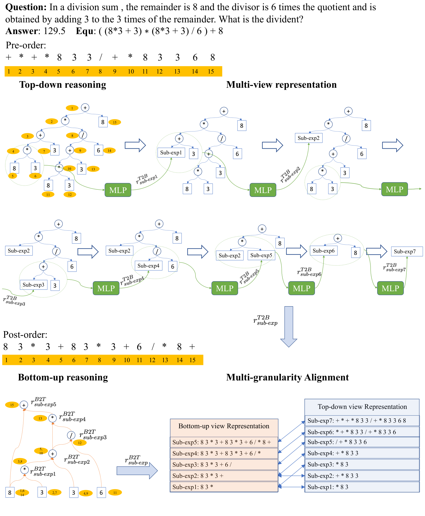
In Figure A2, we show an example from MathQA. The top-down process breaks down the overall problem through 15 reasoning procedures which are exactly the same as the pre-order traversal. Each reasoning step includes two steps: node prediction and node decomposition, until the leaf node (quantity nodes). Meanwhile, the bottom-up view predicts the entire equation after five relation extractions following the post-order equation. Two reasoning views work in reverse order.
Then, in the consistent contrastive learning process, the top-down view continuously computes the sub-expression representation based on the sub-tree fusion. For bottom-up reasoning, we directly use the embeddings from each relation extraction as representations. Since the bottom-up process reuses the previously constructed sub-expressions (step and ), it generates fewer sub-expressions than the top-down process. Finally, all sub-expressions representations from both views are aligned in the same latent space.
A.3 Case Study
We perform a case study to demonstrate the capability of generating diverse equations. As Figure A3 shows, the algorithm generates equivalent equations that are not the same as the labeled equations.
Most of these predicted equivalent equations can be derived from labeled equations by simple mathematical deformations, e.g., and in case 6. In addition to simple deformations, our algorithm also can solve complex problems using the different solving ideas, e.g., in case 8, it starts from a simpler reasoning idea and solves the problem correctly.
At the bottom of Figure A3, we also count the deformation pattern distributions among all diverse prediction equations. We summarize six patterns: addition and multiplication commutative law, multiplication and division distributive law, different problem-solving idea and others. Then we manually identify the deformation patterns of each equivalent equation predicted by ours. We discover that more than half of the equivalent equations () can be derived from additive or multiplicative commutative law deformations. Nearly 30% of the equivalent equations can be derived by deforming the distributive law and about 8% belong to the different solving ideas (e.g., cases 8 and 9). It shows that our multi-view method has mathematical reasoning capabilities and can be applied to solve complex mathematical problems.