Stochastic methods for slip prediction in a sheared granular systemPreprint: APS/123-QED
Abstract
We consider a sheared granular system experiencing intermittent dynamics of stick-slip type via discrete element simulations. The considered setup consists of a two-dimensional system of soft frictional particles sandwiched between solid walls, one of which is exposed to a shearing force. The slip events are detected using stochastic state space models applied to various measures describing the system. We show that the measures describing the forces between the particles provide earlier detection of an upcoming slip event than the measures based solely on the wall movement. By comparing the detection times obtained from the considered measures, we observe that a typical slip event starts with a local change in the force network. However, some local changes do not spread globally over the force network. For the changes that become global, we find a sharp critical value for their size. If the size of a global change exceeds the critical value, then it triggers a slip event; if it does not, then a much weaker micro-slip follows. Quantification of the changes in the force network is made possible by formulating clear and precise measures describing their static and dynamic properties.
I Introduction
Stick-slip dynamics is ubiquitous in granular and soft matter systems as well as in many other ones, see de Arcangelis et al. 2016; Falk and Langer 2011 for reviews. Understanding the intermittent stick-slip dynamics is of utmost importance because of the relevance to large-scale possibly cataclysmic events such as earthquakes. Therefore, there is a large body of research focusing on quantifying and explaining intermittency in a variety of systems, see Daub and Carlson 2010; Kawamura et al. 2012; de Arcangelis et al. 2016; Luding et al. 2021 for reviews. For obvious reasons, there is an active interest in identifying precursors to the slip events that lead to abrupt structural rearrangements of the systems, see Scuderi et al. 2016 for a recent example in the context of earthquakes. Extensive research considering acoustic precursors of intermittent dynamics in laboratory experiments can be found in Johnson et al. 2013 and references therein.
The attempts to identify precursors of slip events, fractures, and shear bands have a long history; for brevity here we discuss only recent developments. Several precursors are identified in various experimental systems Nerone et al. 2003; Aguirre et al. 2006; Scheller et al. 2006; Zaitsev, V. Yu. et al. 2008. These works report the existence of structural rearrangements of particles and point out that they become more prominent as a slip event approaches. Consistent results are also obtained in simulations Staron et al. 2002; Maloney and Lemaitre 2004; Pica Ciamarra et al. 2010; Welker and McNamara 2011; Denisov et al. 2016; Uhl et al. 2015; Denisov et al. 2017; Barés et al. 2017. However, despite a large amount of work concerned with identifying the precursors of slip events, we are not aware that they have been used for predictive purposes so far.
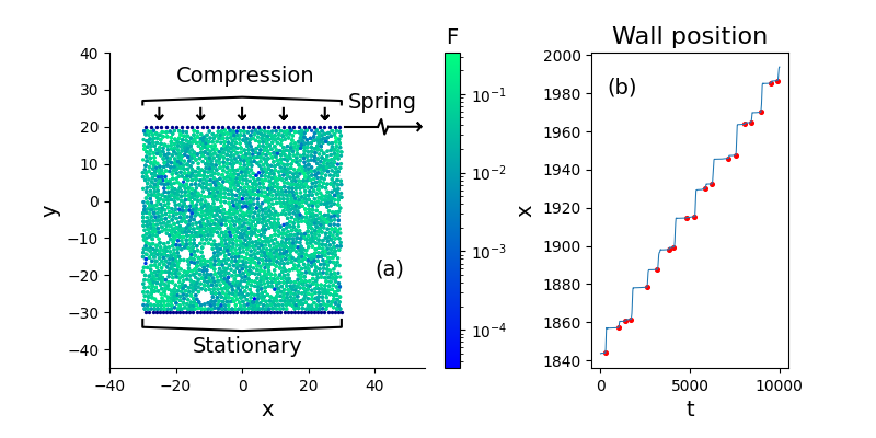
In our recent work Kramar et al. 2022, we considered a two dimensional system of soft disk-like particles simultaneously exposed to compression and shear, see Fig. 1(a). If the pressure is sufficiently large and the shearing speed is sufficiently small, then this system is found to exhibit intermittent dynamics of the stick-slip type Pica Ciamarra et al. 2010. By analyzing the outcome of discrete element simulations (DEMs), in Kramar et al. 2022 we demonstrate a fundamental difference between the measures defined as system-wide averages, and the measures that quantify the evolution of the system on a micro (particle) or mesoscale scale. The system-wide averages are found to be almost insensitive to an approaching slip, while the latter measures show a promising potential to serve as precursors of slip events, and will be considered in the present paper.
One significant obstacle in using the measures quantifying the evolution of the system on a micro or mesoscale scale for predicting an approaching slip event is that they are rather noisy and exhibit considerable variations between individual slip events. The method for delineating the slip events introduced in Kramar et al. 2022 is based on the wall velocity and requires the knowledge of the whole data set. Therefore, to identify the start of a slip event at time , the data for both and are used. We will refer to this method as the ‘offline method’ and note that such an approach, while logical and commonly used, is not suitable for predictive purposes.
In the present paper, we develop a method that can predict the slip events on-the-fly for an incoming stream of data. We will refer to this method as the ‘online method.’ The online method implemented in this paper is based on stochastic state space models (SSSMs) Petris et al. 2009 that are often used to model an observable signal by decomposing it into several dynamic components, such as trend (steadily increasing/decreasing part of the signal), seasonal (oscillations of the signal with different frequencies) or regressive components. Typically, these components are not directly observable but they can be modeled and used to predict the future values of the signal. SSSMs have been successfully used in meteorology Evensen 2009, robotics to guide autonomous vehicles Kwon and Park 2013, and track submarines Stone et al. 2014 as well as in economics Zhao et al. 2015; Shankar et al. 2012. A closely related application to our problem can be found in Wang et al. 2020 where the authors consider stochastic methods for modeling high-dimensional non-stationary spatio-temporal data collected at the sites with geological hazards. Another related application is the usage of machine learning to identify spatio-temporal clusters of surface displacement that are indicative of an imminent rock slide Das and Tordesillas 2019.
The applicability of SSSMs stems from the fact that the behavior of the considered measures is fundamentally different during the stick and slip regimes. The SSSMs allow us to predict the next value of a considered measure with good accuracy as long as the system is in the stick regime. The model is designed in such a way that it is too rigid to adapt to the evolution of the measure during the slip regime and its predictions become inaccurate when the system enters this regime. Thus, to detect the start of a slip event, we analyze the differences between the values predicted by the SSSM, and the observed values. In particular, we identify the start of a slip event as the time at which the error in our predictions becomes larger than a maximal acceptable value of the error, . As we will see, the online method based on SSSMs is rather general and can be in principle applied to any scalar measure that describes the evolution. Naturally, the upcoming slip event can be detected in advance only if the behavior of the considered measure changes before the slip event starts. For this reason, it is important to identify appropriate measures to consider. Here, we are guided by our previous work Kramar et al. 2022, which shows the predictive potential of the measures based on force networks. We will show in particular that the measures that are sensitive to local changes in the force network provide appropriate input to SSSMs.
One important part of the present paper is the investigation of how the detection time of the slip events depends on the considered measure and the value of . As the value of decreases, the upcoming slip events are detected earlier but the number of false positives increases. We will see that these false positives correspond to the so-called micro-slips which were reported in previous work on granular systems, see e.g. Dalton and Corcoran 2001; Johnson and Jia 2005; Johnson et al. 2007; Pica Ciamarra et al. 2010; Long et al. 2019, or local changes of the force network and possibly particle positions that do not lead to wall motion, see also Barés et al. 2017. By using SSSMs, we find that there is a clear separation between the slip events and micro-slips, similarly observed in previous works de Arcangelis et al. 2011; Long et al. 2019.
We also show that both slip events and micro-slip events are initiated by a local change of the force network, which first becomes global by spreading over the network, and only afterward does the shearing wall start moving. Some local changes dissipate instead of spreading and therefore do not lead to slip or micro-slip events. This connection between local and global changes and resulting wall activity has been discussed in the literature, see, e.g. Maloney and Lemaitre 2004; Dauchot et al. 2005; Barés et al. 2017; Stanifer and Manning 2022; however, the advancement in quantification of force networks and data analysis implemented in the present work now allows that connection to be explored for predictive purposes.
The rest of this paper is organized as follows. Section II.1 describes the simulated system, and the measures used for predictions are presented in Sec. II.2. In Sec. II.3 we introduce the framework for model-based slip detection. The general framework for stochastic models and the Kalman filter are reviewed in Sec II.3.2, while the models for the considered measures are specified in Sec. II.3.3. The main results are presented in Sec. III, followed by the conclusions in Sec. IV.
II Methods
II.1 Discrete element simulations
The simulations of dense granular material are carried out within a setup that leads to the stick-slip dynamics Kramar et al. 2022. The simulation techniques are identical to the ones described in detail in the previous work Kovalcinova et al. 2016 and here we provide just a summary. The material parameters used are motivated by experiments with photoelastic particles described e.g. in Dijksman et al. 2018. Figure 1 illustrates the simulated system and its behavior. The granular particles are modeled as 2D soft frictional disks. We place disks (system particles) between two horizontal rough walls placed parallel to the axis, see Fig. 1(a). The system particles are bi-disperse, with 25% of large particles and 75% of small particles with a size ratio of 1.25:1. The walls are constructed from small particles which are at a fixed distance from each other, see Kramar et al. 2022. The bottom wall is kept fixed, while the top one is pulled by a harmonic spring moving with the velocity in the direction.
The linear spring-dashpot model is used to describe the interactions between the system particles and between the system and wall particles. We use the diameter of small particles, , as the length scale, their mass, , as the mass scale, and the binary collision time, , as the time scale. Motivated by experiments Dijksman et al. 2018, we use cm, g, and s, as appropriate for particles of Young modulus of MPa. Then, the normal spring constant is N/m, and the tangential spring constant (needed for modeling of tangential forces using the Cundall-Strack model Cundall and Strack 1979) is taken as . The coefficient of static friction, , is equal to for particle-particle contacts and for particle-wall contacts (using a larger value here to reduce slipping of the system particles relative to the walls). The force constant of the spring applied to the top wall, , is significantly smaller than the one describing particle interactions, . The (constant) restitution coefficient is 0.5. In addition, a normal compression force is applied in the direction to model an externally applied pressure (force/length in 2D) of ; gravitational effects are not included. We note that with our choice of units, the numerical value of the applied pressure is of the same order of magnitude as the average overlap (compression) of the particles.
Stick-slip dynamics occurs for sufficiently large applied pressure and for sufficiently slow shearing, see, e.g. Pica Ciamarra et al. 2010. For we find by experimenting that the value leads to stick-slip. Then, we integrate Newton’s equations of motion for both the translation and rotational degrees of freedom using a fourth-order predictor-corrector method with time step . The states of the system, used to compute the quantities presented in this paper, are stored at times apart. In this paper, all the figures that show time-dependent results are in units of .
The simulations start by applying a pressure to the top wall and then letting the system relax until the ratio of kinetic/potential energy becomes sufficiently small Kramar et al. 2022. Then we start moving the spring in the direction, and, after the initial transient regime disappears, start collecting data. Figure 1(b) shows the horizontal position of the top wall for a short time window; the red dots illustrate the starts of slip events obtained using the offline method summarized in Sec. II.3.1. The complete simulation contains time output (first outputs are shown in Fig. 1(b)) and hundreds of slip events.
II.2 Measures
The analysis and detection of the slip events are based on three different measures whose potential was identified in Kramar et al. 2022. The first one, shown in Fig. 2(a), is the horizontal velocity, , of the top wall. The next measure is based on the properties of the differential force network; to define this network, we first discuss the concepts of the contact and force networks.

The contact network, , is a graph with one vertex at the center of each particle (excluding those in the top and bottom walls). There is an edge between two vertices of if the particles corresponding to these vertices are in contact at time . The force network is obtained by assigning weights to the edges in , representing the magnitudes of the normal force acting between the corresponding particles. A differential force network, , represents the differences between the force networks computed at two consecutive samples at and . Its edges are given by the union of the edges in the weighted graphs and . The weight on an edge in is the absolute value of the difference of the weights assigned to this edge in and if the edge is present in both. If the edge is not present in one of the force networks, we consider the corresponding weight in that force network to be zero. The measure that we use in what follows is the maximal force, , for which percolates between the left and right boundary of the domain (in Kramar et al. 2022 top-bottom percolation was considered as well, but we do not use that measure here for brevity).
The last measure quantifies the time evolution of the force network. For each force network, , we compute its persistence diagrams defined briefly here, and more fully in Zomorodian and Carlsson 2004; persistence diagrams were extensively used in our earlier works in the analysis of granular matter in various settings, see, e.g. Kramár et al. 2014a; Kramár et al. 2013; Kramár et al. 2014b. describes the structure of the supper-level sets of the force network . In particular, is a finite collection of points in such that . Every point in indicates that a connected component appears in the set consisting of the edges of with weights larger than and it merges with another connected component after adding all the edges with the weights larger than . To help interpretation, we note that the points in with coordinate sufficiently large (larger than the average force) describe the vague concept of ‘force chains.’ In the present work, for simplicity, we do not consider loops that could be described similarly by a separate , see Kramar et al. 2022 for more details.
The difference between two persistence diagrams can be measured by their Wasserstein distance defined precisely in Kramár et al. 2014a. This distance essentially sums up all the changes between the persistence diagrams in a manner analogous to the norm. In what follows, we encode the changes between the force networks and by considering the Wasserstein distance, between their persistence diagrams.
Figure 2 illustrates the measures described above. At the start of the slip events detected by the offline method, described in Sec. II.3.1, the value is still relatively close to its baseline typical for the stick regime. This is not the case for the other two measures. In particular, increases considerably before the detection time. We exploit this behavior to develop a new online method for detecting slip events that can produce an early warning before increases significantly.
II.3 Methods for detecting slip events
Figure 3 shows the stick-slip dynamics in more detail, with three illustrative examples of the behavior of the time series, (since there is no possibility of confusion, we drop the time dependence from now on). Even though the peaks of are well pronounced during the slip events, it is non-trivial to precisely define when individual events start. Difficulties in defining the start of a slip event arise from the oscillations of , visible in Fig. 3. In the considered system these oscillations are related to propagating elastic waves caused by the vertical () component of motion of the top wall, which is associated with each slip event Kramar et al. 2022.

Due to these complications, slip detection must be done carefully. One option is to employ an offline method, that uses the values of after the slip event has begun to distinguish it from oscillations; this approach was used in Kramar et al. 2022 and is outlined in Sec. II.3.1. Related methods were used in other works facing similar issues, see e.g. Long et al. 2019; Barés et al. 2017. An alternative is to use a more sophisticated online method that accounts for the oscillations. Stochastic state space models (SSSMs), discussed later in this section, provide a good framework for such an approach. To present the main idea, we use an example of . Note that the amplitude of the oscillations of can vary and tends to decrease as we approach the onset of a slip event. Therefore, during a stick can be modeled as a composition of several components. One component represents the level around which the oscillations occur, and several harmonic components with stochastically changing amplitudes reasonably reproduce the oscillations. To detect the start of a slip event based on , we exploit the fact that the behavior of this quantity is fundamentally different during the stick and slip regimes. So, the SSSM used to model the evolution during the stick regime does not provide good predictions if the system is not in this regime. This means that during slip events, the difference between the value predicted by the SSSM and the observed one becomes large. Thus, to identify the start of slip events we just need to detect when the difference between the predictions and observed values becomes sufficiently large.
Section III demonstrates that SSSMs can be used to devise an efficient online method for detecting the start of slip events. In particular, we will see that the algorithm tends to detect upcoming slip events earlier than the offline approach. This result opens the door for a real-time prediction of slip events. In what follows, we first review the offline approach in Sec. II.3.1, followed by a short background of stochastic models and Kalman filter in Sec. II.3.2.

II.3.1 Offline approach for detecting slip events
In the rest of this paper we will call slip events the events that are detected by this approach. To deal with the oscillations present in , shown in Fig. 3, the offline approach for detecting slip events Kramar et al. 2022 relies on a choice of two thresholds. The value of the first threshold, , is larger than the amplitude of the oscillations visible in the examples shown in Fig. 3, so the method avoids spurious detection of slip events. If exceeds , then a slip event is identified at time . However, at this time the wall has already begun to move with a non-negligible speed. For this reason, the offline method uses a second smaller threshold, , to find more precisely the start of each slip event. For this purpose, the algorithm moves back in time until the value of drops below . The time when this occurs is the starting point of the slip (the numerical values used for and are motivated in Kramar et al. 2022). The end of a slip event is identified as the time at which as well as its average over the next 50 outputs (roughly two periods of oscillations following a slip event) is smaller than . This algorithm is slightly different than the one detailed in Kramar et al. 2022, which uses the condition that the average over the preceding 50 outputs marks the end of a slip event. We make this change to avoid artificial termination of a slip event, which occurs when drops briefly below at the start of a slip event.
The main shortcoming of this approach (or any other approach based on using both past and future data for slip detection), is that it cannot be used for real-time detection of slip events. It detects the time at which the event starts only after the wall velocity exceeds the specified threshold. Moreover, the precise values of the thresholds influence the number and length of the detected events.
II.3.2 State Space Models and Kalman Filter

As discussed at the beginning of Sec. II.3, during the stick regime the signal specified by can be approximated by a composition of several components, one of them representing the level around which oscillations occur, and the rest describing oscillations. The behavior of the other measures is more complex. Figs. 4 and 5 show the and W2B0 measures during the same time windows as in Fig. 3. For example, to model W2B0, we have to account for both the oscillations and a decreasing trend of the signal.
We proceed by presenting the general idea behind stochastic modeling of a time series , which can be decomposed into several components whose characteristics are captured by the value of the state vector , which encodes the properties such as trend and oscillations of a considered measure. As commonly done in the literature Petris et al. 2009, we use a discrete time for the rest of this section, where is in units of , specified in Sec. II.1. For example, if represents the magnitude of the wall velocity, , then , the wall velocity at the physical time . To model the time series by a sequence of random variables we will use a special class of SSSMs known as dynamical linear models (DLMs). This choice is motivated by two independent factors. First, the necessary computations can be performed efficiently. Second, the models are sufficiently rich to properly capture the evolution of the considered measures during the stick regime while they are too rigid to assimilate the time evolution of these measures during the slip regime.
The main assumption of the DLMs is that the evolution of the -dimensional state vector, , is governed by a real Markov chain called the state process and the random variable is a noisy (imprecise) scalar observation of this chain. To be more precise, the evolution of is described by the equation
| (1) |
while the values can be reconstructed from via the equation
| (2) |
where and are known sequences of matrices of order and , respectively. Two independent sequences of random variables describing the observation error, and the model error, , are distributed according to zero mean normal distributions and , where the variances and covariance matrices are given. We will explain in Sec. II.3.3 how to specify , and for the measures considered in this paper. Here we just note that the models the evolution of the individual components of the signal and describes how to combine these components to obtain the random variable , which models the time series . The error (noise) terms are important because there might be external noise in the physical system and the relations described by are only approximate.
Unlike in deterministic systems, the value of is not known precisely. Instead, the probability that has a given value is expressed by a probability distribution , which in the case of DLMs is required to be a multivariate normal distribution. Given a DLM and the distribution , we can predict the value of as
| (3) |
where is the mean value of . The predicted value, , is known as the forecast and can be used to construct a prediction
| (4) |
of the next value of the modeled time series. In particular, if we know , then Eqs. (3) and (4) allow us to predict the value of . However, we usually do not know the initial distribution . The fact that is not known can be overcome by using the iterative procedure known as the Kalman filter Petris et al. 2009, which uses the Bayesian probability to improve our knowledge about the distribution of by incorporating the observed data . This is done by computing the conditional distribution . In practice, if the DLM is an appropriate model for the time series and the initial (prior) distribution is given by a normal distribution with large variance, then after a short burn-in period the conditional distribution describes the state with reasonable accuracy, and the model provides satisfactory predictions of the future states of the time series .
The precise definitions of and depend on the particular measure considered and will be provided in Sec. II.3.3. On the other hand, to quantify the observation error and model error we use standard universal methods. Here we only provide their brief summary; detailed exposition is available Petris et al. 2009. The shape of the covariance matrix for the model error is given by the discount factor method, i.e.,
| (5) |
where is the conditional covariance of and is the discount factor which will be specified for the individual measures in Sec. II.3.3. The value of corresponds to the overall accuracy with which describes the state update from to , referred to in Petris et al. 2009 as ‘model trust.’ Note that if , then Eq. (3) does not contain noise, and the evolution of is deterministic.
The variance of the observation error is modeled by a time-invariant unknown random variable, , estimated from the data at each time . To be compatible with the iterative scheme defined by the Kalman filter, the variable has to be inverse gamma distributed. For the initial (prior) distribution we choose the inverse gamma distribution . This is a ‘vague’ prior in the Bayesian terminology; it expresses a high degree of uncertainty as to the value of the unknown . By choosing a vague prior, the distribution of quickly responds to the data.
II.3.3 Specification of dynamical linear models (DLMs)
In this section we provide DLMs that model the evolution of the measures, defined in Sec. II.2, during the stick regime. To specify a DLM for a given measure we start by specifying the components of the state vector that capture the trend and oscillations of the signal. To describe the time evolution of the individual components of , given by the state process, Eq. (1), we need to set and the covariance matrix of the model error . We recall that is specified by choosing the discount factor . Finally, to forecast the value of the modeled measure, by using Eq. (2), we need to specify the observation function, , and the distribution of the observation error. As explained in Sec. II.3.2, the observation error is modeled by a time-invariant random variable estimated from the data at each time . The required initial distribution is always chosen to be the inverse gamma distribution .
Figures 3, 4, and 5 manifest that all considered measures exhibit oscillations, albeit with different frequencies. To model the oscillations we use a few harmonic components. For a given measure the frequency of the first harmonic component is set to its dominant frequency , determined by Fourier analysis of the first of the signal. The frequencies of the other harmonic components are natural multiples of . So, for each model, we specify the number of harmonic components and the discount factor .
Our extensive numerical investigation shows that all results discussed in Sec. III are robust under rather large variations of these two parameters. The final choice of the parameters for each model was guided by diagnostics of the normalized prediction error (NME) of the model defined as
| (6) |
where , is the transpose of the matrix and is the conditional covariance of . In other words, is a covariance of the conditional distribution of . If the model is a good fit for the data, then the NMEs are uncorrelated and they are distributed according to the standard normal distribution Petris et al. 2009. We use the Ljung-Box statistic to test Ljung and Box 1978 for possible autocorrelation and the Shapiro-Wilk test Shapiro and Wilk 1965 to see if the normalized errors are distributed according to the standard normal distribution. We chose the models that yield the best diagnostics during the stick regimes shown in Figs. 3, 4, and 5.
We start by setting up the model for the wall velocity, . Figure 3 shows that during the stick regime oscillates around an almost constant value. Note that oscillations exhibit multiple frequencies. Their dominant frequency was determined from the first of the data. These oscillations can be modeled satisfactorily with only two harmonic components with frequencies , for . The harmonic component with the frequency is represented by a pair of two variables that evolve in such a way that the point rotates around a circle with the constant frequency . Without the error (noise) terms, the radius of this circle would be constant as well. However, the error terms allow for a slow change of this radius.
The value around which the oscillations occur is represented by the last component of the state vector . The value of changes very slowly, and on the deterministic level we consider to be constant. We allow it to change only via the error term. The following equations, defining , formalize the described evolution of the components of
| (7a) | ||||
| (7b) | ||||
| (7c) | ||||
for . We note that both variables , for each value , oscillate with the same frequency and amplitude. Only their phase is different. To reconstruct the oscillations around the slowly changing value , it is sufficient to consider the variables for . The observation function, , just adds the individual components of the signal and is defined as
| (8) |
To specify the model error, , we use the discount factor . To initialize the DLM we need to define the initial (prior) distribution for the state . We use a normal distribution centered at mean where , for , , with the width specified by the scaled covariance matrix .
Now we turn our attention to the left-right percolation force, , shown in Fig. 4. The dominant frequency of oscillations for this measure is . Again it is sufficient to use two harmonic components with frequencies , . As in the case of , the evolution of the variables , representing the harmonic components, is described by Eqs. (7a) and (7b).
The most important difference between the behavior of and is that the value around which oscillates is not changing slowly. This value decreases in an approximately linear manner. To incorporate this decrease into the model, we need two state components: which models the slowly changing slope, and which captures the decreasing value around which the signal oscillates. These two components evolve according to the following equations
| (9a) | ||||
| (9b) | ||||
The observation function, , again sums the variables capturing the oscillations and the variable representing the value around which the oscillations occur, so . To specify the observation error we use the discount factor . As in the case of , the initial distribution for the state vector is a normal distribution centered at where , for , and the scaled covariance matrix .
The last considered measure, W2B0, exhibits oscillations with the dominant frequency , and using two harmonic components is once again sufficient. The most important difference between the behavior of and W2B0 is that the value around which W2B0 oscillates decays in a roughly exponential manner, see Figure 5. Thus, it can be modeled by a function where the value of is allowed to change slowly through the error term. To incorporate this exponential decrease in the model, we use two state components: which models the slowly changing value , and which captures the behavior of . The following equations ensure the desired evolution of these components
| (10a) | ||||
| (10b) | ||||
The discount factor is and the initial distribution for the state vector is a normal distribution centered at where , for , and the scaled covariance matrix .
Equation (10b) is non-linear, so the model is not a DLM and the Kalman filter cannot be used to compute the necessary conditional distributions. To accommodate the non-linearity of the function , we use the extended Kalman filter (EKF) Evensen 2009 which uses the Jacobian matrix of to compute the covariance of the predictive distribution of . There are well-known divergence problems with EKF Evensen 2009, since using the Jacobian matrix can lead to unrealistically small values of the covariance matrix of the state distribution. This can impede the ability of the filter to assimilate the observed data and eventually cause divergence of the model. In our case, this happens when the value of becomes too small and is rounded to zero. To retain numerical integrity during our computations, we re-initialize the filter upon encountering filter divergence. We note that this occurred only once in the entire data set.
III Results
Now we are ready to show how the dynamical linear models (DLMs) defined in Sec. II.3.3 can be used for the online detection of the slip events identified by the offline method. We will see that the DLMs detect not only the slip events but also additional events. The DLMs based on the wall velocity, , and the measure of the global change in the force network, , detect roughly the same events. However, the global changes of the force network are typically detected before the increased activity of the wall. The DLM based on W2B0, measuring local changes of the force network, identifies almost all events detected by the other two DLMs, and in addition, it detects extra events in which a local change of the force network appears but does not spread across the whole system. As expected, in events detected by both W2B0 and , the local changes of the force network are detected before the global changes.
III.1 Event detection by DLMs

By construction, the accuracy of the predicted values of a measure modeled by the DLM significantly deteriorates during the slip events detected by the offline method. To identify the events, during which the time evolution of a considered measure does not conform to the respective DLM, we choose a maximal acceptable value of the NME, . The events detectable by the DLM and a given error threshold, , are obtained as follows. The start of an event is considered to occur at time if the NME, , satisfies and . While one could define that the event ends when the value of drops below , it is possible that the value of becomes accidentally small during a slip event detected by the offline method. Therefore, to declare that the event ends at , we require that all the values are smaller than . The value of is chosen to be roughly one period of the dominant oscillations present during the stick regime (see, e.g., Fig. 3) corresponding to .
To illustrate the dependence of the starting time of a detected event on the value of , we proceed by considering an example of two events detectable by all DLMs. The first event, shown in Figs. 6(a)-(c), is a slip event detected by the offline method. In contrast, Figs. 6(d)-(f) show a micro-slip, which is not detected by the offline method. This nomenclature is motivated by the literature Dalton and Corcoran 2001; Johnson and Jia 2005; Johnson et al. 2007; Pica Ciamarra et al. 2010; Long et al. 2019, which also distinguishes slips and micro-slips. In the present work, micro-slips are events that are not detected by the offline method but are detected by the DLM based on for . This particular value of is motivated below. In what follows we will also see that there are events detectable only by the DLM based on W2B0. Any event detected by W2B0 for which cannot be detected by the DLM for is called a ‘local change’; this particular numerical value is motivated below.
Figures 6(a)-(c) compare detection times of a slip event obtained by DLMs of , , and W2B0, respectively, for three different values of . Clearly, decreasing the value of leads to an earlier detection time. We note that for each fixed value of , the DLM for W2B0 detects the event first, followed by , and then .
Figures 6(d)-(f) show a micro-slip event and illustrate some difficulties that may arise if a single threshold value, , is chosen. Namely, the DLM for does not detect this event for and , since the NME rises only slightly above . On the other hand, using for W2B0 does not lead to a transition detection inside the depicted time window. The start of the event is detected before the shown time window starts and the event lasts through the whole time window. Therefore, if is too large, then slip events may be detected late or even missed, while choosing too small may result in erroneously classifying parts of a stick regime as a slip, micro-slip, or local change event. For this reason, in what follows we will consider a range of values.

With this example in mind, we now examine the entire data set. Figure 7(a) plots the number of events detected by DLMs for the considered measures. We observe that each of the measures shows a prominent peak, located at for and , and for W2B0. If we decrease below (as specified for each of the measures), then distinct events start to merge and their number decreases. Eventually, as approaches zero, all the events merge into a single one. Thus, from now on we will only consider the values of . Note that earlier in this section, we used the value of () at which the largest number of events can be detected by (W2B0) to define micro-slip (local change) events.
As the value of increases, the number of detected events decreases. This is caused by the disappearance of events during which the NME does not exceed , see e.g., Fig. 6(d). Figure 7(a) shows that for and there is a pronounced plateau followed by a gentle rise. Further investigation shows that some events are followed by almost immediate aftershocks, see Fig. 3(b). Detection of these aftershocks causes this rise because, for small values of , the main event and its aftershock are identified as one event; however, as increases, both the main event and the aftershock are eventually identified as separate events. To avoid the identification of aftershocks as separate events and to accurately capture the number of distinct events, we consider an adjusted number of events, shown in Fig. 7(b). The aftershocks are removed by using the events detected at as a baseline. Different events detected at are counted as one if they occur during a single event detected at . The adjusted number of slip events decreases for all DLMs and values .
III.2 The insight provided by different measures
We continue by investigating the relation between the events detected by DLMs for different measures at . We say that two events detected by different measures are matched if the time intervals over which they take place overlap. By matching the events detected by , we find that of these events (slips and micro-slips) are also detected by . Moreover, () of the events detected by () are detected by W2B0. Hence, a disturbance of the wall, that causes the NME for to exceed , is typically accompanied by a local as well as global rearrangement of the force network detected by W2B0 and respectively.
On the other hand, () of the events detected by W2B0 at are not detected through (). Figure 8 shows an example of a local change event detected solely by W2B0. Figures 8(a)-(b) show that for and , the signal does not exhibit any strong deviation from the stick behavior modeled by the DLMs, and consequently their NMEs are small. However, the W2B0 signal significantly deviates from the predicted oscillatory behavior, see Fig. 8(c). The fact that there is no visible change in the quantifying the global changes of the network implies that the detected change of the force network is local. For this particular local change, we find that there is a large spike in the broken force, , defined as the sum of all (normal) forces at the contacts that are broken between time and the following output time, see Fig. 8(d). The spike in appearing at the same time as the spike in W2B0 indicates that, at least for this local change event, the change in W2B0 is strongly related to broken contacts. We note that similar local changes, including non-affine motion or rotations of the particles, have been discussed in previous works Maloney and Lemaitre 2004; Barés et al. 2017.

Now we turn our attention to the relation between the slip events detected by the offline method and events detected by the DLMs. At each , we match the events detected by the DLMs to the slip events. To better understand the composition of the matched events, we use two ratios: true positive rate and false positive rate. For a given DLM, the true positive rate, , is the ratio of the number of slip events that are detected by the DLM, and the total number of slip events. The false positive rate, , is the ratio of the events detected by the DLM that do not match any slip event, to the total number of events detected by the DLM. The large false positive rates are caused by the fact that the DLMs also detect micro-slip events and local change events which are not detected by the offline method. At this point, we cannot reliably predict which local change events will lead to a slip event. Further research will be necessary to address this issue.
Figure 9 depicts the ratios, and . Part (a) shows that for each DLM there is a range of values for which and thus each DLM is capable of detecting all slip events. For every DLM there is a considerable number of false positives at , see Fig. 9(b). Initially, decreases for all the measures but then it increases for both and (dashed lines). As before, this increase is caused by detecting the aftershocks as separate events, see Fig. 7. Thus, we also consider an adjusted in which the aftershocks are not included. Figure 9(b) shows that the adjusted is always decreasing and drops much faster than the non-adjusted .

To justify our earlier classification of the events detected by into slips and micro-slips we return to Fig. 7(b). The slope of the curve representing the adjusted number of events detected by changes the fastest around the value of (we call it the change point) where it crosses the dashed line representing the number of slip events detected by the offline method. This is indicative of the presence of two classes of events Mori and Kawamura 2006; de Arcangelis et al. 2011. Since at the change point the number of adjusted events is close to the number of slip events, and for becomes zero (therefore the micro-slip events completely disappear), the two classes mentioned above directly correspond to slip and micro-slip events. That is, the distinction between the two types of events is not artificial, but reflective of an inherent difference between them.
The same argument that we used for demonstrates that the events detected by also split into two classes roughly corresponding to slip and micro-slip events. This suggests that during slip and micro-slip events there is a close connection between the wall activity and the global rearrangements of the force network measured by . The W2B0 measure does not yield a separation of events into two obvious classes because the number of adjusted events detected by the DLM for W2B0, see Fig. 7(b), does not exhibit any clear change point. Thus, the connection between the wall activity and local changes of the force network, measured by W2B0, is much less obvious, since local changes may or may not lead to a slip or micro-slip event.

To further investigate the relation between wall movement and force network rearrangements, we introduce a different measure, , which is defined as the largest value of for which an event is still detectable. Figure 10 shows the relation between the values of obtained by different measures, with each point corresponding to an event detected by both measures specified on the axes labels.
For both slip and micro-slip events, Fig. 10(a) demonstrates a linear relation between the magnitudes by which the horizontal wall velocity () and the global change of the force network () deviate from the behavior expected in the stick regime. Note that the slope of the data points in this figure is different for the slip and micro-slip events. For the slip events, the wall speed increases more rapidly with . We note that if obtained by is larger than , then the event is almost certainly a slip event (see also Fig. 9(b)), while the events with are micro-slips. Thus, there is a relatively well-defined critical value for the ‘size’ of the global change of the force network, and surpassing this value leads to a slip event. Figure 10(b) indicates that determining whether a local change event will cause a slip event or not is more complicated. While very large (small) values of always correspond to a slip (micro-slip) event, there is a wide range of the values obtained by W2B0 for which we observe both slip and micro-slip events.
Next, we explore the relation between the value of and the wall displacement during a detected event. Figure 11(a) shows that the values of obtained by the measure are linearly proportional to the wall displacement. We also observe a relatively clear distinction between micro-slip and slip events, since the data in Fig. 11(b) shows a clear change of slope around the boundary between the slip and micro-slip events. This change further indicates that for the slip events the wall activity increases more rapidly with the growing global change in the force network, than for the micro-slips. Figure 11(c) relates the size of the local change of the force network and the wall displacement. Similarly to Figs. 10(b)-(c), there is a large range of values obtained by W2B0 for which both slip and micro-slip events can occur. A local change of the force network with in this range has uncertain consequences. It might dissipate without causing a global change in the force network or trigger a global change accompanied by a micro-slip or slip event. However, sufficiently small local changes never trigger a slip event while sufficiently large ones always do.

III.3 Predictive power of different measures
So far, we have compared the events detected by individual measures. It is also of interest to examine how early the slip events, identified by the offline method, can be detected by DLMs. Figures 6(a)-(c) suggest that the time at which the start of a slip event is detected by a DLM depends on both the considered measure and . To examine this quantitatively, we consider the times at which the offline method detects the start of the slip events as a baseline and compare them with the times obtained by different measures and values of . We emphasize that the purpose of this comparison is quantifying the effectiveness of the online methods based on DLMs, and not comparing the performance of online and offline methods. The offline approach uses future data for identifying slip events and is not appropriate for predictive purposes.
For a given slip event, let and be the times at which it is detected by the offline method, and by the DLM for the considered measure, respectively. We then define . If , then the slip event is identified in advance. To analyze how much in advance the slip events can be detected, using different measures and values of , we consider the median advance notice defined as follows. For a given measure and , the value is the median over all slip events detected by the DLM. Figure 12(a) shows this metric as a function of . We immediately observe that the measure tends to provide the earliest detection times for a wide range of ’s. In particular, for , the median advanced notice is over ten time units, while the best value that can be achieved by is only around five, and barely detects slip events in advance at all.

To obtain the portion of the slip events that are detected in advance, we divide their number by the number of all slip events. This fraction is denoted by . Figure 12(b) shows that , as expected, decreases with for each considered measure. Once again, the shape of the W2B0 curve is different from the other two. This curve decreases slower and is the only one that approaches unity as gets close to . Hence the detection method based on this measure is the only one that can predict almost all slip events in advance for .
Finally, we investigate how fast the wall moves at the start of the slip event detected by different measures. Figure 13 shows the median of at detection times as a function of . The median at each fixed value is taken over all slip events detectable by the given model and . As expected, all the curves are increasing with . Consistently with the results shown in Fig. 12, we find significantly lower values of when considering the W2B0 measure. That is, the detection based on the W2B0 measure takes place before the wall has begun to move appreciably.

IV Conclusions
In this work we present a method for detecting the onset of slip events that can be used on-the-fly for an incoming stream of data. The method is based on the fact that the behavior of the system during slip events is very different from the one during the stick regime. In particular, we consider three different measures describing the system: the wall velocity , maximum percolation force of the differential force network, , and the Wasserstein distance between the persistence diagrams quantifying the force networks, W2B0. For each of these measures, we build a dynamical linear model (DLM) capable of accurately predicting its behavior during the stick regime. However, the predictions provided by DLMs become inaccurate when the measures start to exhibit more complex behavior as the system approaches a slip event. Hence, to detect the upcoming slip event we analyze the differences between the predicted and observed values of these measures.
Our analysis based on shows a clear distinction between slip and micro-slip events. We find that global changes in the network measured by are essentially always associated with a slip or a micro-slip event that follows them. In particular, the measure provides a slightly earlier prediction of the upcoming slip events than . By using the W2B0 measure we identify local changes of the force network which might or might not spread over the force network and become global. We observe that only the local changes that become global are followed by a slip or micro-slip event. While micro-slips were reported in the previous works considering similar systems, see e.g. Uhl et al. 2015; de Arcangelis et al. 2011, and local changes (called ‘local avalanches’) were discussed recently as well Barés et al. 2017, we are not aware of such events being used for predictive purposes. From the predictive perspective, we note that the W2B0 measure shows the best performance, in terms of sensitivity. On the other hand, the high sensitivity of this measure also leads to a significant percentage of ‘false positives,’ in the form of local changes that do not lead to slip events.
In summary, we observe the following timeline of the changes leading to a slip event. Typical slip events start with a local change in the force network. The size of this local change can be quantified by the amount by which the observed values of W2B0 measure deviate from the predicted values. This deviation roughly corresponds to an increase in the W2B0 measure. If the size of the local change is sufficiently large, then it always becomes global and triggers a slip event. On the other hand, a sufficiently small local change does not trigger a slip event. There is, however, a large range of local change sizes for which the outcome is uncertain; the initial local disruption may either dissipate or trigger a global change resulting in a micro-slip or even slip event. While the chronology of a slip described above has been discussed in the literature already, our method allows for precise quantification of this timeline.
As noted above, a significant fraction of the local changes of the force network fall into an intermediary range and may or may not result in a slip or micro-slip event. It would be very much of interest to explore whether there are distinguishing characteristics of local changes that could be used to predict if the given change will lead to a slip event. In this work, we use W2B0 to identify local changes. This measure only compares the topological properties of the force network encoded by the persistence diagrams. Hence precise geometry of the force network is not considered. Further research will be necessary to establish if the geometry of the force and/or contact networks can be used to predict the outcome of local changes. Our results suggest that the use of stochastic state space models and in particular DLMs could be a productive path in this direction.
References
- de Arcangelis et al. (2016) L. de Arcangelis, C. Godano, J. R. Grasso, and E. Lippiello, Statistical physics approach to earthquake occurrence and forecasting, Phys. Reports 628, 1 (2016).
- Falk and Langer (2011) M. L. Falk and J. S. Langer, Deformation and failure of amorphous, solidlike materials, Annual Rev. Condens. Matter Phys. 2, 353 (2011).
- Daub and Carlson (2010) E. G. Daub and J. M. Carlson, Friction, Fracture, and Earthquakes, Annual Rev. Condens. Matter Phys. 1, 397 (2010).
- Kawamura et al. (2012) H. Kawamura, T. Hatano, N. Kato, S. Biswas, and B. Chakrabarti, Statistical physics of fracture, friction, and earthquakes, Rev. Mod. Phys. 84, 839 (2012).
- Luding et al. (2021) S. Luding, Y. Jiang, and M. Liu, Un-jamming due to energetic instability: statics to dynamics, Gran. Matt. 23, 1 (2021).
- Scuderi et al. (2016) M. M. Scuderi, C. Marone, E. Tinti, G. D. Stefano, and C. Collettini, Precursory changes in seismic velocity for the spectrum of earthquake failure modes, Nat. Geosci. 9, 695 (2016).
- Johnson et al. (2013) P. A. Johnson, B. Ferdowsi, B. M. Kaproth, M. Scuderi, M. Griffa, J. Carmeliet, R. A. Guyer, P.-Y. Le Bas, D. T. Trugman, and C. Marone, Acoustic emission and microslip precursors to stick-slip failure in sheared granular material, Geophys. Res. Lett. 40, 5627 (2013).
- Nerone et al. (2003) N. Nerone, M. Aguirre, A. Calvo, D. Bideau, and I. Ippolito, Instabilities in slowly driven granular packing, Phys. Rev. E 67, 011302 (2003).
- Aguirre et al. (2006) M. Aguirre, A. Calvo, I. Ippolito, A. Medus, and M. Mancuso, Rearrangements in a two-dimensional packing of disks, Phys. Rev. E 73, 041307 (2006).
- Scheller et al. (2006) T. Scheller, C. Huss, G. Lumay, N. Vandewalle, and S. Dorbolo, Precursors to avalanches in a granular monolayer, Phys. Rev. E 74, 031311 (2006).
- Zaitsev, V. Yu. et al. (2008) Zaitsev, V. Yu., Richard, P., Delannay, R., Tournat, V., and Gusev, V. E., Pre-avalanche structural rearrangements in the bulk of granular medium: Experimental evidence, Europhys. Lett. 83, 64003 (2008).
- Staron et al. (2002) L. Staron, J.-P. Vilotte, and F. Radjai, Preavalanche instabilities in a granular pile, Phys. Rev. Lett. 89, 204302 (2002).
- Maloney and Lemaitre (2004) C. Maloney and A. Lemaitre, Subextensive scaling in the athermal, quasistatic limit of amorphous matter in plastic shear flow, Phys. Rev. Lett. 93, 016001 (2004).
- Pica Ciamarra et al. (2010) M. Pica Ciamarra, E. Lippiello, C. Godano, and L. de Arcangelis, Unjamming dynamics: The micromechanics of a seismic fault model, Phys. Rev. Lett. 104, 238001 (2010).
- Welker and McNamara (2011) P. Welker and S. McNamara, Precursors of failure and weakening in a biaxial test, Gran. Matt. 13, 93 (2011).
- Denisov et al. (2016) D. Denisov, K. Lorincz, J. Uhl, K. A. Dahmen, and P. Schall, Universality of slip avalanches in flowing granular matter, Nat. Comm. 7, 10641 (2016).
- Uhl et al. (2015) J. T. Uhl, S. Pathak, D. Schorlemmer, X. Liu, R. Swinderman, B. A. W. Brinkman, M. LeBlanc, G. Tsenkenis, N. Friedman, R. Behringer, D. Denisov, P. Schall, X. Gu, W. J. Wright, T. Hufnagel, A. Jennins, J. Green, P. K. Liaw, T. Becker, G. Dresen, and K. A. Dahmen, Universal Quake Statistics: From Compressed Nanocrystals to Earthquakes, Nature Sci. Rep. 5, 16493 (2015).
- Denisov et al. (2017) D. V. Denisov, K. A. Lőrincz, W. J. Wright, T. C. Hufnagel, A. Nawano, X. Gu, J. T. Uhl, K. A. Dahmen, and P. Schall, Universal slip dynamics in metallic glasses and granular matter–linking frictional weakening with inertial effects, Sci. Rep. 7, 43376 (2017).
- Barés et al. (2017) J. Barés, D. Wang, D. Wang, T. Bertrand, C. S. O’Hern, and R. P. Behringer, Local and global avalanches in a two-dimensional sheared granular medium, Phys. Rev. E 96, 052902 (2017).
- Kramar et al. (2022) M. Kramar, R. Basak, C. Cheng, and L. Kondic, On intermittency in sheared granular systems, Soft Matt. 18 (2022).
- Petris et al. (2009) G. Petris, S. Petrone, and P. Campagnoli, Dynamic Linear Models with R (Springer, New York, NY, 2009).
- Evensen (2009) G. Evensen, Data Assimilation: The Ensemble Kalman Filter (Springer, New York, NY, 2009).
- Kwon and Park (2013) Y. Kwon and Y. Park, Improvement of vision guided robotic accuracy using kalman filter, Comput. Ind. Eng. 65 (2013).
- Stone et al. (2014) L. D. Stone, R. L. Streit, T. L. Corwin, and K. L. Bell, Bayesian Multiple Target Tracking (Artech House, Norwood, MA, 2014).
- Zhao et al. (2015) L. Zhao, X. Feng, and C. H. Meyer, Direct and accelerated parameter mapping using the unscented kalman filter, Magn. Reson. Med. 75 (2015).
- Shankar et al. (2012) R. Shankar, K. Chatterjee, and T. K. Chatterjee, A very short-term load forecasting using kalman filter for load frequency control with economic load dispatch, J. Eng. Sci. Technol. 5, 97 (2012).
- Wang et al. (2020) H. Wang, Q. Qian, and A. Tordesillas, Modeling big spatio-temporal geo-hazards data for forecasting by error-correction cointegration and dimension-reduction, Spat. Stat. 36 (2020).
- Das and Tordesillas (2019) S. Das and A. Tordesillas, Near real-time characterization of spatio-temporal precursory evolution of a rockslide from radar data: Integrating statistical and machine learning with dynamics of granular failure, Remote Sens. 11, 2777 (2019).
- Dalton and Corcoran (2001) F. Dalton and D. Corcoran, Self-organized criticality in a sheared granular stick-slip system, Phys. Rev. E 63, 061312 (2001).
- Johnson and Jia (2005) P. A. Johnson and X. Jia, Nonlinear dynamics, granular media and dynamic earthquake triggering, Nature 437, 871 (2005).
- Johnson et al. (2007) P. A. Johnson, H. Savage, M. Knuth, J. Gomberg, and C. Marone, Effects of acoustic waves on stick–slip in granular media and implications for earthquakes, Nature 451, 57 (2007).
- Long et al. (2019) A. A. Long, D. V. Denisov, P. Schall, T. C. Hufnagel, X. Gu, W. J. Wright, and K. A. Dahmen, From critical behavior to catastrophic runaways: comparing sheared granular materials with bulk metallic glasses, Gran. Matt. 21, 99 (2019).
- de Arcangelis et al. (2011) L. de Arcangelis, M. P. Ciamarra, E. Lippiello, and C. Godano, Micromechanics and statistics of slipping events in a granular seismic fault model, J. Phys.: Conf. Series 319, 012001 (2011).
- Dauchot et al. (2005) O. Dauchot, G. Marty, and G. Biroli, Phys. Rev. Lett. 95, 265701 (2005).
- Stanifer and Manning (2022) E. Stanifer and M. L. Manning, Avalanche dynamics in sheared athermal particle packings occurs via localized bursts predicted by unstable linear response, Soft Matter 18, 2394 (2022).
- Kovalcinova et al. (2016) L. Kovalcinova, A. Goullet, and L. Kondic, Scaling properties of force networks for compressed particulate systems, Phys. Rev. E 93, 042903 (2016).
- Dijksman et al. (2018) J. A. Dijksman, L. Kovalcinova, J. Ren, R. P. Behringer, M. Kramár, K. Mischaikow, and L. Kondic, Characterizing granular networks using topological metrics, Phys. Rev. E 97, 042903 (2018).
- Cundall and Strack (1979) P. A. Cundall and O. D. L. Strack, A discrete numerical model for granular assemblies, Géotechnique 29, 47 (1979).
- Zomorodian and Carlsson (2004) A. Zomorodian and G. Carlsson, Computing Persistent Homology (Springer, 2004).
- Kramár et al. (2014a) M. Kramár, A. Goullet, L. Kondic, and K. Mischaikow, Quantifying force networks in particulate systems, Physica D. 283, 37 (2014a).
- Kramár et al. (2013) M. Kramár, A. Goullet, L. Kondic, and K. Mischaikow, Persistence of force networks in compressed granular matter, Phys. Rev. E 87, 042207 (2013).
- Kramár et al. (2014b) M. Kramár, A. Goullet, L. Kondic, and K. Mischaikow, Evolution of force networks in dense particulate media, Phys. Rev. E 90, 052203 (2014b).
- Ljung and Box (1978) G. M. Ljung and G. E. P. Box, On a measure of lack of fit in time series models, Biometrika 65, 297 (1978).
- Shapiro and Wilk (1965) S. S. Shapiro and M. Wilk, An analysis of variance test for normality (complete samples), Biometrika 52, 591 (1965).
- Mori and Kawamura (2006) T. Mori and H. Kawamura, Simulation study of the one-dimensional burridge-knopoff model of earthquakes, J. Geophys. Res. Solid Earth 111 (2006).