Non-linear Electrodynamics in Blandford-Znajeck Energy Extraction

Maxwell’s electromagnetic theory (MED) is a widely used fundamental theory in both quantum physics and the context of cosmology. It is a well-known and recognized theory. In 1933 and 1934 Born and Infeld made the first attempts to change equations of MED Born 1933; Born and Infeld 1934 and tried to eliminate the divergence of the electron’s self-energy in classical electrodynamics. The Born-Infeld electrodynamics model does not contain any singularities because its electric field starts at its highest value at the center (which is equal to the nonlinearity parameter $b$), and then gradually decreases until it behaves like the electric field of Maxwell at longer distances. This model also ensures that the energy of a single point charge is limited. The parameter $b$ has a connection to the tension of strings in the theory Gibbons 2001; Fradkin and Tseytlin 1985, and there have been studies done to determine potential constraints for the value of $b$ in Davila et al. 2014; Ellis et al. 2017; Niau Akmansoy and Medeiros 2018; Niau Akmansoy and Medeiros 2019; Neves et al. 2021; Neves et al. 2022; De Fabritiis et al. 2022. In contrast to the Euler-Heisenberg electrodynamics Heisenberg and Euler 1936, the Born-Infeld model does not show vacuum birefringence when subjected to an external electric field. The Born-Infeld theory maintains both causality and unitarity principles. The Born-Infeld electrodynamics has served as inspiration for other models that are free of singularities and possess similar properties. For instance, various models presented by Kruglov in Kruglov 2007; Kruglov 2015a; Kruglov 2015b; Kruglov 2015c; Kruglov 2015d; Kruglov 2015e; Kruglov 2016a; Kruglov 2016b; Kruglov 2016c; Kruglov 2017a; Kruglov 2017b; Kruglov 2017c; Kruglov 2017c. Fang and Wang have presented a fruitful method for finding black hole solutions that have either electric or magnetic charges, in a theory that combines General Relativity with a nonlinear electrodynamics Fan and Wang 2016. Since then, numerous models have been advocated, and the effects of these theories—known as Non Linear Electrodynamics (NLED)—have been investigated in a wide range of contexts, not just those related to cosmology and astrophysics Mosquera Cuesta and Lambiase 2009a; Mosquera Cuesta and Lambiase 2011; Mosquera Cuesta and Lambiase 2009b; Corda and Mosquera Cuesta 2011; Mosquera Cuesta and Salim 2004a; Mosquera Cuesta and Salim 2004b; Mosquera Cuesta et al. 2006; Mbelek et al. 2007; Mbelek and Mosquera Cuesta 2008; Breton and Garcia-Salcedo 2007; Panotopoulos 2021; Panotopoulos and Rincón 2017; Toshmatov et al. 2018; Stuchlík and Schee 2019; Rayimbaev et al. 2022; Toshmatov et al. 2014; Abdujabbarov et al. 2016; Toshmatov et al. 2017; Stuchlík and Schee 2014, but also in non-linear optics Delphenich 2006, high power laser technologies and plasma physics Lundin et al. 2006; Lundstrom et al. 2006, nuclear physics Ohnishi and Yamamoto 2014; Akamatsu and Yamamoto 2013, and supeconductors Panotopoulos 2021. Many gravitational non-linear electrodynamics (G-NED), extensions of the Reissner-Nordstrom (RN) solutions of the Einstein- Maxwell field equations have gained a lot of attention (see Rincon et al. 2022; González et al. 2021; Rincón et al. 2018; Rincón et al. 2017; Diaz-alonso and Rubiera-Garcia 2013 and references therein). Additionally, Stuchlík and Schee have demonstrated that models that produce the weak-field limit of Maxwell are considered relevant, as opposed to those that do not provide the correct enlargement of black hole shadows in the absence of charges Stuchlík and Schee 2019. In particular, the existence of axially symmetric non-linear charged black holes (at least transiently) has been studied Mosquera Cuesta et al. 2017, indicating neutrinos as good probes thanks to their bountiful production in any astrophysical context. As a consequence, it would be interesting, in principle, to investigate the nature of electromagnetism (linear or not), due to different signatures in certain neutrino phenomena, such as neutrino oscillations, spin-flip and r-processes. The effect of non-linear phenomena on the BH shadow, BH thermodynamics, deflection angle of light and also wormholes have been investigated too Okyay and Övgün 2022; Övgün 2019; Kumaran and Övgün 2022; Pantig et al. 2022; Javed et al. 2022; Kuang et al. 2018; Javed et al. 2019; Javed et al. 2020; El Moumni et al. 2022; Uniyal et al. 2023; Jusufi et al. 2018; Halilsoy et al. 2014; Allahyari et al. 2020; Vagnozzi et al. 2022. In the context of primordial physics, instead, NLED, when coupled to a gravitational field, can give the necessary negative pressure and enhance cosmic inflation Garcia-Salcedo and Breton 2000 and some models also prevent cosmic singularity at the big bang Benaoum et al. 2022; Övgün 2017; Övgün et al. 2018; Otalora et al. 2018; Joseph and Övgün 2022 and ensure matter-antimatter asymmetry Benaoum and Ovgun 2021. The reason to consider NLED in the primordial Universe comes from the assumption that electromagnetic and gravitational fields were very strong during the evolution of the early universe, thereby leading to quantum correction and giving birth to NLED Kunze 2013; Durrer and Neronov 2013. Recently, the non-linear electrodynamics has been also invoked as an available framework for generating the primordial magnetic fields (PMFs) in the Universe Kunze 2008; Campanelli et al. 2008. The latter, indeed, is a still open problem of the modern cosmology, and although many mechanisms have been proposed, this issue is far to be solved. Seed of magnetic fields may arise in different contexts, e.g. string cosmology Gasperini et al. 1995a, inflationary models of the Universe Bamba et al. 2008; Turner and Widrow 1988, non-minimal electromagnetic-gravitational coupling Opher and Wichoski 1997; Bamba et al. 2010, gauge invariance breakdown Turner and Widrow 1988; Mazzitelli and Spedalieri 1995, density perturbations Matarrese et al. 2005, gravitational waves in the early Universe Tsagas et al. 2003, Lorentz violation Bertolami and Mota 1999, cosmological defects Vachaspati and Vilenkin 1991, electroweak anomaly Joyce and Shaposhnikov 1997, temporary electric charge non-conservation Dolgov and Silk 1993, trace anomaly Dolgov 1993, parity violation of the weak interactions Semikoz and Sokoloff 2004. The current state of art points to an unexplained physical mechanism that creates large-scale magnetic fields and seems to be present in all astrophysical contexts. They might be remnants of the early Universe that were amplified later in a pregalactic period, according to one idea. To create such large-scale fields, super-horizon correlations can only still be created during inflationary epochs. However, it is still unclear how the electromagnetic conformal symmetry is broken. Different theoretical techniques have been taken into consideration for this, most notably non-minimal coupling with gravity, which by its very nature broke conformal symmetry (Capozziello et al. 2022 and reference therein). In a minimal scenario, electromagnetic conformal invariance can also be overcome. In this instance, the major goal is to modify the electromagnetic Lagrangian to a non-linear function of $F\doteq(1/4)F_{\mu\nu}F^{\mu\nu}$, as done in Kunze 2008; Campanelli et al. 2008; Cuesta and Lambiase 2009.

Since all NLED models significantly depend on scale factors (dimensionless or not), which may cause overlaps with other physics observables, it is obvious that determining the presence of non-linear phenomena is not free of uncertainty. Energy extraction from black holes, which is connected to various significant astrophysical events, including black hole jets and therefore Gamma-ray bursts (GRBs), is one area where NLED effects have not yet been properly studied Komissarov 2005. The Blandford-Znajeck (BZ) process Blandford and Znajek 1977; Tchekhovskoy et al. 2010; Lee et al. 2000; Tchekhovskoy et al. 2008; Komissarov and Barkov 2009; Ruffini and Wilson 1975 and the (very recent) magnetic reconnection mechanism Comisso and Asenjo 2021; Carleo et al. 2022 are the two different energy extraction techniques used today, along with a revised version of the original Penrose process Wald 1974 called magnetic Penrose process Stuchlík et al. 2021; Tursunov et al. 2020; Dadhich 2012. Among them, the BZ mechanism is still the most widely accepted theory to explain high energy phenomena Sharma et al. 2021; Takahashi et al. 2021 (even if there are still open questions in certain models or combinations King and Pringle 2021; Komissarov 2021; Komissarov 2005). It involves a magnetic field generated by the accretion disk, whose field lines are accumulated during the accretion process and twisted inside the rotating ergosphere. Charged particles within the cylinder of twisted lines can be accelerated away from the black hole, composing the jets. A characteristic feature of this mechanism is that the energy loss rate decays exponentially. This has been confirmed in a good fraction of observations (X-ray light curves) of GRBs Contopoulos et al. 2017. Furthermore, black holes with brighter accretion disks have more powerful jets implying a correlation between the two. Even if accretion onto a black hole is the most efficient process for emitting energy from matter it is not able to reach the energy rate of the GRBs, while other energy extraction ways such as the Hawking radiation give predictions on temperature, time-scale and energy rate highly in conflict with the observations RUFFINI 2002. Numerical models of black hole accretion systems have significantly progressed our understanding of relativistic jets indicating two types of jets, one associated with the disc that is mass-loaded by disc material and the other associated directly with the black hole McKinney 2006. In the first case, however, jets with high Lorentz factors are not supported. The BZ process, which produces highly relativistic jets by electromagnetically extracting black hole spin energy, remains the most astrophysically plausible mechanism to do so and is in good agreement with direct observations Steiner et al. 2012. In this sense, understanding the general relativistic magnetohydrodynamic (GRMHD) model of the bulk flow dynamics near the black hole (where relativistic jets are formed) is essential to study the central engine.

In this paper, in order to determine if non-linear effects may change the rate of energy extraction and the magnetic field configuration surrounding a (non-charged) black hole encircled by its magnetosphere, we will investigate the Blandford-Znajek mechanism in the context of the NLED framework.

The layout of the paper is as follows: in Sec. II we derive, for the first time, the general version of energy flux up to second order in the spin parameter. Sec. III is devoted to computing and solving the magnetohydrodynamic problem in Kerr-Schild coordinates, searching, in particular, for separated (monopole and paraboloid) solutions. In Sec. IV we give some estimates of the energy extraction w.r.t. standard BZ mechanism. We study primordial magnetic fields from (minimally coupled) NLED for different non-linear models in Sec. V, while discussion and conclusions are drawn in the Sec. VI. In this work, we adopt natural units $G=c=1$ and for simplicity set $M=1$ in order to handle adimensional quantities ($r$,$a$,…). The negative metric signature $(+,-,-,-)$ is also adopted.

In this section, following Blandford and Znajek 1977 and McKinney and Gammie 2004, we derive the energy extraction rate for a spinning, non-charged black hole in presence of stationary, axisymmetric, force-free, magnetized plasma and an externally sourced magnetic field. In the Kerr-Schild coordinate ¹¹ 1 Unlike the classic Kerr coordinates, the Kerr-Schild ones ensure finiteness of the electromagnetic field on the horizon. Notice that here we use a different metric signature than McKinney and Gammie 2004 and that in Blandford and Znajek 1977 simpler Kerr coordinates are used., the axially symmetric spacetime line element is

	$\displaystyle ds^{2}$	$\displaystyle=$	$\displaystyle\Big(1-\dfrac{2r}{\Sigma}\Big)dt^{2}-\Big(\dfrac{4r}{\Sigma}\Big)drdt-\Big(1+\dfrac{2r}{\Sigma}\Big)dr^{2}-\Sigma d\theta^{2}-{\sin^{2}\theta}\Big[\Sigma+a^{2}\Big(1+\dfrac{2r}{\Sigma}\Big)\Big]d\phi^{2}$		(II.1)
		$\displaystyle+$	$\displaystyle\Big(\dfrac{4ar\sin^{2}\theta}{\Sigma}\Big)d\phi dt+2a\Big(1+\dfrac{2r}{\Sigma}\Big)\sin^{2}\theta d\phi dr,$

where $\Sigma:=r^{2}+a^{2}\cos^{2}\theta$, $\Delta=r^{2}-2r+a^{2}$. The metric determinant is $g:=|det(g_{\mu\nu})|=-\Sigma^{2}\sin^{2}\theta$. We consider now a general electromagnetic Lagrangian governing the surrounding plasma and call it ${L}_{NLED}$; it is generally a function of the two invariants $X:=(1/4)F_{\mu\nu}F^{\mu\nu}$ and $G:=(1/4)F_{\mu\nu}F^{*\mu\nu}$, where, called $A_{\mu}=(\Phi,-\mathbf{A})$ the four-potential, $F_{\mu\nu}=\partial_{\mu}A_{\nu}-\partial_{\nu}A_{\mu}$ is the electromagnetic field strength tensor and $F^{*\mu\nu}=\frac{1}{2}F_{\alpha\beta}\epsilon^{\alpha\beta\mu\nu}$ is its dual ($\epsilon$ is the anti-symmetric Levi-Civita tensor ). Clearly, Maxwell theory is recovered when ${L}_{NLED}=-X$. The energy-momentum tensor, in absence of magnetic charges, is

$$T_{\mu\nu}^{EM}:=\dfrac{2}{\sqrt{-g}}\dfrac{\delta L_{NLED}}{\delta g^{\mu\nu}}=-L(X)g_{\mu\nu}+L_{X}F_{\mu\rho}F_{\nu\sigma}g^{\rho\sigma},$$

(II.2)

where with $L_{X}$ we indicate the derivative of $L$ w.r.t. $X$. In principle, the total energy-momentum tensor should also take matter contribution into account, i.e. $T_{\mu\nu}^{tot}:=T_{\mu\nu}^{EM}+T_{\mu\nu}^{MAT}$, but in the free-force approximation the latter disappears McKinney and Gammie 2004. This leads to

$$\nabla^{\nu}T_{\mu\nu}^{tot}\approx\nabla^{\nu}T_{\mu\nu}^{EM}=0,$$

(II.3)

together with the generalized Maxwell equations

$$\dfrac{1}{\sqrt{-g}}\partial_{\mu}\Big[\sqrt{-g}L_{X}F^{\mu\nu}\Big]=-J^{\nu},$$

(II.4)

$$\partial_{\mu}F^{*\mu\nu}=0,$$

(II.5)

with $J^{\nu}=(\rho,\mathbf{J})$ the four-current density. Since the plasma is assumed ideal, the electric field in the particle frame, $\mathbf{E^{\prime}}$, is zero. However, the presence of an external magnetic field leads to a non-zero electric field $\mathbf{E}$, but the ideal MHD approximation implies that $\mathbf{E}\cdot\mathbf{B}=0$, i.e. $G=0$, from which McKinney and Gammie 2004

$$\dfrac{\partial_{\theta}A_{t}}{\partial_{\theta}A_{\phi}}=\dfrac{\partial_{r}A_{t}}{\partial_{r}A_{\phi}}=:w(r,\theta),$$

(II.6)

where we introduced the function $w(r,\theta)$. With this notation, the electromagnetic tensor is

$$F_{\mu\nu}=\sqrt{-g}\left(\begin{array}[]{cccc}0&wB_{\theta}&-wB_{r}&0\\ -wB_{\theta}&0&-B_{\phi}&B_{\theta}\\ wB_{r}&B_{\phi}&0&-B_{r}\\ 0&-B_{\theta}&B_{r}&0\end{array}\right)$$

(II.7)

which automatically satisfies (II.4). The radial energy and angular momentum flux, as measured by a stationary long-distance observer, are given by

$$F^{(r)}_{E}:=T^{r}_{t},\;\;\;\;\;\;F^{(r)}_{L}:=-T^{r}_{\phi}\;.$$

(II.8)

Therefore

$$F^{(r)}_{E}=-L_{X}\Big(F_{t\theta}F_{\theta\phi}g^{r\phi}+F_{t\theta}F_{\theta r}g^{rr}-F^{2}_{t\theta}g^{rt}\Big)g^{\theta\theta},$$

and hence

$$F^{(r)}_{E}=L_{X}\Big[2B_{r}^{2}wr\Big(w-\dfrac{a}{2r}\Big)+wB_{r}B_{\phi}\Delta\Big]\sin^{2}\theta,$$

(II.9)

while the angular momentum flux is $F_{L}^{(r)}=F_{E}^{(r)}/w$. On the horizon, $r_{+}:=1+\sqrt{1-a^{2}}$, Eq. (II.9) reads as

$$F_{E}(\theta):=-2L_{X}^{(r_{+})}B_{r}^{2}wr_{+}(\Omega_{H}-w)\sin^{2}\theta,$$

(II.10)

where $L_{X}^{(r_{+})}:=L_{X}(r_{+},\theta)$ and $\Omega_{H}:=a/(2r_{+})$ is the angular velocity of the horizon. Apart from the factor $L_{X}$, these relations are equal to the linear (Maxwell) case. However, although the change is minimal, the physical consequences could be decisive. Indeed, $F_{E}(\theta)>0$ not only if $0<w<\Omega_{H}$, but also if $L_{X}<0$ at the horizon. Moreover, since $L_{X}$ is a function of $X$, and ²² 2 $X=\dfrac{1}{2}\left(|\mathbf{B}|^{2}-|\mathbf{E}|^{2}\right)$

$$X=\dfrac{1}{2}\Big[B_{r}^{2}(1-w^{2})+B_{\theta}^{2}(1-w^{2})+B_{\phi}^{2}\Big],$$

(II.11)

the energy flux will depend not only on the radial magnetic field $B_{r}$, but in general also on the other two components, namely $B_{\theta}$ and $B_{\phi}$. The power extracted (energy rate) is

$$P^{NLED}:=\iint d\theta d\phi\sqrt{-g}F_{E}(\theta)=4\pi\int_{0}^{\pi/2}d\theta\sqrt{-g}F_{E}(\theta).$$

(II.12)

In order to evaluate $P^{NLED}$, we need to solve MHD equations and find the expressions for $B_{r}$, $B_{\theta}$ and $B_{\phi}$. This is not an easy task, being quite laborious already in the standard Maxwell theory. As a first approach, we can certainly proceed with a perturbative series expansion in powers of $a$, as originally done in Blandford and Znajek 1977. Since typically one assumes $w=\Omega/2$, then $F_{E}\propto a^{2}$ so a Schwarzschild solution (i.e. $a=0$) is fine to obtain an expression for $P^{NLED}$ good up to second order in the spin parameter. It is clear that such a relation would be accurate only in the regime $a\ll 1$.
Since we want to completely solve the magnetohydrodynamic equations, instead of Eq. (II.3), we use the (equivalent) set of equations $F_{\mu\nu}J^{\nu}=0$, coming from free-force approximation. Only two equations are independent, and they give

$$J_{r}=-\mu(r,\theta)B_{r},\;\;\;\;J_{\theta}=-\mu(r,\theta)B_{\theta},\;\;\;\;J_{\phi}=-\mu(r,\theta)B_{\phi}+J_{t}w$$

(II.13)

where we defined $\mu:=-J_{\theta}/B_{\theta}=-J_{r}/B_{r}$. The above equations are formally equivalent to those of Blandford and Znajek 1977 and seem not to depend a priori on the specific NLED model. However, when coupled to Maxwell equations, difference with the linear theory appears clear. Indeed, in order to find the explicit expression for $\mu$ and $J_{t}$, from Eqs. (II.4), we get the following set of equations:

$$\begin{array}[]{cccc}\partial_{r}\Big[\sin^{2}\theta L_{X}B_{\theta}\Big(\Delta wY+4r^{2}w-2ra\Big)\Big]+\partial_{\theta}\Big[\sin^{2}\theta L_{X}\Big(2rB_{\phi}-wB_{r}Y\Big)\Big]=-J_{t}\Sigma\sin\theta\\ \partial_{\theta}\Big[\sin^{2}\theta L_{X}(2rwB_{r}+\Delta B_{\phi}-aB_{r})\Big]=-J_{r}\Sigma\sin\theta\\ \partial_{r}\Big[\sin^{2}\theta L_{X}(2rwB_{r}+\Delta B_{\phi}-aB_{r})\Big]=J_{\theta}\Sigma\sin\theta\\ \partial_{r}\Big[\sin^{2}L_{X}\theta\Big(2rawB_{\theta}-a^{2}B_{\theta}+\dfrac{\Delta B_{\theta}}{\sin^{2}\theta}\Big)\Big]+\partial_{\theta}\Big[\sin^{2}\theta L_{X}\Big(aB_{\phi}-\dfrac{B_{r}}{\sin^{2}\theta}\Big)\Big]=-J_{\phi}\Sigma\sin\theta\;.\end{array}$$

(II.14)

Together with Eqs. (II.13) and in a very similar way to Blandford and Znajek 1977, they lead to ³³ 3 Notice that our definition for $B_{\phi}$ differs from that of Blandford and Znajek 1977 by a factor $\sqrt{-g}$ (as assumed in McKinney and Gammie 2004) and we use Kerr-Schild coordinates.

$$\mu=-\dfrac{d}{dA_{\phi}}\Big[\sin^{2}\theta L_{X}\Big(\Delta B_{\phi}+2rwB_{r}-aB_{r}\Big)\Big]$$

(II.15)

where the explicit dependence on $L_{X}$ is shown. We will call $B_{T}$ the expression in square brackets by analogy with Blandford and Znajek 1977, even if, in our notation and coordinates, it will be not properly the toroidal field.
By putting $J_{t}$ from Eq. (II.14) into Eq. (II.13) and by using Eq. (II.15), the important differential equation for $A_{\phi}$ is found:

$$\begin{array}[]{cccccc}B_{\phi}\dfrac{dB_{T}}{dA_{\phi}}=\dfrac{w}{\Sigma\sin\theta}\Bigg[\partial_{r}\Big(\sin^{2}\theta L_{X}B_{\theta}(\Delta wY+4r^{2}w-2ra)\Big)+\partial_{\theta}\Big(\sin^{2}\theta L_{X}(2rB_{\phi}-wB_{r}Y)\Big)\Bigg]\\ -\dfrac{1}{\Sigma\sin\theta}\partial_{r}\Big[\sin^{2}L_{X}\theta\Big(2rawB_{\theta}-a^{2}B_{\theta}+\dfrac{\Delta B_{\theta}}{\sin^{2}\theta}\Big)\Big]-\dfrac{1}{\Sigma\sin\theta}\partial_{r}\Big[\sin^{2}\theta L_{X}\Big(aB_{\phi}-\dfrac{B_{r}}{\sin^{2}\theta}\Big)\Big].\end{array}$$

(II.16)

Notice that $w$, $B_{r}$ and $B_{\theta}$ are functions (only) of $A_{\phi}$ by definition of $F_{\mu\nu}$, hence Eq. (II.15) implies $B_{\phi}$ is only a function of $A_{\phi}$. In summary, our first unknowns $(B_{r},B_{\theta},B_{\phi},w)$, after using the ideal approximation (II.6), Maxwell equations (II.4) and the free-force approximation, have been reduced to one, namely $A_{\phi}$. Eq. (II.16), for $L_{X}=-1$, is also known as ’stream equation’, and its solution $A_{\phi}$ is called ’stream function’ Ghosh 2000.

In this section, we solve Eq. (II.16) in the static limit ($a=0$). This will be sufficient to have an expression for the extracted power up to second order in $a$.
Following Blandford and Znajek 1977, we assume that for $a\ll 1$

$$A_{\phi}=A_{\phi}^{(0)}+a^{2}A_{\phi}^{(2)}+\mathcal{O}(a^{4})$$

(III.1)

$$B_{\phi}=aB_{\phi}^{(1)}+\mathcal{O}(a^{3})$$

(III.2)

$$w=aw_{\phi}^{(1)}+\mathcal{O}(a^{3})$$

(III.3)

while $B_{\phi}=w=0$ when $a=0$. The functions $B_{\phi}^{(1)}$, $w_{\phi}^{(1)}$ and $A_{\phi}^{(2)}$ are unknowns, while $A_{\phi}^{(0)}$ is just the solution for Schwarzschild case. The other components of $\mathbf{B}$ are

$$B_{r}=-\dfrac{1}{\sqrt{-g}}\Big(\partial_{\theta}A_{\phi}^{(0)}+a^{2}\partial_{\theta}A_{\phi}^{(2)}\Big)\;\;,$$

(III.4)

$$B_{\theta}=\dfrac{1}{\sqrt{-g}}\Big(\partial_{r}A_{\phi}^{(0)}+a^{2}\partial_{r}A_{\phi}^{(2)}\Big)$$

(III.5)

It is clear that, in the static limit, the only unknown function is $A^{(0)}_{\phi}$. Indeed, at zero order in $a$ ($\sim\mathcal{O}(1)$), Eq. (II.16) becomes

$$LA^{(0)}_{\phi}=0$$

(III.6)

where

$$L:=\dfrac{1}{\sin\theta}\dfrac{\partial}{\partial r}L_{X}^{(0)}\Big(1-\dfrac{2}{r}\Big)\dfrac{\partial}{\partial{r}}+\dfrac{1}{r^{2}}\dfrac{\partial}{\partial_{\theta}}\dfrac{L_{X}^{(0)}}{\sin\theta}\dfrac{\partial}{\partial{\theta}}$$

(III.7)

where $L_{X}^{(0)}$ is $L_{X}$ in the Schwarzschild limit ⁴⁴ 4 A solution for $A^{(2)}_{\phi}$ requires a second order equation. See appendix.. For a power-law model $L_{NLED}=-CX-\gamma X^{\delta}$ Cuesta and Lambiase 2009, for example, it would be ⁵⁵ 5 Generally, $L_{X}$ is an even function of $a$, i.e $L_{X}=L_{X}^{0}+a^{2}L_{X}^{2}+\mathcal{O}(a^{4})$. It is essential that $L_{X}^{0}\not=0$ in order to have a solution.

$$L_{X}^{(0)}=-C-\gamma\delta\Big(\dfrac{-1}{2r^{2}\sin\theta}\Big)^{\delta-1}\Big(\partial_{\theta}A^{(0)}_{\phi}\Big)^{2(\delta-1)}.$$

(III.8)

Let us now consider separated solutions for $A_{\phi}$ and also assume a similar form for $L_{X}$, i.e.

$$\begin{array}[]{ccc}A^{(0)}_{\phi}=R(r)\cdot U(\theta)\\ L_{X}^{(0)}=f(r)\cdot g(\theta).\end{array}$$

(III.9)

With this ansatz, Eq. (III.6) reads as

$$\dfrac{\partial}{\partial\theta}\left[\dfrac{g(\theta)}{\sin\theta}\dfrac{\partial U(\theta)}{\partial\theta}\right]=-K\dfrac{g(\theta)U(\theta)}{\sin\theta},$$

(III.10)

$$\dfrac{\partial}{\partial r}\left[f(r)\left(1-\dfrac{2}{r}\right)\dfrac{\partial R(r)}{\partial r}\right]=K\dfrac{R(r)f(r)}{r^{2}}$$

(III.11)

where $K$ is a separation constant. We will choose $K=0$ so as to obtain the simplest solution (the lowest order⁶⁶ 6 One in principle can generalize to higher orders as done, for example, in Ghosh 2000. one).
From here on, the specific NLED model must be chosen. Assuming a power-law model ⁷⁷ 7 The so-called Kruglov model Kruglov 2015a, for example, is not separable, while the Born-Infeld one reduces to a power-law. and hence Eq. (III.8), we have to set $C=0$, unless one assumes $L_{X}^{(0)}$ is a function of just one variable, i.e. $f(r)=1$ or $g(\theta)=1$, but this would exclude most of NLED models. As a check, when $\delta=1$, we obtain the known solution as given in Ghosh 2000; Tchekhovskoy et al. 2010. For $\delta=2$, the latitudinal part does not change, i.e.

$$U(\theta)=\alpha\cos\theta+\beta$$

(III.12)

while the radial part strongly changes

$$R(r)=c\left(6r^{5}+15r^{4}+40r^{3}+120r^{2}+480r+960\ln(r-2)-2192+d\right)^{1/3}$$

(III.13)

where $\alpha$, $\beta$, $c$ and $d$ are constants. Following Ghosh 2000, we note that it is impossible to have a monopole solution⁸⁸ 8 The logarithmic singularity, also present in the linear limit, simply means that solutions are valid in regions of space which exclude event horizon. by default, as there are no combinations of constants to eliminate the radial dependence in $A_{\phi}^{(0)}$ without canceling all $R(r)$; it follows from Eq. (III.5) that $B_{\theta}\not=0$ . A separable paraboloidal solution ($\alpha+\beta=0=d$) is instead possible:

$$A^{(0)}_{\phi}\sim\big(\cos\theta-1\big)\big(6r^{5}+15r^{4}+40r^{3}+120r^{2}+480r+960\ln(r-2)-2192\big)^{1/3}.$$

(III.14)

For $\delta=3$ and higher values, the angular part will be equal to Eq. (III.12), while the radial one will be consistent only if $r<2$, i.e. beyond the event horizon, so we discard them. Same epilogue if one chooses negative powers ($\delta<0$): no monopole solution would exist and paraboloidal one would be valid only for $r<r_{+}$. This could be an interesting point: monopole solutions are actually not physical, while paraboidal magnetic configurations can explain the collimation of the jets Komissarov 2001; Nathanail and Contopoulos 2014. It must be emphasized that the geometry of the magnetic lines depends on the distance and thickness of the accretion disk, the only structure capable of generating a magnetic field. Therefore, exact solutions would require boundary conditions (see Ghosh 2000 and references therein) and therefore specific astrophysical scenarios. Moreover, also numerical simulations could come to our aid as done in McKinney 2006; Tchekhovskoy et al. 2008; Komissarov 2005; Penna et al. 2013. An interesting point of difference of (III.14) w.r.t. the analogous Maxwell solution is the forward displacement of the flow inversion point ($r\simeq 2.35$ vs $r\simeq 2.31$), i.e. the point in which $A^{(0)}_{\phi}$ change sign (and hence $R(r)=0$). However, as shown in Fig. (1), the main difference with linear theory is the asymptotic behaviour ($r\gg 1$) of the solution, being $A^{(0)}_{\phi}\sim r^{s}(1-\cos\theta)$ with $s>1$ in the non-linear case ($s=1$ in linear theory). This stronger ’verticality’ could favor these kind of solutions in the formation of jets.

In this section, starting from the result of the previous section, we find an estimate of the extracted power comparing it with the linear theory (Maxwell) case. Here, we propose two different ways.
Given the presence of the singularity at $r=2$ we have to discard this point. In order to use Eq. (II.12), which is evaluated on the horizon, we assume the condition $B_{r}\gg B_{\phi}$, which is often used in simulations ⁹⁹ 9 A purely radial magnetic field (monopole), although not realistic, is still considered today being the simplest configuration to implement Komissarov 2001, both numerically and analytically. . From Eq. (II.12), we find for the power extracted in the Maxwell case¹⁰¹⁰ 10 The (separable) paraboloidal Schwarzschild solution in linear theory goes like $A^{(0)}_{\phi}\sim(\cos\theta-1)(r+2\ln(r-2))$ as reported in Ghosh 2000. $P$, at the second order

$$P\simeq\dfrac{4\pi}{3r}\Big[r+2\ln(r-2)\Big]^{2}\Omega_{H}^{2}$$

(IV.1)

where $r>2$. On the other hand, in power-law model (III.14), similar computations lead to

$$P^{NLED}\simeq\dfrac{4\pi}{3r^{5}}\Big(6r^{5}+15r^{4}+40r^{3}+120r^{2}+480r+960\ln(r-2)-2192\Big)^{4/3}\Omega_{H}^{2}$$

(IV.2)

where we used

$$L_{X}^{(r)}=-\dfrac{1}{r^{4}}\Big(6r^{5}+15r^{4}+40r^{3}+120r^{2}+480r+960\ln(r-2)-2192\Big)^{2/3}$$

(IV.3)

instead of $L_{X}^{(r_{+})}$. Apart from the radial field approximation $B_{r}\gg B_{\phi}$, the rate is quite accurate¹¹¹¹ 11 Expressions for $P$ and $P^{NLED}$ are at fault only for a constant depending on the field configuration (monopole, paraboloidal, etc.). We assume that they are of the same order in both cases, as it is plausible.; it has been plotted as function of $r$ in Fig. (2). From the latter, it is clear that in principle such a NLED model could really extract more energy than in the conventional case. However, it would not have a Maxwellian limit because we had to impose $C=0$ to achieve the analytical solution (III.14).
The above estimate necessarily requires the stream function, i.e. a solution of the (very involved) stream equation. Moreover, it required to force $C=0$ for the power-law model. We can overcome these issues in the following way. As before, let us assume a radial field in the form $B_{r}=B_{0}\sin\zeta$, where $B_{0}\sim\sqrt{\sigma_{0}}$ is the magnetic strength as given by plasma magnetization $\sigma_{0}$ ($\zeta$ is the angle between $\mathbf{B}$ and $\hat{\phi}$ at the equator). Unlike before, let us evaluate Eq. (II.12) on the horizon $r=r_{+}$. Just by assuming $B_{\theta}$ negligible, it is straightforward to obtain an expression for $P^{NLED}$ without solving the stream equation and accurate up to second order in the spin parameter. This means that such an estimate would be suitable also for non-separable NLED model, like the Kruglov one $L_{NLED}=-X\cdot(1+\beta X)^{-1}$ Kruglov 2015a. Since in this framework $B_{\phi}=B_{0}\cos\zeta$, the rate w.r.t. Maxwell case simply is

$$\dfrac{P^{NLED}}{P}=\dfrac{1}{\left[\frac{\beta}{2}B_{0}^{2}+1\right]^{2}}\;.$$

(IV.4)

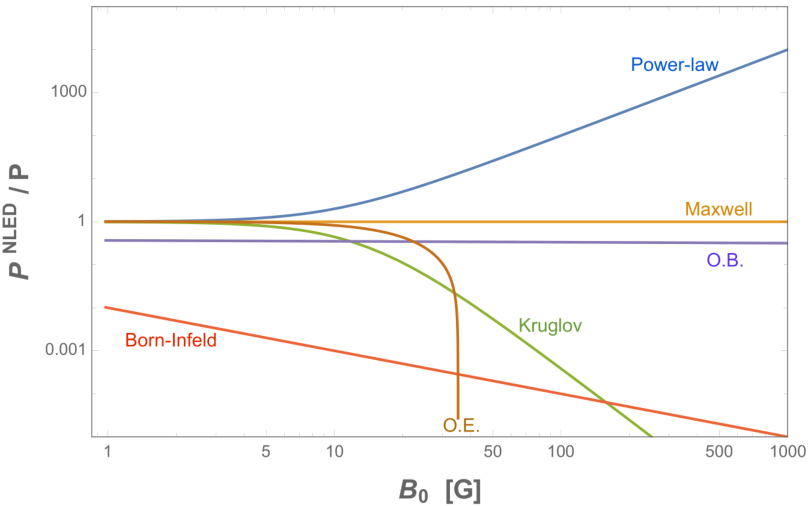
A similar computation was done for $L_{NLED}=-X-\gamma X^{2}$ and a comparison between these two different NLED models has been reported in Fig. (3). It is evident the advantage of power-law model with positive exponent ¹²¹² 12 A power-law electromagnetic model seems capable of extracting much more energy than models employing Kerr metric deformations. For example, in the case of a Johannsen metric, the extracted energy is no more than $\sim$10 times larger (Pei et al. 2016). In our framework, the ratio $P^{NLED}/P$ can exceed $10^{4}$ (see Fig. (3)).. In general, we have

$$\dfrac{P^{NLED}}{P}=-L_{X}(X_{0})$$

(IV.5)

where we defined $X_{0}:=B_{0}^{2}/2$. The strong dependence on the specific NLED model is clearly explicit: the ratio of energy power in presence of a non-linear electrodynamic model $P^{NLED}$ to linear (Maxwell) case $P$ is simply given by the opposite of the derivative of the lagrangian w.r.t. $X$ evaluated at $X_{0}:=B_{0}^{2}/2$. Notice that the two methods hold true in different regimes. While in the first way an assumption of type $B_{r}\gg B_{\phi}$ must be made, in the second estimate one needs $B_{\theta}\ll 1$. One can use one or the other depending on the specific context. From an astrophysical point of view, both observations and simulations suggest that the magnetic field around massive black holes has a poloidal configuration, i.e. the field lines lie in planes containing the axis of rotation Eatough et al. 2013; Liska et al. 2020; Event Horizon Telescope Collaboration 2021. Therefore, the assumption $B_{r}\gg B_{\phi}$ is physically achievable. About the second assumption, since a purely radial solution (monopole) is not likely, we generally expect $B_{\theta}\not=0$. However, except in extreme paraboidal cases, the polar component of the magnetic field is negligible for distances well beyond the event horizon (see Fig.(1) in Tchekhovskoy et al. 2010).

According to General Relativity (GR) primordial fields decayed adiabatically due to conservation of the flux. i.e. $a^{2}B\sim const$, and hence $B\sim 1/a^{2}$. Consequently, the magnetic energy density $\rho_{B}=|\mathbf{B}|^{2}/(8\pi)$ should have scaled as $1/a^{4}$, where $a$ is the scale factor of the (flat) Friedman-Robertson-Walker (FRW) metric. Since the scale factor diverges during inflation, this type of decay implies very faint magnetic fields at the end of the inflation period. This scaling is valid for every cosmic energy density present in the Universe, and then also for the cosmic microwave background (CMB), whose energy density (assumed almost constant during inflationary era) is given by $\rho_{\gamma}=\pi^{2}T^{4}/25$, or, in function of $a$, by $\rho_{\gamma}\sim 1/a^{4}$ (the extra factor $1/a$ w.r.t to matter, which decays as $\sim 1/a^{3}$, comes from energy redshift). Therefore, the ratio $r\doteq\rho_{B}/\rho_{\gamma}$ remained constant until today, with a current value of $r\approx 1$ and this constrain is a good tool to study primordial fields. The origin of large-scale magnetic fields has been studied not only in the context of GR but also in extended or alternative theories of gravity Kothari et al. 2020; Gasperini et al. 1995b; Atmjeet et al. 2014; Kothari et al. 2020. The main idea behind such works is to assume the non-conservation of the flux, breaking the conformal invariance of the electromagnetic sector and hence making possible a different trend from the adiabatic one for $\mathbf{B}$.
In this section, following Kunze 2008; Cuesta and Lambiase 2009; Capozziello et al. 2022 and in the context of GR, we try to find constrains on some NLED models, exploiting existence and survival of PMFs. We start from the action

$$S=\int d^{4}x\sqrt{-g}\dfrac{R}{2\kappa^{2}}+{L}_{NLED}$$

(V.1)

where $\kappa^{2}=8\pi$ and ${L}_{NLED}(X,G)$ encodes a general electromagnetic theory (see Sec. II). It is clear that Maxwell theory is obtained when ${L}_{NLED}=-X$. Varying the action w.r.t. the electromagnetic field $A_{\mu}$, the field equations are

$$\partial_{\mu}\Big[\sqrt{-g}\Big(L_{X}F^{\mu\nu}+L_{G}F^{*\mu\nu}\Big)\Big]=0$$

(V.2)

$$\partial_{\mu}F^{*\mu\nu}=0$$

(V.3)

which are the source free o zero density version of Eqs. (II.4)-(II.5). We consider here a conformally flat FRW metric

$$ds^{2}=a^{2}(\eta)\Big(d\eta^{2}-d\mathbf{x}^{2}\Big)=dt^{2}-a(t)d\mathbf{x}^{2}$$

(V.4)

where $\eta=\int_{0}^{t}a^{-1}(t)dt$ is the conformal time and $a(t)$ is a dimensionless scale factor. In this metric and with our signature, $F_{\mu\nu}$ can be written as

$$F_{\mu\nu}=a^{2}(\eta)\left(\begin{array}[]{cccc}0&E_{x}&E_{y}&E_{z}\\ -E_{x}&0&-B_{z}&B_{y}\\ -E_{y}&B_{z}&0&-B_{x}\\ -E_{z}&-B_{y}&B_{x}&0\end{array}\right)$$

(V.5)

in order to separate highlight the electric and magnetic fields as measured by a comoving (inertial) observer. With this ansatz and assuming the non-existence of magnetic charge, Eq. (V.2) becomes

$$A_{j}^{\prime\prime}+\dfrac{L_{X}^{\prime}}{L_{X}}A_{j}^{\prime}-\dfrac{\partial_{i}L_{X}}{L_{X}}(\partial_{i}A_{j}-\partial_{j}A_{i})-\Delta A_{j}=0$$

(V.6)

where $j=1,2,3$, $\Delta=:=\delta^{ki}\partial_{k}\partial_{i}$ and a prime denotes derivative w.r.t. conformal time. The above equation can be also written in terms of the electric $E_{j}$ and magnetic $B_{j}$ fields as

$$\partial_{0}\Big(a^{2}L_{X}\mathbf{E}\Big)-a^{2}\nabla\Big(L_{X}\mathbf{B}\Big)=0.$$

(V.7)

The zero component of Eq. (V.2) reads as

$$\nabla\Big(L_{X}\mathbf{E}\Big)=0$$

(V.8)

while the Bianchi identity gives

$$\partial_{0}\Big(a^{2}\mathbf{B}\Big)+a^{2}\nabla\times\mathbf{E}=0$$

(V.9)

as well as the usual constrain $\nabla\cdot\mathbf{B}=0$. Combining Eq. (V.7) and Eq. (V.9) one obtains

$$L_{X}F^{\prime\prime}+\Big(\partial_{0}L_{X}\Big)F^{\prime}=0$$

(V.10)

where we defined $F:=a^{2}B$ with $B:=|\mathbf{B}|$ and assumed the long-wavelength approximation Cuesta and Lambiase 2009 (i.e. disregarding spatial derivatives). Notice that in this approximation $F=F(\eta)$. By choosing a power-law model $L_{NLED}=-CX-\gamma X^{\delta}$, we recover the same results of Cuesta and Lambiase 2009. Here, we focus on other non-linear Lagrangian. As a first model, we consider Benaoum et al. 2022

$$L_{NLED}(X)=-\dfrac{X}{(\beta X^{\alpha}+1)^{1/\alpha}}$$

(V.11)

where $\alpha$ and $\beta$ are two real parameters with $\beta$ controlling the non-linearity contributions. A suitable condition for obtaining an analytical solution is the strong regime $(2a^{4}/F^{2})^{\alpha}\ll\beta$, i.e. $B\gg B_{0}$ with $B_{0}:=\dfrac{\sqrt{2}}{\beta^{1/(2\alpha)}}$, it follows from Eq. (V.10)

$$\dfrac{d^{2}F}{da^{2}}+\Bigg[\dfrac{s-1}{as}-4\dfrac{(\alpha+1)}{a}\Bigg]\dfrac{dF}{da}+8\dfrac{(\alpha+1)}{a^{2}}F^{2}=0$$

(V.12)

where $s={-1,2,1}$ depending on which primordial phase we are considering, i.e. inflation, reheating, radiation ¹³¹³ 13 We are assuming a scale factor of the type $a(\eta)=c_{s}\eta^{s}$, where $c_{s}$ is the Hubble constant for the specific primordial era. Notice that the values of $s$ are those of General Relativity; changing the gravitational sector in the action (V.1) leads to different $s$ values. See for example Capozziello et al. 2022. This is the only point in which, in a minimal approach, gravity comes into play.. Assuming a power-law solution for $F$, $F\sim a^{p}$, the inflationary exponent is

$$p_{\pm}=\dfrac{1}{2}\Big[3+4\alpha\pm\sqrt{\Sigma}\Big]$$

(V.13)

where we defined $\Sigma:=16\alpha^{2}-8\alpha-23$. This solution clearly constrains the parameter $\alpha$ to be either $\alpha>\frac{1}{4}(1+2\sqrt{6})$ or $\alpha<\frac{1}{4}(1-2\sqrt{6})$. When $\alpha=\frac{1}{4}(1\pm 2\sqrt{6})$ a pseudo-power-law solution is possible, namely

$$F(a)=c_{1}a^{p}-c_{2}a^{p}\ln{a}(3+4\alpha)$$

(V.14)

with $p=3/2+2\alpha$.
In the reheating epoch, the power-law solution $F\sim a^{q}$ reads as

$$q_{\pm}=\dfrac{1}{2}\Big[\frac{1}{2}+4(1+\alpha)\pm\sqrt{\Sigma}\Big]$$

(V.15)

with $\Sigma:=16\alpha^{2}+4\alpha-47/4$ and is valid when $\alpha<\frac{1}{8}(-1-4\sqrt{3})$ or $\alpha>\frac{1}{8}(-1+4\sqrt{6})$, while a pseudo-power-law solution for the remaining cases has $q=1/4+2(1+\alpha)$. With this solutions, it is possible to express the strong regime assumption in terms of conformal time, i.e. $\eta\gg\eta^{*}$ with $\eta^{*}$

$$\eta^{*}:=\Big[\dfrac{\sqrt{2}}{c_{s}^{\lambda-2}}\dfrac{1}{\beta^{1/2\alpha}F}\Big]^{\dfrac{1}{s(\lambda-2)}}$$

(V.16)

where $\lambda=\{p,p_{\pm},q,q_{\pm}\}$ and $c_{s}$ is the Hubble constant. Following Cuesta and Lambiase 2009, we can try now to constrain the only present parameter $\alpha$ exploiting the astrophysical observation $r\simeq 1$. Specifically, we found that this is possible only with the combination $(p_{-},q_{+})$, as shown, for different primordial conditions, in Table 1. Using these estimations, one can obtain a complete solution for the remaining radiation epoch. For example, taking $\alpha\simeq 15$, the power-law solution for the radiation era goes like $F\sim a^{u}$ with $u\simeq\{2,63\}$.

Similarly to what happens for the Born-Infeld model ¹⁴¹⁴ 14 A Born-Infeld model Born and Infeld 1934; Born 1933, does not allow either pseudo-power-law or power-law solutions. Expanding the Lagrangian in powers of $X$, however, leads to a power-law model with $\delta=2$ studied in Cuesta and Lambiase 2009, and hence to the same solutions, which, however, seems to exclude power-law Lagrangian $L_{NLED}=-CX-\gamma X^{\delta}$ with $\delta>2$. , also the exponential model Övgün et al. 2018

$$L_{NLED}=-\dfrac{Xe^{-\alpha X}}{\alpha X+\beta}$$

(V.17)

does not allow power-law solutions for $F$. Indeed, in this case, Eq. (V.10) becomes ($\alpha X\gg\beta$)

$$\dfrac{d^{2}F}{da^{2}}+\Bigg[\dfrac{s-1}{as}-2\dfrac{\alpha F^{2}}{a^{5}}\Bigg]\dfrac{dF}{da}+4\dfrac{\alpha F^{3}}{a^{6}}=0.$$

(V.18)

Alternatively, after expanding, the above model reduces to a power-law one with $\delta=2$ ($C=1/\beta$ and $\gamma=-\alpha/\beta$) as long as $\beta\leq 1$ and $B\ll\sqrt{2/\alpha}$. As for the Born-Infeld model and based on the results of Cuesta and Lambiase 2009, such a model is not compatible with the observation $r\sim 1$.
Concluding, while for the model (V.11) an analytical solution is available and an estimate of the parameter $\alpha$ is possible, the exponential one (V.17), at least in the regimes studied to have an analytical solution, is excluded from the observations, in a context of primordial magnetic fields.

In the literature, there are no known exact solutions for the magnetosphere of a spinning BH. In this paper, we analytically solved the maghehydrodynamic problem in the context of non-linear electrodynamics (NLED) models, trying to keep an approach as much model-independent as possible. We explored the Blandford-Znajek mechanism in the light of this framework in order to establish if non-linear effects can modify the energy extraction rate and the magnetic field configuration around a (non-charged) black hole surrounded by its magnetosphere. This attempt goes in the opposite direction to what was done in Konoplya et al. 2021, where the electromagnetic sector was unaffected, but a deviation from the familiar Kerr metric was switched on. Unlike Konoplya et al. 2021, in our work the black hole spin frequency $\Omega_{H}$ does not undergo changes, but, on the other hand, the formula for the extracted power deviates (not only numerically but also formally) from conventional one, i.e. with Kerr geometry and Maxwell theory. In particular, we found that the energy flux will depend not only on the radial magnetic field $B_{r}$, but in general also on the other two components, namely $B_{\theta}$ and $B_{\phi}$ and that, after perturbative expansion in powers of $a$ (as done in Blandford and Znajek 1977), no monopole solutions exist for power-law models $L_{NLED}=-CX-\gamma X^{\delta}$ and that only the case $\delta=2$ is significant. Paraboloidal solutions, instead, seems to be possible, and they strongly change if compared to linear theory case, especially in the radial part, as shown in Fig. (1). An interesting point of difference is the forward displacement of the flow inversion point ($r\simeq 2.35$ vs $r\simeq 2.31$), i.e. the point in which $A^{(0)}_{\phi}$ change sign (and hence $R(r)=0$). However, as shown in Fig. (1), the main difference with linear theory is the asymptotic behaviour ($r\gg 1$) of the solution, being $A^{(0)}_{\phi}\sim r^{s}(1-\cos\theta)$ with $s>1$ in the non-linear case ($s=1$ in linear theory). The more pronounced ’verticality’ could favor these kinds of solutions in the formation of jets, even if we do not explored the astrophysical consequences.
We also tried to derive several estimates for the extracted power. We used two different approaches valid in different magnetic regimes ($B_{r}\gg B_{\phi}$ or $B_{\theta}\ll 1$): one requiring the solution of the stream equation and one assuming the magnetic field strength as independent variable (see Figs. (2) and (3) respectively). In both cases, it appears evident that NLED power-law model with positive power can in principle extract much more energy w.r.t. classical Maxwell theory, and that, on the other hand, models like the Kruglov’s, for example, perform no better than the standard EM theory already does, making them rather unlikely. Even if separated solutions are not the only option, separable paraboloidal solutions seem to be in good agreement with numerical simulations even for rotating black holes, as rotation does not dramatically effects the magnestosphere configuration in this case Ghosh 2000. We notice that solutions have been found in the static limit ($a=0$) and that the expression for the extracted power are up to second order in $a$. Moreover, it would be interesting to investigate on higher order solutions ($K\not=0$) as done in Sec. 3 of Ghosh 2000, as well as on non-separable ones. Notice also that exact solutions would require boundary conditions (see Ghosh 2000 and references therein), therefore only numerical simulations (as done in McKinney 2006; Tchekhovskoy et al. 2008; Komissarov 2005; Penna et al. 2013) could be astrophysically meaningful. All these observations could be starting points for other works.
Finally, following Kunze 2008; Cuesta and Lambiase 2009; Capozziello et al. 2022, we tried to find constrains on some NLED models, exploiting existence and survival of PMFs. We focused on two recent NLED models, namely (V.11) and (V.17). After solving Maxwell equations, we found the constrain $\alpha\simeq 15$ for the first model, while the second model seems to be incompatible with the observation $r\sim 1$ (see Sec. I), at least in the regime we studied. In conclusion, our (analytical) results emphasize that the existence and the behavior of non-linear electromagnetic phenomena strongly depend on the model and the physical context, and that power-law models $L_{NLED}=-CX-\gamma X^{\delta}$ with $\delta\leq 2$ should be further studied.