AUC-based Selective Classification
Andrea Pugnana Salvatore Ruggieri
Scuola Normale Superiore University of Pisa
Abstract
Selective classification (or classification with a reject option) pairs a classifier with a selection function to determine whether or not a prediction should be accepted. This framework trades off coverage (probability of accepting a prediction) with predictive performance, typically measured by distributive loss functions. In many application scenarios, such as credit scoring, performance is instead measured by ranking metrics, such as the Area Under the ROC Curve (AUC). We propose a model-agnostic approach to associate a selection function to a given probabilistic binary classifier. The approach is specifically targeted at optimizing the AUC. We provide both theoretical justifications and a novel algorithm, called AUCROSS, to achieve such a goal. Experiments show that our method succeeds in trading-off coverage for AUC, improving over existing selective classification methods targeted at optimizing accuracy.
1 INTRODUCTION
The predictive performance of a classifier is typically not homogeneous over the data distribution. Identifying sub-populations with low performance is helpful, e.g. for debugging and monitoring purposes. In many socially sensitive application scenarios, we can consider not predicting at all for these sub-populations as an alternative to poor or even harmful predictions. Such applications include credit scoring, curriculum screening, access to public benefits, and medical diagnoses. Selective classification (or classification with a reject option) (Chow, 1970; Pietraszek, 2005) pairs a classifier with a selection function to determine whether a prediction should be accepted or the classifier should abstain. The selection function assesses the trustworthiness of a prediction. The literature on selective classification has mainly considered distributive loss functions. However, in many real-world scenarios, such as credit scoring (Engelmann, 2011), the quality of a binary probabilistic classifier is concerned with the discriminative power of the ranking induced by its scores (Huang and Ling, 2005). This is measured by the Area Under the ROC Curve (AUC) (Fawcett, 2006a) or, equivalently, by the Gini coefficient (Wu and Lee, 2014). Algorithms designed to minimize, e.g., the error rate may not lead to the best possible AUC values (Cortes and Mohri, 2003).
In this paper, we first introduce the problem of AUC-based selective classification, which consists of inducing a selective classifier which optimizes the AUC over the sub-population of accepted predictions while guaranteeing a minimum probability mass (called coverage) of such sub-population. We then focus on an instance of the AUC-selective classification problem, where we assume that: (i) the classification algorithm is given, including its hyper-parameters, and (ii) the selection function abstains on a range of the scores (score-based selective functions). Assumption (i) allows lifting an existing classifier to a selective classifier. In this respect, our approach is model-agnostic, as we do not make assumptions about the classification algorithm. Assumption (ii) is widespread in selective classification, supported by theoretical results (El-Yaniv and Wiener, 2010). Such an assumption allows for a theoretical analysis of the AUC-based selective classification problem. We devise AUCross, a model-agnostic algorithm for estimating the bounds of score-based selective functions that maximize the AUC for target coverage. The approach is based on a cross-fitting strategy over the training set. Bound estimates are supported by a theoretical analysis of (sufficient) conditions for abstaining that lead to an increase in the AUC. Experiments show that the approach performs very close to an oracle score-based selective function (which has access to the true class of instances), and it outperforms existing selective classification approaches targeted at optimizing accuracy.
The paper is organized as follows. Section 2 briefly surveys related work. Section 3 recalls basic concepts of selective classification and it introduces the AUC-based selective classification problem. Our theoretical approach is presented in Section 4, while we introduce AUCross algorithm in Section 5. Section 6 reports experimental results. Finally, we draw conclusions and outline possible extensions.
2 RELATED WORK
The two main models of selective classification are the cost model (Chow, 1970) and the the bounded-improvement model (Pietraszek, 2005). In the former, the goal is to minimize the expected cost, assuming a cost for misclassification and a cost for abstention, or a more refined cost based on the confusion matrix (Tortorella, 2005). In the Bayes optimal selective classifier, the selection function abstains when the posterior probability of the predicted class is below some threshold. Posterior probabilities can be estimated on a validation set by the plug-in rule (Herbei and Wegkamp, 2006). In the bounded-improvement model, the selection function is evaluated based on the probability mass of the accepted region (coverage) and the expected loss over such a region (selective risk). One can maximize coverage for a maximum target risk or minimize risk for a minimum target coverage (Geifman and El-Yaniv, 2017). Franc and Průša, 2019 establish the equivalence of cost-based and bounded-improvement models.
Most approaches for selective classification are model-specific in that they build the classifier and the selection function concurrently. Examples include methods for Support Vector Machines (SVM) (Fumera and Roli, 2002), boosted decision trees (Cortes et al., 2016), Deep Neural Networks (DNNs) (Geifman and El-Yaniv, 2017; Geifman and El-Yaniv, 2019; Liu et al., 2019; Huang et al., 2020). See Hendrickx et al., 2021 for a complete overview of existing methods. Moreover, the definitions of cost or risk in selective classification have been provided using distributive loss functions, where the loss is defined for every prediction in isolation. AUC is a metric about the ranking induced by a classifier, for which the loss is determined for pairs of instances. To the best of our knowledge, the only work directly addressing AUC selective classification is Shen et al., 2020. However, the selection function is used here to accept or to abstain from ranking pairs of instances. The AUC to be optimized is defined as the mean correct order of accepted pairs (an extension of the Mann-Whitney U-statistics): a same instance may appear in both an accepted and a rejected pair. We target, instead, either accepting or rejecting predictions for each single instance. The AUC we optimize is the mean correct order of any pair of accepted cases (i.e., the Mann-Whitney U-statistics over the accepted region).
In this paper, we adhere to the bounded-improvement model, with the AUC as the metric to optimize by abstaining on single instances, and we take a model-agnostic view of the problem. Notice that AUC-based selective classification is orthogonal to the many approaches for optimizing AUC in supervised learning (Yang and Ying, 2023).
3 BACKGROUND
Consider random variables , where is a feature space and a finite label space. The joint distribution of is unknown, but we can observe one or more datasets of i.i.d. realizations. A classifier is a function that maps features to classes, computed from an hypothesis space and a dataset (training set). The expected loss over the distribution is called the risk, where is a loss function. The risk can be estimated starting from a test set through the empirical risk . Such a canonical setting is extended to model situations where predictions of classifiers are not sufficiently reliable, and the option of abstaining is preferable. A selective classifier is a pair , where is a classifier and is a selection function, which determines when to accept/abstain from using :
A soft selection approach (Geifman and El-Yaniv, 2017) consists of defining in terms of a confidence function (the subscript highlights that depends on ) and a threshold of minimum confidence for accepting:
| (1) |
A good confidence function should order instances based on descending loss, i.e., if then . The coverage of a selective classifier is , i.e., the expected probability mass of the accepted region. The selective risk is risk normalized by coverage:
Empirical coverage and empirical selective risk are respectively defined as follows:
By defining , the empirical coverage is and the empirical selective risk reduces to , namely to the empirical risk over the accepted instances. The inherent trade-off between risk and coverage is summarized by the risk-coverage curve (El-Yaniv and Wiener, 2010). The selective classification problem can be framed by fixing an upper bound to the selective risk and looking for a selective classifier that maximizes coverage. Geifman and El-Yaniv, 2017 show how to convert this framing into an alternative one, where a lower bound for coverage is fixed (target coverage), and then we look for a selective classifier that minimizes selective risk. We adhere to such a formulation. Called the parameter(s) defining and (e.g., as in the soft selection approach), the selective classification problem is stated as:
Let us now extend the framework to the AUC metric. We consider binary classes (0/1, negatives/positives) and probabilistic classifiers, where is an estimate of the probability that is positive. Let and be the conditional distributions of positives and negatives, respectively. The AUC can be defined as the probability that a randomly drawn positive receives a higher score than a randomly drawn negative, conditioned to the fact that both are selected according to , i.e.
The AUC-selective classification problem can be stated as:
| (2) |
A good confidence function should order instances based on ascending contribution to the AUC while allowing for controlling the target coverage. Empirical AUC given can be defined by restricting to the set of accepted instances directly from the definition above by resorting to the Mann-Whitney U-statistic: , where is the number of positives in , and is the number of negatives in . An alternative calculation of is the Area Under the Receiver Operating Characteristic (ROC) Curve (Fawcett, 2006a).
4 AUC SELECTIVE CLASSIFICATION
We consider the AUC-selective classification problem for binary probabilistic classifiers. We make the further assumption that the parameters of are fixed, i.e., in (2) includes only the parameters of the selection function . Let us denote by a binary probabilistic classifier induction algorithm whose hyper-parameters are fixed. The algorithm induces the classifier starting from a training set. is the score assigned by to an instance . We aim to lift to a selective classifier by calculating a selection function from the following hypothesis space (score-bounded selection functions):
| (3) |
Intuitively, the selective classifier abstains if the score is within the bounds and .
To identify the bounds of , we consider the following scenario, where we have a sample and a classifier . Our objective is to estimate a score-bounded selection function such that: (i) ; and (ii): is as large as possible. Let us define , with (resp., ) the number of positive (resp., negative) instances in . Let be the fraction of positives and let be the fraction of negatives. Without loss of generality, we can assume that is ordered by non-ascending scores, i.e., for . The rank of an instance is , and its relative rank is . We write to indicate the number of positive instances occurring in ranks from to . The true positive rate (TPR) at is the ratio . We depart from reasoning directly on the definition of the AUC. Instead, we consider the linearly related definition of the Gini coefficient (Engelmann, 2011):
| (4) |
for which the maximization problem is equivalent. The Gini coefficient (also known as Accuracy Ratio) is defined starting from the Cumulative Accuracy Profile (CAP), which maps relative rank to TPR. The Gini coefficient can be written as where is the area of the CAP between the diagonal and the line of the classifier , and is the area between the line of and the line of a perfect classifier . A perfect classifier assigns a score of to positives and a score of to negatives; hence it ranks all positives first, then all negatives afterwards. The diagonal line represents the performance of a random classifier. In summary, the Gini coefficient measures the discriminative power of a probabilistic classifier as a fraction of the difference in power between a perfect classifier and a random classifier. Using the CAP plot and the Gini coefficient will be crucial in proving our results. Figure 1 shows a sample CAP plot where the axes are ranks and true positives instead of their relative counterparts. The Gini coefficient can equivalently be computed as ratio . We observe that is (the area of for positives) plus (the area of for negatives) minus (the area under the diagonal). Hence .
Let us define , i.e. is the rank over the non-descending scores. We show next a (sufficient) condition to improve by abstaining on positive instances.


Proposition 1.
For any (number of) positive instance such that and:
| (5) |
we have: , where and otherwise. The inequality is strict if at least one such exists in .
Proof.
By (4), we can equivalently show the result for the Gini coefficient. Let , and let be the Gini coefficient after removing (a.k.a., abstaining on) one positive instance . We have and . Then iff:
| (6) |
As , we have that is related to as follows:
|
|
(7) |
Using such equality, the condition in (6) can be simplified to (see Appendix for full derivation):
Since , the inequality above is satisfied if:
| (8) |
By (4) and , we have , and thus the conclusion (5) holds after removing one positive instance. Let us then consider the case when we remove positive instances, with . Inequality (8) becomes:
| (9) |
where is the numerator of the Gini fraction after removing positives. By repeatedly removing one positive instance at a time, (6) implies that . Therefore, if (5) holds, then (9) holds for any . Therefore, by removing as many as possible positive instances such that (5) holds, we increase the Gini coefficient, and, a fortiori, the . ∎
A key step in the proof is equation (7). Let us give some intuitions. Abstaining on a positive instance means removing some areas in the CAP plot, as shown in grey in Figure 2. The vertical grey band consists of cells in the grid. The horizontal grey band consists of cells. In addition, an area of is removed from the cell with the increase of the classifier line. Finally, after removing those areas, the grid is rescaled from to , which provides the rescaling factor in (7). Figure 3 shows the CAP plot after removing a positive instance.
A similar result holds when removing negative examples. The condition is based on the TPR of the removed instance.
Proposition 2.
For any (number of) negative instance such that and:
| (10) |
we have: , where and otherwise. The inequality is strict if at least one such exists in .
In general, the selection functions in Prop. 1 and Prop. 2 are not score-bounded. Let us assume that for all , hence . We can easily lift condition (5) to scores as follows:
where is the empirical quantile function over the scores . As a consequence, is score bounded as it boils down to iff . Regarding (10), since TPR is anti-monotonic with the scores, we can restate the condition as follows:
where is the empirical quantile function over the scores of the positives . In this case, is score bounded as iff .
In summary, if is within the bounds and , then, irrespective whether is positive or negative, by abstaining on we obtain an increase in . In summary, we have the following result.
Proposition 3.
Called and , we define as:
Then we have: . The inequality is strict if at least one exists in such that .
5 THE AUCROSS ALGORITHM
Alg. 1 shows a procedure to calculate the bounds stated in Prop. 3 starting from empirical scores and true class labels.
// compute empirical AUC
// position
// compute true positive rates
// position
// sort scores ascending
// bounds of
return
We devise an approach for lifting to an AUC-selective classifier from this procedure. We call this induction algorithm AUCross. The approach differs from existing methods in several aspects. First, it aims to determine thresholds and specifically designed for the AUC selective classification problem (2). Second, we prevent setting apart a validation set from the training set (as done in state-of-the-art methods) to be able to fit the classifier on the whole available training set. Since the goal is to estimate quantiles over the (unknown) population of scores of the classifier , we approximate sampling from such a population by using a cross-fitting strategy, as in Pugnana and Ruggieri, 202311 1 Exploiting cross-fitting is a common practice also in other fields, such as the double ML approach Chernozhukov et al., 2018 for causal inference and the cross-conformal prediction algorithm Vovk, 2013.. Third, existing state-of-the-art methods calibrate the selection function by computing the empirical quantile of scores over a validation set. We adopt a quantile estimator based on subsamples, which improves over the variance of a full-sample quantile estimator. The theoretical backbone of our approach is based on the results by Knight and Bassett, 2003, reported next for completeness.
Theorem 4 ((Knight and Bassett, 2003), Theorem 3).
Given a random sample distributed according to , satisfying some regularity conditions, and non-overlapping subsamples of it, let be the empirical -quantile estimator of over the whole sample, and a weighted average of the empirical quantile estimators of over the subsamples. For , let us define the linear combination . The variance of is minimized for , and equally sized subsamples.
The sample quantile is known to be asymptotically normal. The weighted mean of subsample quantiles is first-order equivalent to . The above theorem states the conditions for minimizing the variance of (the second-order term of) any linear combination of the two estimators.
We report the pseudo-code of AUCross in Alg. 2.
// stratified -fold partition
for do // for each fold 1
// train classifier
// score test data
// store all the scores
// number of instances
// bounds for scores over whole training set
// split scores and actual values in two sub-samples
for do // for each sub-sample 2
// estimate of
// compute mid point position
// half-width of rejection area
// upper bound position
// lower bound position
// sort scores ascending
// bounds of
// train classifier
// selection function
return
AUCross iterates over a stratified -fold partitioning of the training set (lines 3-6 of Alg. 2), where, for each of the folds , we use folds to train a classifier (using ) and to predict scores over the fold (lines 4-5). We store all these predictions in (line 7), and we use them to compute quantiles according to Prop. 3 (line 9 and Alg. 1). Since and are quantiles estimates, we can improve their second-order behaviour by randomly splitting the obtained scores and the target variable into two parts (line 10) and repeat the estimation of quantiles over subsamples (lines 11-12). We combine the estimates according to Thm. 4 to obtain the final quantiles and (lines 13-14).
The quantile estimation methods considered so far, and in particular and in Prop. 3, are intended to maximize the AUC independently of the desired coverage . To address the minimum coverage constraint , we centre the rejection area at the midpoint between the instances with score and (line 15). Such a mid point is the median of the distribution of scores from up to . We consider a rejection area centered in and with width , also checking not to exceed the range (lines 16-18). The final selective classifier is then obtained by: (i) fitting on the whole sample to get (line 21); (ii) setting the bounds in the selection function to the scores and at the boundaries and of the rejection area (lines 20 and 22).
We point out that the bounds computed by AUCross may be sup-optimal, either because they do not achieve the minimum target coverage or do not maximize the AUC. Even when restricting to the class of score-bounded selection functions, the reached AUC may be sub-optimal: for instance, we used (8) as a sufficient but not necessary condition during the proof of Prop. 1. We investigate the experimental performance of AUCross in the next section, also concerning such theoretical caveats.
6 EXPERIMENTS
We run experiments on nine real-world datasets (seven tabular datasets and two image datasets). We split available data instances into 75% for training selective classifiers and 25% for performance testing. When possible, the split was based on timestamps to allow for out-of-time validation. Otherwise, a stratified random split is performed. A summary of the experimental datasets is reported in Table 1, including the number of features, size for training and test, and the rate of positives in the test set. For the sake of space, we detail the pre-processing procedures in the Appendix. We only mention here that, since we are interested in a binary classification task, we labelled all the cat images of CIFAR-10-cat as the positive class, while images of other classes are considered as negatives.
| Dataset | # Features | Training Size | Test Size | Positive Rate |
|---|---|---|---|---|
| Adult | 55 | 30,162 | 15,060 | .246 |
| LendingClub | 65 | 1,364,697 | 445,912 | .225 |
| GiveMe | 12 | 112,500 | 37,500 | .067 |
| UCICredit | 23 | 22,500 | 7,500 | .221 |
| CSDS1 Barddal et al., 2020 | 155 | 230,409 | 76,939 | .144 |
| CSDS2 Barddal et al., 2020 | 35 | 37,100 | 12,533 | .018 |
| CSDS3 Barddal et al., 2020 | 144 | 71,177 | 23,288 | .253 |
| CatsVsDogs | 64x64 | 20,000 | 5,000 | .500 |
| CIFAR-10-cat | 32x32 | 50,000 | 10,000 | .100 |
Experiments were run on a machine with 96 cores equipped with Intel(R) Xeon(R) Gold 6342 CPU @ 2.80GHz and two NVIDIA RTX A6000, OS Ubuntu 20.04.4, programming language Python 3.8.12.
| c | Adult | Lending | GiveMe | UCICredit | CSDS1 | CSDS2 | CSDS3 | CatsVsDogs | CIFAR-10-cat |
|---|---|---|---|---|---|---|---|---|---|
| .99 | .0003 | .0000 | .0004 | .0008 | .0003 | .0057 | .0001 | .0000 | .0001 |
| .95 | .0011 | .0000 | .0009 | .0008 | .0012 | .0050 | .0005 | .0000 | .0002 |
| .90 | .0022 | .0000 | .0004 | .0007 | .0024 | .0080 | .0011 | .0000 | .0006 |
| .85 | .0033 | .0000 | .0003 | .0013 | .0033 | .0027 | .0017 | .0004 | .0016 |
| .80 | .0033 | .0000 | .0006 | .0007 | .0039 | .0006 | .0020 | .0004 | .0049 |
| .75 | .0037 | .0001 | .0005 | .0001 | .0053 | .0027 | .0023 | .0000 | .0193 |
AUCross vs Oracle
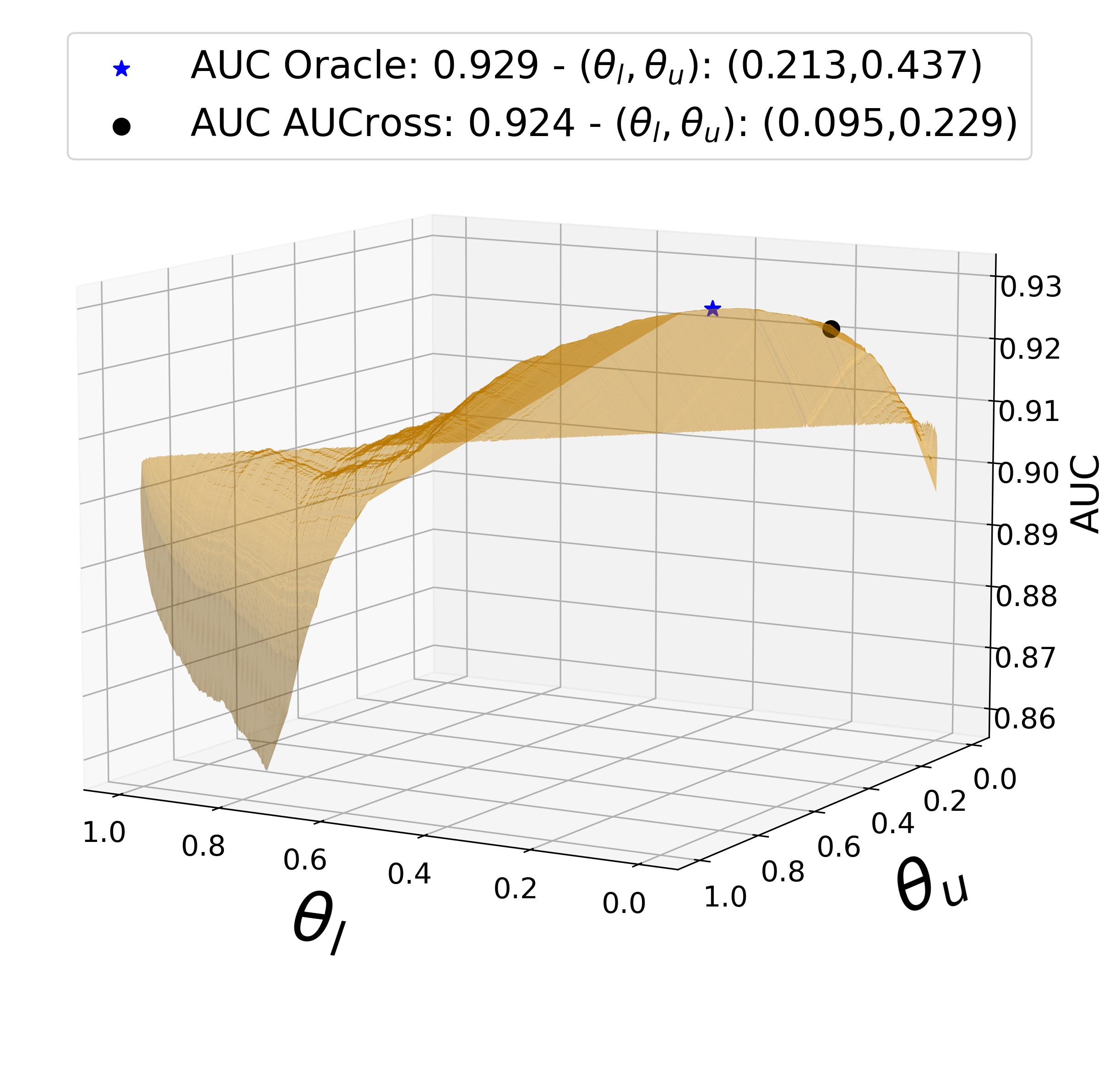
The first experiment evaluates how well the AUCross algorithm approximates the optimal solution to the problem of maximizing s.t. over the test set , considering the family of score-bounded selection functions. For tabular data, is fixed to a LightGBM classifier (Ke et al., 2017) with default hyperparameters. For image data, we used a VGG architecture as a base classifier (Simonyan and Zisserman, 2015), trained with cross-entropy loss. We enumerate all the score-bounded selection functions iff by varying the bounds such that . The Oracle approach chooses the function which maximizes . It requires knowing the true class of instances in ; hence it is not feasible in practice. Table 2 shows the difference between the empirical AUC () achieved by the Oracle and the one of AUCross on the test sets of the experimental datasets (the value of the empirical AUC for AUCross is reported in Table 3 and discussed later on). We notice that AUCross reaches the Oracle performance for the LendingClub and CatsVsDogs datasets. For the datasets Adult, CSDS1, CSDS3 and CIFAR-10-cat, there are larger violations for smaller ’s, while we do not see such a trend for GiveMe, UCICredit and CSDS2. This suggests that the strategy of centring the rejection area at a midpoint (line 15 of Alg. 2) might be sub-optimal. Figure 4 shows the performance over the space of bounds in a specific case, highlighting the bounds of Oracle and AUCross.
AUCross vs baselines
We compare the performance of AUCross to a few baselines. The first one is a bounded-improvement version of the plug-in rule (Herbei and Wegkamp, 2006) (PlugIn). PlugIn uses softmax as confidence function, i.e., in the binary case, , and it estimates the parameter as the quantile on a validation set. Such an approach requires splitting the training set into a dataset for building the classifier and a validation set for estimating (10% of the original dataset in our experiments). In contrast, AUCross allows for building the classifier using the whole training set. Second, we consider two hybrid versions of AUCross and PlugIn: (1) a plug-in rule specialized for AUC (PlugInAUC), i.e., that uses a score-bounded selection function by estimating bounds as in Alg. 1 on a validation set; (2) a cross-fitting version of PlugIn (called SCross by Pugnana and Ruggieri, 2023), where the selection function is softmax and the estimation of the bounds exploits the second-order improvement of of Thm. 4.
| Empirical Coverage | Selective AUC | ||||||||||||
| AUCross | PlugIn | PlugInAUC | SCross | SelNet | SAT | AUCross | PlugIn | PlugInAUC | SCross | SelNet | SAT | ||
| Adult | .99 | .989 .001 | .992 .001 | .991 .001 | .993 .001 | .985 .001 | .998 .001 | .929 .003 | .928 .003 | .928 .003 | .928 .003 | .901 .003 | .902 .003 |
| .95 | .950 .002 | .947 .002 | .950 .002 | .950 .002 | .954 .002 | .984 .002 | .935 .003 | .935 .003 | .934 .003 | .935 .003 | .907 .003 | .903 .003 | |
| .90 | .896 .003 | .900 .003 | .898 .003 | .904 .003 | .897 .003 | .966 .002 | .943 .002 | .941 .003 | .942 .003 | .941 .003 | .917 .003 | .904 .003 | |
| .85 | .849 .003 | .846 .003 | .850 .003 | .850 .003 | .772 .004 | .952 .002 | .950 .002 | .947 .003 | .949 .002 | .948 .003 | .848 .005 | .904 .003 | |
| .80 | .797 .004 | .794 .004 | .793 .004 | .802 .004 | .793 .004 | .934 .003 | .958 .002 | .952 .003 | .957 .002 | .953 .003 | .924 .004 | .904 .003 | |
| .75 | .750 .004 | .743 .004 | .744 .004 | .746 .004 | .736 .004 | .919 .003 | .963 .002 | .958 .003 | .962 .002 | .958 .003 | .917 .004 | .904 .003 | |
| Lending | .99 | .996 .001 | .995 .001 | .997 .001 | .994 .001 | .997 .001 | .073 .001 | .983 .001 | .984 .001 | .984 .001 | .983 .001 | .973 .001 | .664 .004 |
| .95 | .980 .001 | .970 .001 | .980 .001 | .969 .001 | .985 .001 | .073 .001 | .985 .001 | .985 .001 | .985 .001 | .984 .001 | .973 .001 | .664 .004 | |
| .90 | .959 .001 | .939 .001 | .958 .001 | .938 .001 | .928 .001 | .073 .001 | .987 .001 | .986 .001 | .987 .001 | .986 .001 | .981 .001 | .664 .004 | |
| .85 | .936 .001 | .909 .001 | .935 .001 | .908 .001 | .866 .001 | .073 .001 | .989 .001 | .988 .001 | .989 .001 | .987 .001 | .977 .001 | .664 .004 | |
| .80 | .912 .001 | .880 .001 | .911 .001 | .879 .001 | .850 .001 | .073 .001 | .990 .001 | .989 .001 | .991 .001 | .989 .001 | .991 .001 | .664 .004 | |
| .75 | .886 .001 | .850 .001 | .884 .001 | .849 .001 | .880 .001 | .073 .001 | .992 .001 | .990 .001 | .992 .001 | .990 .001 | .976 .001 | .664 .004 | |
| GiveMe | .99 | .990 .001 | .990 .001 | .990 .001 | .990 .001 | .944 .002 | .746 .003 | .868 .004 | .861 .004 | .869 .004 | .859 .004 | .747 .007 | .730 .006 |
| .95 | .950 .002 | .949 .002 | .947 .002 | .950 .002 | .944 .002 | .727 .003 | .874 .004 | .824 .006 | .875 .004 | .826 .006 | .748 .007 | .729 .006 | |
| .90 | .898 .002 | .903 .002 | .897 .002 | .902 .002 | .900 .002 | .705 .003 | .883 .004 | .784 .007 | .883 .004 | .784 .007 | .708 .008 | .728 .007 | |
| .85 | .848 .002 | .856 .002 | .849 .002 | .852 .002 | .848 .002 | .699 .003 | .890 .004 | .759 .008 | .890 .004 | .757 .008 | .658 .009 | .728 .007 | |
| .80 | .795 .003 | .807 .003 | .801 .003 | .800 .003 | .802 .003 | .694 .003 | .898 .004 | .744 .009 | .897 .004 | .743 .009 | .677 .009 | .727 .007 | |
| .75 | .748 .003 | .756 .003 | .750 .003 | .748 .003 | .754 .003 | .689 .003 | .904 .004 | .738 .010 | .904 .004 | .734 .010 | .676 .010 | .727 .007 | |
| UCICredit | .99 | .988 .002 | .993 .002 | .993 .001 | .993 .001 | .989 .002 | 1.000 .000 | .772 .008 | .772 .007 | .774 .007 | .770 .008 | .765 .007 | .768 .007 |
| .95 | .944 .003 | .948 .003 | .946 .003 | .951 .003 | .909 .004 | 1.000 .000 | .778 .008 | .769 .008 | .780 .007 | .765 .008 | .718 .009 | .768 .007 | |
| .90 | .896 .004 | .897 .004 | .900 .004 | .906 .004 | .904 .004 | .994 .001 | .785 .008 | .758 .008 | .787 .008 | .754 .009 | .707 .009 | .769 .007 | |
| .85 | .840 .005 | .851 .005 | .846 .005 | .848 .005 | .855 .005 | .994 .001 | .792 .008 | .746 .009 | .795 .008 | .734 .009 | .668 .009 | .769 .007 | |
| .80 | .789 .005 | .803 .005 | .797 .005 | .797 .005 | .810 .005 | .994 .001 | .800 .008 | .722 .010 | .802 .008 | .710 .010 | .644 .010 | .769 .007 | |
| .75 | .737 .006 | .751 .006 | .739 .006 | .750 .005 | .759 .005 | .994 .001 | .809 .008 | .695 .011 | .810 .008 | .679 .011 | .620 .011 | .769 .007 | |
| CSDS1 | .99 | .990 .001 | .980 .001 | .991 .001 | .980 .001 | .985 .001 | .984 .001 | .686 .003 | .675 .003 | .686 .003 | .675 .003 | .671 .003 | .669 .003 |
| .95 | .950 .001 | .918 .001 | .949 .001 | .917 .001 | .924 .001 | .937 .001 | .689 .003 | .654 .004 | .689 .003 | .655 .004 | .652 .004 | .654 .004 | |
| .90 | .898 .002 | .853 .002 | .898 .002 | .849 .002 | .863 .002 | .861 .002 | .693 .003 | .640 .004 | .694 .003 | .641 .004 | .638 .004 | .635 .004 | |
| .85 | .849 .002 | .792 .002 | .845 .002 | .790 .002 | .800 .002 | .803 .002 | .697 .003 | .631 .004 | .698 .003 | .631 .004 | .630 .004 | .625 .004 | |
| .80 | .799 .002 | .737 .002 | .795 .002 | .736 .002 | .740 .002 | .739 .002 | .702 .004 | .624 .004 | .703 .003 | .620 .004 | .618 .004 | .616 .004 | |
| .75 | .748 .002 | .681 .002 | .747 .002 | .682 .002 | .686 .002 | .687 .002 | .706 .004 | .613 .005 | .707 .004 | .616 .005 | .609 .005 | .608 .005 | |
| CSDS2 | .99 | .990 .001 | .984 .002 | .991 .001 | .983 .002 | .980 .002 | 1.000 .000 | .616 .020 | .585 .020 | .587 .020 | .616 .020 | .607 .020 | .623 .019 |
| .95 | .952 .002 | .927 .003 | .954 .002 | .916 .003 | .894 .003 | 1.000 .000 | .619 .020 | .572 .021 | .589 .020 | .581 .022 | .587 .022 | .623 .019 | |
| .90 | .904 .003 | .851 .004 | .907 .003 | .834 .004 | .805 .004 | .880 .003 | .620 .020 | .566 .023 | .590 .021 | .570 .023 | .560 .024 | .588 .022 | |
| .85 | .860 .004 | .773 .004 | .861 .004 | .761 .004 | .712 .005 | .817 .004 | .631 .021 | .552 .024 | .590 .021 | .572 .025 | .562 .026 | .589 .023 | |
| .80 | .811 .004 | .715 .005 | .818 .004 | .687 .005 | .663 .005 | .756 .004 | .631 .021 | .532 .025 | .592 .021 | .555 .026 | .547 .027 | .582 .024 | |
| .75 | .760 .004 | .651 .005 | .776 .004 | .620 .005 | .564 .005 | .697 .005 | .635 .021 | .536 .027 | .592 .021 | .541 .028 | .579 .029 | .575 .026 | |
| CSDS3 | .99 | .991 .001 | .992 .001 | .992 .001 | .991 .001 | .988 .001 | .992 .001 | .851 .003 | .850 .003 | .850 .003 | .850 .003 | .844 .003 | .844 .003 |
| .95 | .948 .002 | .957 .002 | .960 .002 | .955 .002 | .942 .002 | .951 .002 | .858 .003 | .852 .003 | .855 .003 | .853 .003 | .851 .003 | .849 .003 | |
| .90 | .901 .002 | .909 .002 | .909 .002 | .911 .002 | .913 .002 | .902 .002 | .865 .003 | .855 .003 | .863 .003 | .856 .004 | .850 .004 | .855 .004 | |
| .85 | .849 .003 | .859 .003 | .856 .003 | .865 .003 | .867 .003 | .856 .003 | .873 .003 | .857 .004 | .871 .003 | .858 .004 | .851 .004 | .858 .004 | |
| .80 | .805 .003 | .808 .003 | .811 .003 | .818 .003 | .796 .003 | .819 .003 | .880 .003 | .859 .004 | .878 .003 | .859 .004 | .859 .004 | .858 .004 | |
| .75 | .759 .003 | .758 .003 | .765 .003 | .769 .003 | .765 .003 | .776 .003 | .887 .003 | .858 .004 | .884 .003 | .859 .004 | .843 .004 | .853 .004 | |
| CatsVsDogs | .99 | .992 .002 | .990 .002 | .991 .002 | .992 .002 | .991 .002 | .993 .002 | .984 .003 | .985 .002 | .985 .002 | .985 .002 | .979 .003 | .985 .002 |
| .95 | .962 .003 | .965 .003 | .954 .004 | .959 .003 | .954 .003 | .959 .003 | .986 .003 | .985 .002 | .987 .002 | .987 .003 | .987 .002 | .987 .002 | |
| .90 | .920 .004 | .910 .004 | .907 .005 | .917 .004 | .891 .005 | .910 .005 | .987 .003 | .984 .002 | .988 .002 | .988 .003 | .990 .002 | .989 .002 | |
| .85 | .883 .005 | .854 .005 | .858 .005 | .871 .005 | .852 .006 | .862 .005 | .987 .003 | .984 .002 | .989 .002 | .988 .003 | .990 .002 | .990 .002 | |
| .80 | .841 .006 | .797 .006 | .805 .006 | .807 .006 | .809 .006 | .818 .006 | .987 .003 | .985 .002 | .990 .002 | .989 .003 | .991 .002 | .990 .002 | |
| .75 | .781 .006 | .740 .007 | .749 .007 | .744 .007 | .765 .007 | .768 .007 | .987 .003 | .983 .002 | .990 .002 | .988 .003 | .992 .002 | .990 .002 | |
| CIFAR10-CAT | .99 | 1.000 .001 | .991 .001 | .989 .002 | .992 .001 | .992 .001 | .990 .002 | .890 .009 | .915 .007 | .909 .008 | .922 .007 | .896 .008 | .893 .008 |
| .95 | .998 .001 | .950 .003 | .948 .003 | .953 .003 | .956 .003 | .952 .003 | .889 .009 | .895 .009 | .911 .007 | .906 .009 | .902 .008 | .863 .011 | |
| .90 | .994 .001 | .899 .004 | .898 .003 | .903 .003 | .904 .003 | .913 .003 | .889 .009 | .896 .009 | .913 .007 | .851 .013 | .899 .010 | .760 .017 | |
| .85 | .987 .002 | .849 .004 | .851 .004 | .886 .004 | .863 .004 | .854 .004 | .888 .009 | .898 .009 | .916 .007 | .815 .016 | .676 .022 | .574 .024 | |
| .80 | .969 .002 | .796 .005 | .799 .004 | .882 .004 | .806 .005 | .803 .005 | .885 .009 | .906 .008 | .919 .007 | .804 .017 | .359 .026 | .572 .024 | |
| .75 | .945 .003 | .749 .005 | .749 .005 | .879 .004 | .763 .005 | .759 .005 | .870 .011 | .905 .008 | .921 .007 | .797 .018 | .408 .028 | .575 .025 | |
| # | 21/54 | 12/54 | 8/54 | 15/54 | 8/54 | 1/54 | 28/54 | 4/54 | 29/54 | 6/54 | 5/54 | 2/54 | |
| .026 .046 | .021 .029 | .013 .026 | .028 .036 | .029 .041 | .171 .251 | ||||||||
These two variants allow us to evaluate the relative contributions of the two key elements of our approach: the estimation of AUC-specific bounds (Prop. 3), and the cross fitting approach paired with the second-order quantile estimation strategy (Thm. 4). We also consider two state-of-the-art methods for selective classification, namely the SelectiveNet (Geifman and El-Yaniv, 2019) (SelNet), and the Self Adaptive Training (Huang et al., 2020) (SAT) methods. The approach from Shen et al., 2020 is not included in the baselines since it rejects the comparison of pairs of instances, while we focus on the rejection of predictions on instances in isolation.
For tabular data, SelNet and SAT are built using a ResNet structure (Gorishniy et al., 2021), while AUCross, PlugIn, PlugInAUC and SCross are based on a LightGBM classifier. We report in the Appendix results for other base classifiers. For CatsVsDogs, a VGG architecture (Simonyan and Zisserman, 2015) is used for all the methods. For all the DNN approaches, we set 300 epochs in training, Stochastic Gradient Descent as an optimizer, a learning rate of decreased by a factor every epochs, as in the original papers. All the parameters of base classifiers are left as the default ones. See the Appendix for details.
Table 3 shows performance metrics (mean stdev) evaluated on 1,000 bootstrap runs of the test set: the empirical coverage and the empirical AUC . Resorting to bootstrap allows for calculating standard errors of the metrics22 2 Other approaches include confidence intervals for AUC (DeLong et al., 1988; Cortes and Mohri, 2004; Goncalves et al., 2014) or direct estimation of its variance (Cleves, 2002). (Rajkomar et al., 2018). Moreover, it allows for quantifying the generalizability of the methods to perturbations of the test set. Additional results on the selective accuracy and the positive rate33 3 Positive rate in the accepted region, compared to the positive rate in the overall test set, measures fairness of the selection function w.r.t. the class labels. metrics are reported in the Appendix. Results in Table 3 show that AUCross achieves an empirical coverage close to the target in most of the cases for tabular data. The most significant violation occurs for LendingClub, where also all the other methods fail to reach the target coverage. In particular, SAT performs poorly on such a dataset. The other largest violation occurs for CIFAR-10-cat. Here, also the other cross-fitting-based algorithm (SCross) fails to reach the target one. Interestingly, the runner-up method w.r.t. coverage is PlugInAUC, which has the smallest average violation. A striking case is the CSDS2 dataset, which is the most imbalanced one with a positive rate of 1.8%. Here, both AUCross and PlugInAUC have small violations, while all other approaches have larger ones. We argue that this is due to the bounds determined by Prop. 1 and Prop. 2, which are specific for positives and negatives, respectively, while the other methods calibrate the selection function independently of the class labels. Regarding the empirical AUC, AUCross and PlugInAUC outperform the other methods in most cases. For unbalanced datasets such as for GiveMe, CSDS1 and CSDS2, the empirical AUC drops for smaller coverages, contrarily to what is expected. Such behaviour does not occur for those methods that estimate bounds specifically for the AUC, i.e. AUCross and PlugInAUC. We show in the Appendix that a trade-off exists in terms of selective accuracy, as both AUCross and PlugInAUC are outperformed concerning the accuracy over the accepted region. This is not surprising since they are optimizing the AUC metric, and it is well-known that accuracy and AUC cannot be jointly optimized (Cortes and Mohri, 2003). The results in the Appendix also show that optimizing accuracy compromises the positive rate, while our approach is fairer in this sense.
Finally, consider the running time performances (see the Appendix for details). AUCross and SCross require executions of the base classifier (loop at lines 3-6 of Alg. 2), while all other baselines train a single (selective) classifier. On tabular data, using efficient base classifiers results in a reasonably low total running time. Those two strategies are instead computationally expensive for image data, where DNN base classifiers are adopted. However, we observe that PlugInAUC exhibits performances comparable to SelNet and SAT for CatsVsDogs, and it outperforms them in the case of CIFAR-10-cat. In summary, we recommend using AUCross for tabular datasets and PlugInAUC for image datasets.
7 CONCLUSIONS
Selective classification can help prevent poor or even harmful decisions by abstaining from making an output, possibly demanding the decision to a human. We have extended the selective classification framework to a widely used classifier evaluation metric, the Area Under the ROC Curve. Through an analytic characterization, we devised methods for computing an estimator of the best score-bounded selection function. These methods are effective and outperform existing approaches designed for optimizing accuracy.
Limitations that require future work include the following. First, the approach should be extended to multi-class classification, for which the notion of AUC has been considered, e.g., the Volume Under the Surface (Ferri et al., 2003), the average of pairwise binary AUCs (the M metric) (Hand and Till, 2001), or the AUC- (Kleiman and Page, 2019). Second, since selective classification might amplify unfair decisions (Jones et al., 2021), we intend to study how to account for fairness metrics in the context of AUC-based selective classification. Third, as suggested by our experimental results, we could better determine the bounds for a target coverage , reconsidering the choice of centring the rejection area in the midpoint of the bounds of Prop. 3. As shown in Table 2, this is especially relevant for large ’s. Lastly, AUC-based selective classification can be extended to the metric of weighted AUC (Fawcett, 2006b; Keilwagen et al., 2014), where instances are weighted by importance.
Reproducibility
Data and source code can be downloaded from https://github.com/andrepugni/AUCbasedSelectiveClassification.
Acknowledgements
Work supported by the XAI project, funded by the European Union’s Horizon 2020 Excellent Science European Research Council (ERC) programme under g.a. No. 834756. Views and opinions expressed are however those of the authors only and do not necessarily reflect those of the EU. Neither the EU nor the granting authority can be held responsible for them.
References
- Barddal et al., (2020) Barddal, J. P., Loezer, L., Enembreck, F., and Lanzuolo, R. (2020). Lessons learned from data stream classification applied to credit scoring. Expert Syst. Appl., 162:113899.
- Chernozhukov et al., (2018) Chernozhukov, V., Chetverikov, D., Demirer, M., Duflo, E., Hansen, C., Newey, W., and Robins, J. (2018). Double/debiased machine learning for treatment and structural parameters. The Econometrics Journal, 21(1):C1–C68.
- Chow, (1970) Chow, C. K. (1970). On optimum recognition error and reject tradeoff. IEEE Trans. Inf. Theory, 16(1):41–46.
- Cleves, (2002) Cleves, M. A. (2002). Comparative assessment of three common algorithms for estimating the variance of the area under the nonparametric receiver operating characteristic curve. The Stata Journal, 2:280–289.
- Cortes et al., (2016) Cortes, C., DeSalvo, G., and Mohri, M. (2016). Boosting with abstention. In NIPS, pages 1660–1668.
- Cortes and Mohri, (2003) Cortes, C. and Mohri, M. (2003). AUC optimization vs. error rate minimization. In NIPS, pages 313–320. MIT Press.
- Cortes and Mohri, (2004) Cortes, C. and Mohri, M. (2004). Confidence intervals for the area under the ROC curve. In NIPS, pages 305–312.
- DeLong et al., (1988) DeLong, E. R., DeLong, D. M., and Clarke-Pearson, D. L. (1988). Comparing the areas under two or more correlated receiver operating characteristic curves: A nonparametric approach. Biometrics, 44(3):837–845.
- Dua and Graff, (2017) Dua, D. and Graff, C. (2017). UCI machine learning repository.
- El-Yaniv and Wiener, (2010) El-Yaniv, R. and Wiener, Y. (2010). On the foundations of noise-free selective classification. J. Mach. Learn. Res., 11:1605–1641.
- Engelmann, (2011) Engelmann, B. (2011). Measures of a rating’s discriminative power: Applications and limitations. In Engelmann, B. and Rauhmeier, R., editors, The Basel II Risk Parameters, pages 269–291. Springer, 2 edition.
- (12) Fawcett, T. (2006a). An introduction to ROC analysis. Pattern Recognit. Lett., 27(8):861–874.
- (13) Fawcett, T. (2006b). ROC graphs with instance-varying costs. Pattern Recognit. Lett., 27(8):882–891.
- Ferri et al., (2003) Ferri, C., Hernández-Orallo, J., and Salido, M. A. (2003). Volume under the ROC surface for multi-class problems. In ECML, volume 2837 of Lecture Notes in Computer Science, pages 108–120. Springer.
- Franc and Průša, (2019) Franc, V. and Průša, D. (2019). On discriminative learning of prediction uncertainty. In ICML, volume 97 of Proceedings of Machine Learning Research, pages 1963–1971. PMLR.
- Fumera and Roli, (2002) Fumera, G. and Roli, F. (2002). Support vector machines with embedded reject option. In SVM, volume 2388 of Lecture Notes in Computer Science, pages 68–82. Springer.
- Geifman and El-Yaniv, (2017) Geifman, Y. and El-Yaniv, R. (2017). Selective classification for deep neural networks. In NIPS, pages 4878–4887.
- Geifman and El-Yaniv, (2019) Geifman, Y. and El-Yaniv, R. (2019). Selectivenet: A deep neural network with an integrated reject option. In ICML, volume 97 of Proceedings of Machine Learning Research, pages 2151–2159. PMLR.
- Goncalves et al., (2014) Goncalves, L., Subtil, A., Oliveira, M. R., and de Zea Bermudez, P. (2014). ROC curve estimation: An overview. Revstat - Statistical Journal, 12:1–20.
- Gorishniy et al., (2021) Gorishniy, Y., Rubachev, I., Khrulkov, V., and Babenko, A. (2021). Revisiting deep learning models for tabular data. In NeurIPS, pages 18932–18943.
- Hand and Till, (2001) Hand, D. J. and Till, R. J. (2001). A simple generalisation of the area under the ROC curve for multiple class classification problems. Mach. Learn., 45(2):171–186.
- Hendrickx et al., (2021) Hendrickx, K., Perini, L., der Plas, D. V., Meert, W., and Davis, J. (2021). Machine learning with a reject option: A survey. CoRR, abs/2107.11277.
- Herbei and Wegkamp, (2006) Herbei, R. and Wegkamp, M. H. (2006). Classification with reject option. Can. J. Stat., 34(4):709–721.
- Huang and Ling, (2005) Huang, J. and Ling, C. X. (2005). Using AUC and accuracy in evaluating learning algorithms. IEEE Trans. Knowl. Data Eng., 17(3):299–310.
- Huang et al., (2020) Huang, L., Zhang, C., and Zhang, H. (2020). Self-adaptive training: beyond empirical risk minimization. In NeurIPS.
- Jones et al., (2021) Jones, E., Sagawa, S., Koh, P. W., Kumar, A., and Liang, P. (2021). Selective classification can magnify disparities across groups. In ICLR. OpenReview.net.
- Ke et al., (2017) Ke, G., Meng, Q., Finley, T., Wang, T., Chen, W., Ma, W., Ye, Q., and Liu, T. (2017). LightGBM: A highly efficient gradient boosting decision tree. In NIPS, pages 3146–3154.
- Keilwagen et al., (2014) Keilwagen, J., Grosse, I., and Grau, J. (2014). Area under precision-recall curves for weighted and unweighted data. PLoS ONE, 9(3):e92209.
- Kleiman and Page, (2019) Kleiman, R. and Page, D. (2019). AUC: A performance metric for multi-class machine learning models. In ICML, volume 97 of Proceedings of Machine Learning Research, pages 3439–3447. PMLR.
- Knight and Bassett, (2003) Knight, K. and Bassett, G. W. (2003). Second order improvements of sample quantiles using subsamples. Unpublished manuscript, http://www.utstat.toronto.edu/keith/papers/subsample.pdf.
- Krizhevsky, (2009) Krizhevsky, A. (2009). Learning multiple layers of features from tiny images. Technical report, University of Toronto.
- Liu et al., (2019) Liu, Z., Wang, Z., Liang, P. P., Salakhutdinov, R., Morency, L., and Ueda, M. (2019). Deep gamblers: Learning to abstain with portfolio theory. In NeurIPS, pages 10622–10632.
- Pietraszek, (2005) Pietraszek, T. (2005). Optimizing abstaining classifiers using ROC analysis. In ICML, volume 119 of ACM International Conference Proceeding Series, pages 665–672. ACM.
- Pugnana and Ruggieri, (2023) Pugnana, A. and Ruggieri, S. (2023). A model-agnostic heuristics for selective classification. In AAAI. AAAI Press.
- Rajkomar et al., (2018) Rajkomar, A., Oren, E., Chen, K., Dai, A. M., Hajaj, N., Hardt, M., Liu, P. J., Liu, X., Marcus, J., Sun, M., et al. (2018). Scalable and accurate deep learning with electronic health records. NPJ Digital Medicine, 1(1):1–10.
- Shen et al., (2020) Shen, S., Yang, B., and Gao, W. (2020). AUC optimization with a reject option. In AAAI, pages 5684–5691. AAAI Press.
- Simonyan and Zisserman, (2015) Simonyan, K. and Zisserman, A. (2015). Very deep convolutional networks for large-scale image recognition. In ICLR.
- Tortorella, (2005) Tortorella, F. (2005). A ROC-based reject rule for dichotomizers. Pattern Recognit. Lett., 26(2):167–180.
- Vovk, (2013) Vovk, V. (2013). Conditional validity of inductive conformal predictors. Mach. Learn., 92(2-3):349–376.
- Wu and Lee, (2014) Wu, Y.-C. and Lee, W.-C. (2014). Alternative performance measures for prediction models. PLoS ONE, 9(3):e91249.
- Yang and Ying, (2023) Yang, T. and Ying, Y. (2023). AUC maximization in the era of big data and AI: A survey. ACM Comput. Surv., 55(8):172:1–172:37.
- Yeh and Lien, (2009) Yeh, I. and Lien, C. (2009). The comparisons of data mining techniques for the predictive accuracy of probability of default of credit card clients. Expert Syst. Appl., 36(2):2473–2480.
Supplementary Materials for AUC-based selective classification
Appendix A APPENDIX
A.1 Proofs
Proposition 1.
Proof.
The missing part of the proof consists of the following equivalence:
| iff | ||||
| iff | ||||
| iff | ||||
| iff | ||||
| iff | ||||
| iff | ||||
| iff | ||||
| iff | ||||
| iff | ||||
| iff | ||||
| iff | ||||
| iff |
∎
Proposition 2.
Proof.
We can equivalently show the result for the Gini coefficient. Let , and let be the Gini coefficient after removing (a.k.a., abstaining on) one negative instance . We have . Then iff
| (11) |
As in Proposition 1, we can link the area after the removal of the negative instance to the original area as follows:
As for the positive case, this can be intuitively understood by looking at Figure 5, where the grey area highlights the loss from the original CAP plot after we remove the negative instance. Then we rescale to account for the new number of instances, as in Figure 6. Then:
| iff | ||||
| iff | ||||
| iff | ||||
| iff | ||||
| iff | ||||
| iff |
Since , and
| (12) |
is assumed to hold, we have the (a.k.a., the conclusion of Proposition 2) after removing one negative instance. Moreover, if (12) holds for a second negative instance , then:
where abstains on the first negative instance. In fact, implies that . Therefore, we can iterate the conclusion that the Gini coefficient (or, equivalently, empirical AUC) increases by abstaining on any number of negative instances that satisfy the assumption of Proposition 2. ∎


A.2 Datasets description
Adult is an extract from the 1994 US Census, with class the binarization of income into and . The final training set contains 30,162 instances and 55 features after one-hot encoding. The test set size is 15,060.
LendingClub regards repaying a loan obtained by an online platform. We used a temporal split to build the final training set (1,364,697 instances) and the test set (445,912 instances). The dataset has 65 features.
The GiveMe dataset aims at predicting the financial distress of a borrower within two years. The training and the test set were obtained by stratified random sampling, and they contain 12 features, and 112,500 and 37,500 instances respectively.
UCICredit regards credit card defaults in Taiwan. This dataset from Dua and Graff, 2017 concerns whether or not a credit card holder will default in the next six months (Yeh and Lien, 2009). Training and test sets were obtained by stratified random sampling. The training set includes 22,500 instances (7,500 for the test set) and 23 features.
CSDS1, CSDS2 and CSDS3 - from Barddal et al., 2020 - regard predicting defaults in repaying a loan: within six months for CSDS1 (data span over 15 months), within 2 months for CSDS2 (data span over 25 months), and within three months for CSDS3 (data span over 16 months). Training set and test set were divided through a timestamp variable. The training set of CSDS1 consists of 230,409 instances and 155 features (test set size is 76,939). For CSDS2, the training set contains 37,100 instances and 35 features (test set size is 12,533). For CSDS3, the training set contains 71,177 instances and 144 features (test set size 23,288).
The CatsVsDogs dataset is a collection of cats and dogs images. The task here is to distinguish between the two species. The training and test sets were obtained as described in Liu et al., 2019. The training set contains 20,000 images, each one of 64x64 pixels. The test set consists of 5,000 images.
Finally we considered the image dataset CIFAR-10-cat from Krizhevsky, 2009. For each of the 10 class labels, we have 5,000 32x32 images in the training set and 1,000 in the test set. We transformed it into a binary classification task by using the cat label as the positive class.
A.3 Models
AUCross and PlugInAUC.
In the main paper we used as base classifier a LightGBM classifier with default parameters. In Tables 6-9 we provide also results for a Logistic Regression and a Random Forest Classifier from sklearn package with default parameters, a ResNet implementation with default parameters from rtdl (Gorishniy et al., 2021) and a XGBoost from xgboost package with default parameters.
PlugIn and SCross.
As for AUCross, we considered a LightGBM classifier with default parameters.
SelNet.

Selective Net is a selective model that optimizes at the same time both and . Its schema is summarized in Figure 7. The architecture is based on four distinct parts: the main body, the predictive head, the selective head and the auxiliary head. The input is initially processed by the main body: it consists of deep layers that are shared by all the three heads. Any type of architecture can be used in this part (e.g., convolutional layers, linear layers, recurrent layers ecc.). The predictive head provides the final prediction ; the selective head outputs the selective function ; the auxiliary head is used to ensure that the main body part is exposed to all training instances, i.e., it is used to avoid that SelNet overfits on the accepted instances. We used pytorch to model SelNet. For tabular datasets, we built the main body part using ResNet with default parameters provided by rtdl (Gorishniy et al., 2021), as authors claim that ResNet is a valid baseline on tabular data. For images, we used as the main body the VGG16 architecture (Simonyan and Zisserman, 2015) as done in the original paper (Geifman and El-Yaniv, 2019). We then added the classification head, the selection head and the auxiliary head following SelNet paper. For CSDS1, Lending and GiveMe the prediction head and the auxiliary head were made by a first linear layer with 512 nodes followed by a batch normalization layer and ReLu activation; a second layer with 256 nodes, batch normalization and ReLu activation; a final dense layer with 128 nodes ending with two nodes and softmax activation. For the other datasets the classification and auxiliary heads were made by a single linear layer with 128 nodes and a final softmax activation. We built selective heads using a linear layer with 128 nodes, batch normalization, relu activation and another 64-node linear layer ending with a single node and Sigmoid activation. All the models are available in the code here. We point out that the lack of a clear design methodology of the SelectiveNet structure for a given dataset is a major drawback of SelNet compared to the flexibility our model-agnostic method. Models were trained, for an expected coverage , using the same loss function as in Geifman and El-Yaniv, 2019:
| (13) |
where is the classification head prediction, is the cross entropy loss, is the selection head output over instance , is the auxiliary head prediction and is the empirical coverage. Both parameters and are set as in Geifman and El-Yaniv, 2019 to and . The batch size was for Lending; for GiveMe, CSDS1, CSDS2, CSDS3 and image data; for Adult and UCICredit. The learning procedure was run for 300 epochs with 13 as loss and it used as an optimizer Stochastic Gradient Descent setting learning-rate=.1, momentum=.9,Nesterov=True and a decay of every 25 epochs as in the original paper. The training was performed over 90% of training set instances while we used the remaining 10% to calibrate the selective head.
SAT.
Let us consider the standard binary classification problem where the classifier can produce a score for instance belonging to class or 44 4 The problem is symmetrical in the binary setting., i.e. in our main paper . SAT Huang et al., 2020 introduces an extra class (representing abstention) during training and replace the confidence function with the score for the additional class . This allows for training a selective classifier in an end-to-end fashion. Given a batch of data pairs of size , the model score for class , and its exponential moving average for each sample, we optimize the classifier by minimizing:
| (14) |
where denotes the score attributed by the classifier to the true class of instance . This loss is a composition of two terms: the first one measures the standard cross-entropy loss between prediction and original label ; the second term acts as the selection function and identifies uncertain samples in the dataset. The value trades-off these two terms: if is very small, the sample is treated as uncertain and the second term enforces the selective classifier to learn to abstain from this sample; if is close to 1, the loss recovers the standard cross entropy minimization and enforces the selective classifier to make perfect predictions. The code was based on the pytorch implementation available here. We employed the same batch sizes as for SelNet and we set up training details as in the original paper of SAT: we used the loss in 14 for 300 epochs and as an optimizer Stochastic Gradient Descent, setting learning-rate=.1, momentum=.9,Nesterov=True and a decay of every 25 epochs. The training was performed over 90% of training set instances while we used the remaining 10% to calibrate the selection function.
A.4 Other metrics considered
We report results for selective accuracy and positive rate in Table 4. As discussed in the main paper, AUCross and PlugInAUC do not guarantee improvements in terms of accuracy whenever the target coverage decreases. Interestingly, they are able to maintain the positive rate more stable than the compared approaches. Finally, we report training times for all the methods in Table 5. PlugInAUC and PlugIn are clear winners over tabular datases as they can exploit fast classifiers. Both AUCross and SCross pay a factor proportional to the number of folds used in the cross-fitting part of the algorithm. This extra cost can be potentially mitigated on tabular datasets by parallelizing the cross-fitting procedure. Finally, notice that SelNet is the only approach which require a separate run for each target coverage .
| Selective Accuracy | Positive Rate | ||||||||||||
| AUCross | PlugIn | PlugInAUC | SCross | SelNet | SAT | AUCross | PlugIn | PlugInAUC | SCross | SelNet | SAT | ||
| Adult | .99 | .870 .003 | .872 .003 | .870 .003 | .871 .003 | .848 .003 | .845 .003 | .246 .004 | .245 .004 | .246 .004 | .245 .004 | .242 .004 | .246 .004 |
| .95 | .875 .003 | .888 .003 | .874 .003 | .888 .003 | .858 .003 | .845 .003 | .246 .004 | .234 .004 | .247 .004 | .234 .004 | .235 .004 | .247 .004 | |
| .90 | .882 .003 | .903 .003 | .880 .003 | .902 .003 | .872 .003 | .845 .003 | .246 .004 | .221 .004 | .248 .004 | .220 .004 | .225 .004 | .249 .004 | |
| .85 | .888 .003 | .920 .003 | .887 .003 | .919 .003 | .886 .003 | .846 .003 | .247 .004 | .203 .004 | .249 .004 | .206 .004 | .115 .003 | .250 .004 | |
| .80 | .899 .003 | .936 .003 | .897 .003 | .934 .003 | .901 .003 | .846 .003 | .245 .004 | .185 .004 | .249 .004 | .190 .004 | .180 .004 | .251 .004 | |
| .75 | .907 .003 | .950 .003 | .905 .003 | .950 .003 | .908 .003 | .845 .004 | .245 .005 | .169 .004 | .250 .005 | .170 .004 | .149 .004 | .252 .004 | |
| Lending | .99 | .899 .001 | .899 .001 | .899 .001 | .899 .001 | .870 .001 | .754 .003 | .224 .001 | .222 .001 | .224 .001 | .222 .001 | .223 .001 | .249 .003 |
| .95 | .908 .001 | .909 .001 | .909 .001 | .910 .001 | .873 .001 | .754 .003 | .217 .001 | .206 .001 | .217 .001 | .205 .001 | .215 .001 | .249 .003 | |
| .90 | .921 .001 | .923 .001 | .921 .001 | .924 .001 | .912 .001 | .754 .003 | .207 .001 | .184 .001 | .207 .001 | .183 .001 | .191 .001 | .249 .003 | |
| .85 | .934 .001 | .937 .001 | .934 .001 | .938 .001 | .885 .001 | .754 .003 | .197 .001 | .162 .001 | .197 .001 | .161 .001 | .134 .001 | .249 .003 | |
| .80 | .948 .001 | .951 .001 | .949 .001 | .951 .001 | .926 .001 | .754 .003 | .186 .001 | .140 .001 | .186 .001 | .139 .001 | .157 .001 | .249 .003 | |
| .75 | .964 .001 | .963 .001 | .965 .001 | .963 .001 | .924 .001 | .754 .003 | .174 .001 | .118 .001 | .174 .001 | .116 .001 | .143 .001 | .249 .003 | |
| GiveMe | .99 | .938 .002 | .942 .002 | .938 .002 | .942 .002 | .954 .002 | .916 .002 | .068 .002 | .063 .002 | .067 .002 | .063 .002 | .047 .002 | .085 .002 |
| .95 | .937 .002 | .956 .002 | .937 .002 | .956 .002 | .954 .002 | .915 .002 | .068 .002 | .046 .002 | .068 .002 | .047 .002 | .047 .002 | .086 .002 | |
| .90 | .938 .002 | .967 .001 | .937 .002 | .967 .001 | .961 .001 | .913 .002 | .067 .002 | .034 .001 | .068 .002 | .034 .001 | .040 .001 | .088 .002 | |
| .85 | .939 .002 | .973 .001 | .938 .002 | .973 .001 | .967 .001 | .913 .002 | .067 .002 | .028 .001 | .068 .002 | .028 .001 | .034 .001 | .088 .002 | |
| .80 | .939 .002 | .977 .001 | .938 .002 | .978 .001 | .969 .001 | .912 .002 | .067 .002 | .024 .001 | .067 .002 | .023 .001 | .032 .001 | .089 .002 | |
| .75 | .939 .002 | .980 .001 | .939 .002 | .981 .001 | .971 .001 | .912 .002 | .067 .002 | .021 .001 | .068 .002 | .020 .001 | .030 .001 | .089 .002 | |
| UCICredit | .99 | .811 .005 | .814 .005 | .812 .005 | .814 .005 | .815 .005 | .812 .005 | .222 .005 | .220 .005 | .222 .005 | .220 .005 | .220 .005 | .222 .005 |
| .95 | .810 .005 | .826 .005 | .811 .005 | .827 .005 | .824 .005 | .812 .005 | .225 .006 | .210 .005 | .224 .005 | .209 .005 | .180 .005 | .222 .005 | |
| .90 | .809 .005 | .838 .005 | .811 .005 | .839 .005 | .830 .005 | .813 .005 | .228 .006 | .194 .005 | .226 .006 | .195 .005 | .176 .005 | .221 .005 | |
| .85 | .806 .005 | .849 .005 | .811 .005 | .855 .005 | .845 .005 | .813 .005 | .233 .006 | .179 .005 | .229 .006 | .176 .005 | .156 .005 | .221 .005 | |
| .80 | .806 .006 | .863 .005 | .810 .006 | .867 .005 | .858 .005 | .813 .005 | .236 .006 | .161 .005 | .232 .006 | .158 .005 | .143 .005 | .221 .005 | |
| .75 | .806 .006 | .872 .005 | .808 .006 | .875 .005 | .871 .005 | .813 .005 | .239 .006 | .143 .005 | .237 .006 | .141 .005 | .130 .005 | .221 .005 | |
| CSDS1 | .99 | .857 .002 | .863 .002 | .857 .002 | .863 .002 | .861 .002 | .862 .002 | .145 .002 | .139 .002 | .144 .002 | .138 .002 | .140 .002 | .139 .002 |
| .95 | .856 .002 | .875 .002 | .856 .002 | .875 .002 | .873 .002 | .871 .002 | .146 .002 | .126 .002 | .146 .002 | .126 .002 | .128 .002 | .130 .002 | |
| .90 | .854 .002 | .885 .002 | .855 .002 | .885 .002 | .882 .002 | .883 .002 | .147 .002 | .116 .002 | .147 .002 | .116 .002 | .119 .002 | .118 .002 | |
| .85 | .853 .002 | .892 .002 | .853 .002 | .892 .002 | .890 .002 | .890 .002 | .149 .002 | .109 .002 | .149 .002 | .109 .002 | .111 .002 | .111 .002 | |
| .80 | .852 .002 | .898 .002 | .852 .002 | .899 .002 | .897 .002 | .897 .002 | .150 .002 | .103 .002 | .150 .002 | .102 .002 | .104 .002 | .104 .002 | |
| .75 | .850 .002 | .904 .002 | .850 .002 | .904 .002 | .902 .002 | .902 .002 | .152 .002 | .097 .002 | .152 .002 | .097 .002 | .099 .002 | .099 .002 | |
| CSDS2 | .99 | .982 .002 | .982 .002 | .982 .002 | .982 .002 | .983 .002 | .982 .002 | .019 .002 | .019 .002 | .019 .002 | .019 .002 | .018 .002 | .019 .002 |
| .95 | .982 .002 | .983 .002 | .982 .002 | .985 .002 | .984 .002 | .982 .002 | .019 .002 | .018 .002 | .019 .002 | .016 .002 | .017 .002 | .019 .002 | |
| .90 | .982 .002 | .984 .002 | .982 .002 | .985 .002 | .986 .002 | .985 .002 | .019 .002 | .017 .002 | .019 .002 | .016 .002 | .015 .002 | .016 .002 | |
| .85 | .982 .002 | .985 .002 | .981 .002 | .986 .002 | .986 .002 | .985 .002 | .019 .002 | .016 .002 | .019 .002 | .015 .002 | .015 .002 | .016 .002 | |
| .80 | .982 .002 | .986 .002 | .981 .002 | .987 .002 | .987 .002 | .986 .002 | .019 .002 | .015 .002 | .019 .002 | .014 .002 | .014 .002 | .015 .002 | |
| .75 | .981 .002 | .986 .002 | .981 .002 | .987 .002 | .988 .002 | .987 .002 | .019 .002 | .015 .002 | .020 .002 | .014 .002 | .013 .002 | .014 .002 | |
| CSDS3 | .99 | .814 .003 | .816 .003 | .813 .003 | .816 .003 | .810 .003 | .809 .003 | .253 .003 | .252 .003 | .254 .003 | .251 .003 | .251 .003 | .252 .003 |
| .95 | .817 .003 | .826 .003 | .816 .003 | .827 .003 | .822 .003 | .820 .003 | .254 .003 | .242 .003 | .254 .003 | .242 .003 | .244 .003 | .243 .003 | |
| .90 | .820 .003 | .841 .003 | .819 .003 | .841 .003 | .830 .003 | .835 .003 | .254 .003 | .228 .003 | .255 .003 | .229 .003 | .233 .003 | .232 .003 | |
| .85 | .825 .003 | .856 .003 | .823 .003 | .855 .003 | .844 .003 | .850 .003 | .254 .003 | .214 .003 | .255 .003 | .215 .003 | .219 .003 | .219 .003 | |
| .80 | .829 .003 | .871 .003 | .826 .003 | .869 .003 | .860 .003 | .861 .003 | .254 .004 | .199 .003 | .256 .004 | .200 .003 | .206 .003 | .207 .003 | |
| .75 | .835 .003 | .884 .003 | .830 .003 | .883 .003 | .871 .003 | .872 .003 | .254 .004 | .182 .003 | .257 .004 | .185 .003 | .178 .003 | .188 .003 | |
| CatsVsDogs | .99 | .954 .004 | .950 .004 | .944 .004 | .956 .003 | .941 .004 | .950 .004 | .500 .008 | .505 .008 | .503 .008 | .500 .008 | .500 .008 | .500 .008 |
| .95 | .968 .003 | .949 .004 | .953 .004 | .969 .003 | .964 .003 | .964 .003 | .498 .008 | .514 .008 | .512 .008 | .495 .008 | .494 .008 | .497 .008 | |
| .90 | .977 .003 | .947 .004 | .971 .003 | .979 .003 | .978 .003 | .977 .003 | .494 .008 | .531 .008 | .518 .008 | .490 .008 | .482 .008 | .496 .008 | |
| .85 | .984 .002 | .944 .004 | .982 .003 | .985 .002 | .983 .002 | .984 .002 | .488 .008 | .546 .008 | .524 .008 | .488 .008 | .485 .008 | .494 .008 | |
| .80 | .987 .002 | .942 .004 | .986 .002 | .989 .002 | .990 .002 | .985 .002 | .473 .008 | .556 .008 | .528 .008 | .493 .008 | .476 .008 | .482 .008 | |
| .75 | .988 .002 | .938 .004 | .988 .002 | .990 .002 | .990 .002 | .987 .002 | .445 .008 | .561 .009 | .529 .009 | .500 .009 | .472 .008 | .464 .008 | |
| CIFAR10-CAT | .99 | .952 .003 | .952 .003 | .953 .003 | .956 .002 | .952 .003 | .958 .002 | .101 .004 | .092 .003 | .102 .004 | .097 .004 | .098 .004 | .096 .004 |
| .95 | .952 .003 | .952 .003 | .951 .003 | .969 .002 | .967 .002 | .969 .002 | .100 .004 | .072 .003 | .106 .004 | .078 .003 | .084 .003 | .075 .003 | |
| .90 | .953 .003 | .950 .003 | .950 .003 | .977 .002 | .977 .002 | .973 .002 | .100 .004 | .074 .003 | .111 .004 | .049 .003 | .064 .003 | .044 .003 | |
| .85 | .954 .003 | .947 .003 | .948 .003 | .979 .002 | .977 .002 | .976 .002 | .099 .004 | .077 .003 | .115 .004 | .040 .003 | .024 .002 | .025 .002 | |
| .80 | .959 .003 | .945 .003 | .946 .003 | .980 .002 | .984 .002 | .975 .002 | .095 .004 | .080 .004 | .122 .004 | .037 .003 | .017 .002 | .026 .002 | |
| .75 | .971 .002 | .942 .003 | .943 .003 | .980 .002 | .986 .002 | .975 .002 | .084 .003 | .084 .004 | .129 .004 | .036 .003 | .015 .002 | .026 .002 | |
| # | 4/54 | 21/54 | 2/54 | 29/54 | 12/54 | 3/54 | 39/54 | 4/54 | 20/54 | 5/54 | 1/54 | 14/54 | |
| Training Time (seconds) | |||||||
| AUCross | Plug-In | Plug-In-AUC | SCross | SelNet | SAT | ||
| Adult | .99 | 1.43 | 0.22 | 0.22 | 1.15 | 1787.93 | 2319.66 |
| .95 | 1.43 | 0.22 | 0.22 | 1.15 | 1779.74 | 2319.66 | |
| .90 | 1.43 | 0.22 | 0.22 | 1.15 | 1786.99 | 2319.66 | |
| .85 | 1.43 | 0.22 | 0.22 | 1.15 | 1781.64 | 2319.66 | |
| .80 | 1.43 | 0.22 | 0.22 | 1.15 | 1789.44 | 2319.66 | |
| .75 | 1.43 | 0.22 | 0.22 | 1.15 | 1788.53 | 2319.66 | |
| Lending | .99 | 13.16 | 2.55 | 2.55 | 12.10 | 9168.31 | 14182.26 |
| .95 | 13.16 | 2.55 | 2.55 | 12.10 | 9198.68 | 14182.26 | |
| .90 | 13.16 | 2.55 | 2.55 | 12.10 | 9187.33 | 14182.26 | |
| .85 | 13.16 | 2.55 | 2.55 | 12.10 | 9204.72 | 14182.26 | |
| .80 | 13.16 | 2.55 | 2.55 | 12.10 | 9165.67 | 14182.26 | |
| .75 | 13.16 | 2.55 | 2.55 | 12.10 | 9199.28 | 14182.26 | |
| GiveMe | .99 | 1.60 | 0.27 | 0.27 | 1.39 | 2341.00 | 3104.83 |
| .95 | 1.60 | 0.27 | 0.27 | 1.39 | 2323.07 | 3104.83 | |
| .90 | 1.60 | 0.27 | 0.27 | 1.39 | 2332.69 | 3104.83 | |
| .85 | 1.60 | 0.27 | 0.27 | 1.39 | 2332.97 | 3104.83 | |
| .80 | 1.60 | 0.27 | 0.27 | 1.39 | 2326.58 | 3104.83 | |
| .75 | 1.60 | 0.27 | 0.27 | 1.39 | 2333.06 | 3104.83 | |
| UCICredit | .99 | 1.26 | 0.20 | 0.20 | 1.11 | 1547.44 | 2070.54 |
| .95 | 1.26 | 0.20 | 0.20 | 1.11 | 1549.75 | 2070.54 | |
| .90 | 1.26 | 0.20 | 0.20 | 1.11 | 1527.84 | 2070.54 | |
| .85 | 1.26 | 0.20 | 0.20 | 1.11 | 1547.15 | 2070.54 | |
| .80 | 1.26 | 0.20 | 0.20 | 1.11 | 1548.82 | 2070.54 | |
| .75 | 1.26 | 0.20 | 0.20 | 1.11 | 1541.74 | 2070.54 | |
| CSDS1 | .99 | 5.60 | 1.02 | 1.02 | 5.31 | 4815.42 | 5524.00 |
| .95 | 5.60 | 1.02 | 1.02 | 5.31 | 4812.96 | 5524.00 | |
| .90 | 5.60 | 1.02 | 1.02 | 5.31 | 4813.66 | 5524.00 | |
| .85 | 5.60 | 1.02 | 1.02 | 5.31 | 4817.26 | 5524.00 | |
| .80 | 5.60 | 1.02 | 1.02 | 5.31 | 4818.25 | 5524.00 | |
| .75 | 5.60 | 1.02 | 1.02 | 5.31 | 4812.89 | 5524.00 | |
| CSDS2 | .99 | 1.23 | 0.21 | 0.21 | 1.41 | 609.99 | 357.92 |
| .95 | 1.23 | 0.21 | 0.21 | 1.41 | 609.32 | 357.92 | |
| .90 | 1.23 | 0.21 | 0.21 | 1.41 | 606.45 | 357.92 | |
| .85 | 1.23 | 0.21 | 0.21 | 1.41 | 606.47 | 357.92 | |
| .80 | 1.23 | 0.21 | 0.21 | 1.41 | 610.34 | 357.92 | |
| .75 | 1.23 | 0.21 | 0.21 | 1.41 | 605.20 | 357.92 | |
| CSDS3 | .99 | 5.07 | 0.80 | 0.80 | 4.60 | 1188.31 | 748.88 |
| .95 | 5.07 | 0.80 | 0.80 | 4.60 | 1193.35 | 748.88 | |
| .90 | 5.07 | 0.80 | 0.80 | 4.60 | 1192.50 | 748.88 | |
| .85 | 5.07 | 0.80 | 0.80 | 4.60 | 1190.79 | 748.88 | |
| .80 | 5.07 | 0.80 | 0.80 | 4.60 | 1191.03 | 748.88 | |
| .75 | 5.07 | 0.80 | 0.80 | 4.60 | 1191.56 | 748.88 | |
| CatsVsDogs | .99 | 14668.55 | 2624.68 | 2624.68 | 14475.64 | 2700.46 | 2735.28 |
| .95 | 14668.55 | 2624.68 | 2624.68 | 14475.64 | 2699.13 | 2735.28 | |
| .90 | 14668.55 | 2624.68 | 2624.68 | 14475.64 | 2733.35 | 2735.28 | |
| .85 | 14668.55 | 2624.68 | 2624.68 | 14475.64 | 2769.44 | 2735.28 | |
| .80 | 14668.55 | 2624.68 | 2624.68 | 14475.64 | 2766.80 | 2735.28 | |
| .75 | 14668.55 | 2624.68 | 2624.68 | 14475.64 | 2762.34 | 2735.28 | |
| CIFAR10-CAT | .99 | 17401.61 | 3026.98 | 3026.98 | 16924.30 | 3317.14 | 3239.50 |
| .95 | 17401.61 | 3026.98 | 3026.98 | 16924.30 | 3296.70 | 3239.50 | |
| .90 | 17401.61 | 3026.98 | 3026.98 | 16924.30 | 3337.28 | 3239.50 | |
| .85 | 17401.61 | 3026.98 | 3026.98 | 16924.30 | 3358.18 | 3239.50 | |
| .80 | 17401.61 | 3026.98 | 3026.98 | 16924.30 | 3262.57 | 3239.50 | |
| .75 | 17401.61 | 3026.98 | 3026.98 | 16924.30 | 3294.08 | 3239.50 | |
| # | 0/54 | 54/54 | 54/54 | 0/54 | 0/54 | 0/54 | |
A.5 Results for different classifiers
We report in Tables 6-9 the results for AUCross and PlugInAUC using different classifiers over tabular datasets. Regarding coverage, we see the harshest violations for both AUCross-RandForest and PlugInAUC-RandForest over CSDS2 and for AUCross-ResNet over GiveMe. Coverage violations occur also for Lending dataset, independently of the classifier. Regarding the AUC, both AUCross and PlugInAUC succeed in increasing it while target coverage drops, regardless of the considered base classifier. At the same time, we notice that for all the base classifiers lowering coverage does not guarantee selective accuracy to increase, highlighting once more the trade-off between these two metrics. Finally, we see similar results across all the classifiers for positive rate.
A.6 Results for different ’s
We report empirical coverage and selective AUC for different choices of the parameter in Table 10. The default value shows a slightly better trade-off between empirical coverage and selectice AUC.
| Empirical Coverage | |||||||||
| AUCross | PlugInAUC | ||||||||
| Logistic | RandForest | ResNet | XGBoost | Logistic | RandForest | ResNet | XGBoost | ||
| Adult | .99 | .991 (.001) | .988 (.001) | .994 (.001) | .990 (.001) | .988 (.001) | .989 (.001) | .988 (.001) | .992 (.001) |
| .95 | .950 (.002) | .945 (.002) | .961 (.002) | .951 (.002) | .947 (.002) | .949 (.002) | .946 (.002) | .951 (.002) | |
| .90 | .901 (.003) | .893 (.003) | .912 (.003) | .891 (.003) | .896 (.003) | .894 (.003) | .903 (.003) | .899 (.003) | |
| .85 | .850 (.003) | .853 (.003) | .840 (.004) | .846 (.003) | .848 (.003) | .836 (.004) | .849 (.003) | .850 (.003) | |
| .80 | .800 (.004) | .804 (.004) | .792 (.004) | .793 (.004) | .799 (.004) | .783 (.004) | .801 (.004) | .800 (.004) | |
| .75 | .747 (.004) | .752 (.004) | .735 (.004) | .744 (.004) | .744 (.004) | .743 (.004) | .749 (.004) | .748 (.004) | |
| Lending | .99 | .996 (.001) | .992 (.001) | .995 (.001) | .996 (.001) | .996 (.001) | .992 (.001) | .995 (.001) | .996 (.001) |
| .95 | .976 (.001) | .971 (.001) | .976 (.001) | .980 (.001) | .976 (.001) | .971 (.001) | .975 (.001) | .980 (.001) | |
| .90 | .951 (.001) | .945 (.001) | .951 (.001) | .958 (.001) | .951 (.001) | .945 (.001) | .949 (.001) | .958 (.001) | |
| .85 | .926 (.001) | .918 (.001) | .925 (.001) | .936 (.001) | .926 (.001) | .917 (.001) | .922 (.001) | .936 (.001) | |
| .80 | .900 (.001) | .890 (.001) | .898 (.001) | .912 (.001) | .899 (.001) | .884 (.001) | .894 (.001) | .912 (.001) | |
| .75 | .871 (.001) | .856 (.001) | .868 (.001) | .886 (.001) | .871 (.001) | .855 (.001) | .865 (.001) | .886 (.001) | |
| GiveMe | .99 | .990 (.001) | .942 (.002) | .944 (.002) | .990 (.001) | .991 (.001) | .944 (.002) | .977 (.001) | .991 (.001) |
| .95 | .953 (.002) | .942 (.002) | .755 (.003) | .951 (.002) | .950 (.002) | .944 (.002) | .930 (.002) | .948 (.002) | |
| .90 | .904 (.002) | .858 (.002) | .640 (.003) | .898 (.002) | .898 (.002) | .863 (.002) | .884 (.002) | .898 (.002) | |
| .85 | .855 (.002) | .788 (.003) | .570 (.003) | .849 (.002) | .844 (.002) | .794 (.003) | .841 (.002) | .849 (.002) | |
| .80 | .805 (.003) | .762 (.003) | .499 (.003) | .799 (.003) | .796 (.003) | .780 (.003) | .797 (.003) | .797 (.003) | |
| .75 | .758 (.003) | .741 (.003) | .431 (.003) | .750 (.003) | .746 (.003) | .667 (.003) | .748 (.003) | .750 (.003) | |
| UCICredit | .99 | .991 (.002) | .949 (.003) | .987 (.002) | .990 (.002) | .990 (.002) | .954 (.003) | .991 (.002) | .990 (.002) |
| .95 | .953 (.003) | .949 (.003) | .939 (.003) | .947 (.003) | .962 (.003) | .904 (.004) | .946 (.003) | .948 (.003) | |
| .90 | .903 (.004) | .878 (.004) | .873 (.004) | .894 (.004) | .913 (.004) | .857 (.005) | .901 (.004) | .894 (.004) | |
| .85 | .853 (.005) | .827 (.005) | .814 (.005) | .840 (.005) | .864 (.004) | .838 (.005) | .849 (.005) | .848 (.005) | |
| .80 | .808 (.005) | .777 (.005) | .759 (.005) | .784 (.005) | .816 (.005) | .775 (.005) | .796 (.005) | .806 (.005) | |
| .75 | .762 (.005) | .712 (.006) | .706 (.006) | .729 (.006) | .770 (.005) | .733 (.006) | .744 (.006) | .752 (.005) | |
| CSDS1 | .99 | .991 (.001) | .913 (.002) | .991 (.001) | .991 (.001) | .991 (.001) | .961 (.001) | .990 (.001) | .991 (.001) |
| .95 | .951 (.001) | .913 (.002) | .953 (.001) | .951 (.001) | .950 (.001) | .914 (.001) | .949 (.001) | .950 (.001) | |
| .90 | .902 (.002) | .870 (.002) | .905 (.002) | .901 (.002) | .900 (.002) | .872 (.002) | .899 (.002) | .899 (.002) | |
| .85 | .852 (.002) | .822 (.002) | .854 (.002) | .851 (.002) | .851 (.002) | .820 (.002) | .851 (.002) | .850 (.002) | |
| .80 | .803 (.002) | .784 (.002) | .797 (.002) | .799 (.002) | .800 (.002) | .786 (.002) | .798 (.002) | .800 (.002) | |
| .75 | .752 (.002) | .729 (.002) | .744 (.002) | .749 (.002) | .749 (.002) | .698 (.002) | .746 (.002) | .752 (.002) | |
| CSDS2 | .99 | .993 (.001) | .653 (.005) | .990 (.001) | .990 (.001) | .990 (.001) | .829 (.004) | .989 (.001) | .991 (.001) |
| .95 | .953 (.002) | .653 (.005) | .942 (.003) | .949 (.002) | .950 (.003) | .829 (.004) | .947 (.003) | .954 (.002) | |
| .90 | .903 (.003) | .653 (.005) | .881 (.003) | .890 (.003) | .894 (.003) | .829 (.004) | .902 (.003) | .907 (.003) | |
| .85 | .854 (.004) | .653 (.005) | .824 (.004) | .834 (.004) | .841 (.004) | .650 (.005) | .856 (.004) | .851 (.004) | |
| .80 | .803 (.004) | .653 (.005) | .761 (.004) | .781 (.004) | .798 (.004) | .650 (.005) | .806 (.004) | .806 (.004) | |
| .75 | .756 (.004) | .653 (.005) | .703 (.005) | .732 (.004) | .749 (.004) | .516 (.005) | .756 (.004) | .754 (.004) | |
| CSDS3 | .99 | .990 (.001) | .980 (.001) | .992 (.001) | .989 (.001) | .992 (.001) | .989 (.001) | .991 (.001) | .991 (.001) |
| .95 | .948 (.002) | .933 (.002) | .954 (.002) | .949 (.002) | .955 (.002) | .941 (.002) | .952 (.002) | .955 (.002) | |
| .90 | .899 (.002) | .887 (.003) | .907 (.002) | .903 (.002) | .905 (.002) | .896 (.003) | .901 (.003) | .906 (.002) | |
| .85 | .851 (.003) | .831 (.003) | .860 (.003) | .854 (.003) | .857 (.003) | .838 (.003) | .850 (.003) | .860 (.003) | |
| .80 | .799 (.003) | .795 (.003) | .789 (.003) | .814 (.003) | .799 (.003) | .803 (.003) | .803 (.003) | .814 (.003) | |
| .75 | .744 (.003) | .738 (.003) | .744 (.003) | .760 (.003) | .746 (.003) | .748 (.003) | .753 (.003) | .762 (.003) | |
| # | 22/42 | 7/42 | 3/42 | 16/42 | 12/42 | 9/42 | 13/42 | 18/42 | |
| .015 .034 | .064 .087 | .064 .108 | .019 .038 | .017 .034 | .056 .069 | .016 .032 | .017 .038 | ||
| Selective AUC | |||||||||
| AUCross | PlugInAUC | ||||||||
| Logistic | RandForest | ResNet | XGBoost | Logistic | RandForest | ResNet | XGBoost | ||
| Adult | .99 | .903 .003 | .888 .003 | .901 .003 | .928 .003 | .904 .003 | .886 .003 | .906 .003 | .927 .003 |
| .95 | .910 .003 | .895 .003 | .907 .003 | .934 .003 | .911 .003 | .892 .003 | .912 .003 | .934 .003 | |
| .90 | .918 .003 | .903 .003 | .914 .003 | .944 .002 | .918 .003 | .900 .003 | .919 .003 | .942 .003 | |
| .85 | .926 .003 | .910 .003 | .925 .003 | .950 .002 | .925 .003 | .908 .003 | .927 .003 | .949 .002 | |
| .80 | .934 .003 | .918 .003 | .933 .003 | .959 .002 | .932 .003 | .916 .003 | .934 .003 | .956 .002 | |
| .75 | .941 .003 | .925 .003 | .942 .003 | .965 .002 | .939 .003 | .922 .003 | .942 .003 | .962 .002 | |
| Lending | .99 | .956 .001 | .977 .001 | .981 .001 | .987 .001 | .956 .001 | .976 .001 | .975 .001 | .987 .001 |
| .95 | .958 .001 | .979 .001 | .983 .001 | .988 .001 | .958 .001 | .979 .001 | .978 .001 | .989 .001 | |
| .90 | .962 .001 | .982 .001 | .986 .001 | .990 .001 | .962 .001 | .982 .001 | .981 .001 | .990 .001 | |
| .85 | .965 .001 | .984 .001 | .988 .001 | .992 .001 | .965 .001 | .984 .001 | .985 .001 | .992 .001 | |
| .80 | .968 .001 | .987 .001 | .991 .001 | .993 .001 | .968 .001 | .987 .001 | .988 .001 | .993 .001 | |
| .75 | .971 .001 | .989 .001 | .993 .001 | .994 .001 | .971 .001 | .989 .001 | .991 .001 | .994 .001 | |
| GiveMe | .99 | .699 .006 | .836 .005 | .670 .006 | .865 .004 | .698 .006 | .840 .005 | .834 .005 | .862 .004 |
| .95 | .703 .006 | .836 .005 | .688 .007 | .871 .004 | .702 .006 | .840 .005 | .840 .005 | .869 .004 | |
| .90 | .708 .006 | .846 .005 | .705 .008 | .878 .004 | .708 .006 | .850 .005 | .847 .005 | .876 .004 | |
| .85 | .713 .006 | .854 .005 | .720 .008 | .885 .004 | .714 .006 | .857 .005 | .853 .005 | .883 .004 | |
| .80 | .720 .006 | .858 .005 | .732 .008 | .892 .004 | .720 .006 | .859 .005 | .859 .005 | .891 .004 | |
| .75 | .726 .006 | .861 .005 | .749 .009 | .899 .004 | .727 .007 | .870 .005 | .866 .005 | .897 .004 | |
| UCICredit | .99 | .701 .009 | .760 .008 | .768 .007 | .767 .008 | .702 .009 | .757 .008 | .768 .007 | .760 .008 |
| .95 | .704 .009 | .760 .008 | .774 .007 | .774 .008 | .704 .009 | .764 .008 | .774 .007 | .765 .008 | |
| .90 | .709 .009 | .769 .008 | .783 .007 | .780 .008 | .708 .009 | .770 .008 | .779 .007 | .772 .008 | |
| .85 | .714 .009 | .776 .008 | .792 .007 | .787 .008 | .713 .009 | .772 .008 | .785 .007 | .778 .008 | |
| .80 | .719 .009 | .784 .008 | .799 .007 | .794 .008 | .718 .009 | .780 .008 | .793 .008 | .783 .008 | |
| .75 | .724 .009 | .794 .008 | .807 .007 | .801 .008 | .723 .009 | .786 .008 | .802 .008 | .790 .008 | |
| CSDS1 | .99 | .676 .003 | .636 .004 | .679 .003 | .680 .003 | .676 .003 | .634 .003 | .679 .003 | .680 .003 |
| .95 | .679 .003 | .636 .004 | .682 .003 | .683 .003 | .679 .003 | .636 .004 | .683 .003 | .683 .003 | |
| .90 | .682 .003 | .639 .004 | .685 .003 | .686 .003 | .682 .003 | .639 .004 | .686 .003 | .687 .003 | |
| .85 | .685 .003 | .640 .004 | .690 .004 | .690 .003 | .685 .004 | .641 .004 | .690 .004 | .691 .003 | |
| .80 | .689 .004 | .643 .004 | .694 .004 | .694 .004 | .689 .004 | .644 .004 | .693 .004 | .695 .003 | |
| .75 | .693 .004 | .644 .004 | .698 .004 | .697 .004 | .693 .004 | .647 .004 | .697 .004 | .698 .004 | |
| CSDS2 | .99 | .615 .019 | .604 .023 | .615 .019 | .575 .021 | .616 .019 | .587 .021 | .624 .020 | .577 .019 |
| .95 | .615 .019 | .604 .023 | .622 .020 | .574 .021 | .621 .020 | .587 .021 | .626 .020 | .578 .019 | |
| .90 | .619 .020 | .604 .023 | .623 .020 | .574 .021 | .627 .020 | .587 .021 | .628 .020 | .580 .019 | |
| .85 | .622 .020 | .604 .023 | .628 .020 | .576 .022 | .631 .021 | .580 .023 | .633 .021 | .583 .020 | |
| .80 | .626 .021 | .604 .023 | .619 .020 | .571 .022 | .636 .021 | .580 .023 | .639 .022 | .585 .020 | |
| .75 | .633 .022 | .604 .023 | .616 .020 | .568 .022 | .644 .022 | .591 .025 | .639 .022 | .588 .021 | |
| CSDS3 | .99 | .840 .003 | .838 .003 | .840 .003 | .845 .003 | .840 .003 | .835 .003 | .845 .003 | .843 .003 |
| .95 | .846 .003 | .845 .003 | .845 .003 | .851 .003 | .844 .003 | .841 .003 | .850 .003 | .848 .003 | |
| .90 | .852 .003 | .851 .003 | .851 .003 | .858 .003 | .851 .003 | .847 .003 | .857 .003 | .856 .003 | |
| .85 | .859 .003 | .859 .003 | .858 .003 | .865 .003 | .856 .003 | .855 .004 | .864 .003 | .863 .003 | |
| .80 | .866 .003 | .865 .004 | .869 .003 | .871 .003 | .865 .003 | .861 .004 | .870 .003 | .869 .003 | |
| .75 | .873 .003 | .873 .004 | .875 .003 | .879 .003 | .872 .003 | .868 .004 | .878 .003 | .877 .003 | |
| # | 3/42 | 0/42 | 12/42 | 29/42 | 1/42 | 0/42 | 18/42 | 24/42 | |
| Selective Accuracy | |||||||||
| AUCross | PlugInAUC | ||||||||
| Logistic | RandForest | ResNet | XGBoost | Logistic | RandForest | ResNet | XGBoost | ||
| Adult | .99 | .846 .003 | .838 .004 | .844 .003 | .870 .003 | .847 .003 | .839 .004 | .844 .003 | .869 .003 |
| .95 | .851 .003 | .842 .004 | .847 .004 | .874 .003 | .851 .003 | .842 .004 | .847 .003 | .874 .003 | |
| .90 | .856 .003 | .847 .004 | .853 .004 | .883 .003 | .855 .003 | .847 .004 | .853 .003 | .880 .003 | |
| .85 | .863 .004 | .853 .004 | .861 .004 | .890 .003 | .861 .004 | .851 .004 | .860 .004 | .888 .003 | |
| .80 | .870 .004 | .860 .004 | .870 .004 | .901 .003 | .868 .004 | .858 .004 | .866 .004 | .896 .003 | |
| .75 | .879 .004 | .868 .004 | .883 .003 | .911 .003 | .875 .004 | .864 .004 | .874 .004 | .905 .003 | |
| Lending | .99 | .848 .001 | .878 .001 | .883 .001 | .903 .001 | .848 .001 | .877 .001 | .874 .001 | .904 .001 |
| .95 | .857 .001 | .890 .001 | .894 .001 | .913 .001 | .857 .001 | .888 .001 | .884 .001 | .914 .001 | |
| .90 | .869 .001 | .903 .001 | .909 .001 | .927 .001 | .869 .001 | .902 .001 | .896 .001 | .928 .001 | |
| .85 | .882 .001 | .918 .001 | .924 .001 | .941 .001 | .882 .001 | .917 .001 | .910 .001 | .942 .001 | |
| .80 | .896 .001 | .933 .001 | .940 .001 | .957 .001 | .895 .001 | .936 .001 | .925 .001 | .957 .001 | |
| .75 | .911 .001 | .952 .001 | .957 .001 | .975 .001 | .911 .001 | .951 .001 | .941 .001 | .974 .001 | |
| GiveMe | .99 | .934 .002 | .935 .002 | .933 .002 | .937 .002 | .934 .002 | .935 .002 | .933 .002 | .936 .002 |
| .95 | .934 .002 | .935 .002 | .929 .002 | .937 .002 | .934 .002 | .935 .002 | .932 .002 | .936 .002 | |
| .90 | .934 .002 | .934 .002 | .928 .002 | .937 .002 | .934 .002 | .934 .002 | .931 .002 | .936 .002 | |
| .85 | .933 .002 | .932 .002 | .928 .002 | .937 .002 | .934 .002 | .932 .002 | .930 .002 | .936 .002 | |
| .80 | .934 .002 | .933 .002 | .926 .002 | .938 .002 | .935 .002 | .932 .002 | .929 .002 | .937 .002 | |
| .75 | .934 .002 | .933 .002 | .923 .003 | .939 .002 | .935 .002 | .929 .002 | .929 .002 | .937 .002 | |
| UCICredit | .99 | .784 .005 | .806 .005 | .814 .005 | .805 .005 | .785 .005 | .805 .005 | .814 .005 | .805 .005 |
| .95 | .780 .005 | .806 .005 | .812 .005 | .805 .005 | .783 .005 | .804 .005 | .812 .005 | .804 .005 | |
| .90 | .777 .006 | .803 .005 | .809 .005 | .803 .005 | .777 .006 | .801 .006 | .810 .005 | .803 .005 | |
| .85 | .773 .006 | .801 .006 | .808 .006 | .800 .006 | .774 .006 | .799 .006 | .806 .006 | .802 .005 | |
| .80 | .769 .006 | .800 .006 | .806 .006 | .796 .006 | .770 .006 | .795 .006 | .804 .006 | .800 .006 | |
| .75 | .765 .006 | .799 .006 | .802 .006 | .794 .006 | .765 .006 | .793 .006 | .806 .006 | .798 .006 | |
| CSDS1 | .99 | .857 .002 | .846 .002 | .857 .002 | .856 .002 | .857 .002 | .847 .002 | .857 .002 | .856 .002 |
| .95 | .856 .002 | .846 .002 | .856 .002 | .855 .002 | .856 .002 | .845 .002 | .856 .002 | .854 .002 | |
| .90 | .854 .002 | .844 .002 | .854 .002 | .854 .002 | .855 .002 | .844 .002 | .854 .002 | .853 .002 | |
| .85 | .852 .002 | .842 .002 | .853 .002 | .852 .002 | .852 .002 | .841 .002 | .853 .002 | .851 .002 | |
| .80 | .851 .002 | .840 .002 | .851 .002 | .850 .002 | .851 .002 | .840 .002 | .851 .002 | .850 .002 | |
| .75 | .850 .002 | .836 .002 | .849 .002 | .848 .002 | .850 .002 | .834 .002 | .849 .002 | .848 .002 | |
| CSDS2 | .99 | .982 .002 | .980 .002 | .982 .002 | .982 .002 | .982 .002 | .981 .002 | .982 .002 | .982 .002 |
| .95 | .982 .002 | .980 .002 | .982 .002 | .982 .002 | .982 .002 | .981 .002 | .982 .002 | .982 .002 | |
| .90 | .982 .002 | .980 .002 | .982 .002 | .981 .002 | .982 .002 | .981 .002 | .982 .002 | .982 .002 | |
| .85 | .982 .002 | .980 .002 | .981 .002 | .981 .002 | .982 .002 | .980 .002 | .982 .002 | .982 .002 | |
| .80 | .982 .002 | .980 .002 | .980 .002 | .980 .002 | .982 .002 | .980 .002 | .982 .002 | .982 .002 | |
| .75 | .982 .002 | .980 .002 | .980 .002 | .980 .002 | .982 .002 | .979 .002 | .982 .002 | .982 .002 | |
| CSDS3 | .99 | .808 .003 | .808 .003 | .806 .003 | .811 .003 | .809 .003 | .804 .003 | .808 .003 | .808 .003 |
| .95 | .810 .003 | .810 .003 | .807 .003 | .813 .003 | .809 .003 | .805 .003 | .809 .003 | .810 .003 | |
| .90 | .811 .003 | .813 .003 | .808 .003 | .815 .003 | .809 .003 | .807 .003 | .811 .003 | .814 .003 | |
| .85 | .812 .003 | .817 .003 | .810 .003 | .818 .003 | .810 .003 | .811 .003 | .813 .003 | .817 .003 | |
| .80 | .814 .003 | .820 .003 | .817 .003 | .822 .003 | .812 .003 | .815 .003 | .816 .003 | .821 .003 | |
| .75 | .817 .003 | .826 .003 | .820 .003 | .828 .003 | .815 .003 | .819 .003 | .821 .003 | .825 .003 | |
| # | 12/42 | 0/42 | 14/42 | 26/42 | 13/42 | 0/42 | 17/42 | 29/42 | |
| Positive Rate | |||||||||
| AUCross | PlugInAUC | ||||||||
| Logistic | RandForest | ResNet | XGBoost | Logistic | RandForest | ResNet | XGBoost | ||
| Adult | .99 | .246 .004 | .246 .004 | .246 .004 | .246 .004 | .246 .004 | .246 .004 | .246 .004 | .246 .004 |
| .95 | .245 .004 | .246 .004 | .246 .004 | .246 .004 | .246 .004 | .247 .004 | .247 .004 | .246 .004 | |
| .90 | .245 .004 | .246 .004 | .245 .004 | .246 .004 | .247 .004 | .248 .004 | .246 .004 | .248 .004 | |
| .85 | .245 .004 | .245 .004 | .246 .004 | .246 .004 | .248 .004 | .250 .004 | .246 .004 | .246 .004 | |
| .80 | .244 .004 | .244 .004 | .242 .004 | .244 .004 | .247 .004 | .250 .004 | .246 .004 | .247 .004 | |
| .75 | .243 .004 | .243 .005 | .238 .005 | .243 .005 | .248 .004 | .250 .005 | .245 .005 | .248 .005 | |
| Lending | .99 | .224 .001 | .222 .001 | .223 .001 | .224 .001 | .224 .001 | .222 .001 | .224 .001 | .224 .001 |
| .95 | .216 .001 | .213 .001 | .214 .001 | .216 .001 | .217 .001 | .213 .001 | .216 .001 | .216 .001 | |
| .90 | .206 .001 | .202 .001 | .202 .001 | .205 .001 | .207 .001 | .202 .001 | .207 .001 | .205 .001 | |
| .85 | .196 .001 | .190 .001 | .190 .001 | .193 .001 | .196 .001 | .190 .001 | .196 .001 | .195 .001 | |
| .80 | .184 .001 | .179 .001 | .177 .001 | .181 .001 | .185 .001 | .175 .001 | .184 .001 | .182 .001 | |
| .75 | .171 .001 | .165 .001 | .164 .001 | .168 .001 | .172 .001 | .163 .001 | .171 .001 | .170 .001 | |
| GiveMe | .99 | .067 .002 | .068 .002 | .068 .002 | .067 .002 | .068 .002 | .068 .002 | .068 .002 | .068 .002 |
| .95 | .067 .002 | .068 .002 | .072 .002 | .068 .002 | .067 .002 | .068 .002 | .069 .002 | .068 .002 | |
| .90 | .068 .002 | .070 .002 | .072 .002 | .068 .002 | .067 .002 | .069 .002 | .070 .002 | .068 .002 | |
| .85 | .068 .002 | .072 .002 | .073 .002 | .068 .002 | .067 .002 | .071 .002 | .071 .002 | .068 .002 | |
| .80 | .067 .002 | .071 .002 | .075 .002 | .068 .002 | .067 .002 | .071 .002 | .072 .002 | .068 .002 | |
| .75 | .067 .002 | .070 .002 | .077 .003 | .067 .002 | .066 .002 | .075 .002 | .073 .002 | .067 .002 | |
| UCICredit | .99 | .222 .005 | .226 .006 | .223 .005 | .222 .005 | .222 .005 | .224 .005 | .222 .005 | .222 .005 |
| .95 | .227 .006 | .226 .006 | .226 .006 | .223 .005 | .225 .005 | .227 .006 | .226 .006 | .224 .005 | |
| .90 | .231 .006 | .232 .006 | .232 .006 | .227 .006 | .230 .006 | .232 .006 | .229 .006 | .227 .006 | |
| .85 | .235 .006 | .235 .006 | .237 .006 | .232 .006 | .234 .006 | .234 .006 | .236 .006 | .230 .006 | |
| .80 | .239 .006 | .239 .006 | .242 .006 | .238 .006 | .238 .006 | .241 .006 | .240 .006 | .233 .006 | |
| .75 | .243 .006 | .243 .007 | .249 .007 | .242 .006 | .244 .006 | .245 .006 | .241 .006 | .238 .006 | |
| CSDS1 | .99 | .144 .002 | .147 .002 | .145 .002 | .145 .002 | .144 .002 | .146 .002 | .144 .002 | .144 .002 |
| .95 | .145 .002 | .147 .002 | .146 .002 | .146 .002 | .145 .002 | .147 .002 | .145 .002 | .146 .002 | |
| .90 | .147 .002 | .148 .002 | .147 .002 | .147 .002 | .147 .002 | .148 .002 | .147 .002 | .147 .002 | |
| .85 | .149 .002 | .150 .002 | .148 .002 | .149 .002 | .149 .002 | .150 .002 | .148 .002 | .149 .002 | |
| .80 | .150 .002 | .151 .002 | .150 .002 | .151 .002 | .150 .002 | .151 .002 | .150 .002 | .150 .002 | |
| .75 | .152 .002 | .154 .002 | .152 .002 | .153 .002 | .151 .002 | .155 .002 | .152 .002 | .153 .002 | |
| CSDS2 | .99 | .019 .002 | .021 .002 | .019 .002 | .019 .002 | .019 .002 | .020 .002 | .019 .002 | .019 .002 |
| .95 | .019 .002 | .021 .002 | .019 .002 | .019 .002 | .019 .002 | .020 .002 | .019 .002 | .019 .002 | |
| .90 | .019 .002 | .021 .002 | .019 .002 | .019 .002 | .019 .002 | .020 .002 | .019 .002 | .019 .002 | |
| .85 | .019 .002 | .021 .002 | .020 .002 | .019 .002 | .019 .002 | .021 .002 | .019 .002 | .018 .002 | |
| .80 | .019 .002 | .021 .002 | .021 .002 | .020 .002 | .019 .002 | .021 .002 | .019 .002 | .019 .002 | |
| .75 | .019 .002 | .021 .002 | .021 .002 | .021 .002 | .019 .002 | .022 .002 | .019 .002 | .019 .002 | |
| CSDS3 | .99 | .254 .003 | .254 .003 | .254 .003 | .254 .003 | .254 .003 | .254 .003 | .254 .003 | .254 .003 |
| .95 | .255 .003 | .255 .003 | .255 .003 | .254 .003 | .256 .003 | .255 .003 | .256 .003 | .255 .003 | |
| .90 | .258 .003 | .256 .003 | .257 .003 | .255 .003 | .259 .003 | .256 .003 | .258 .003 | .254 .003 | |
| .85 | .261 .003 | .257 .004 | .259 .003 | .256 .003 | .263 .003 | .257 .004 | .260 .003 | .255 .004 | |
| .80 | .263 .004 | .257 .004 | .258 .004 | .256 .004 | .265 .004 | .256 .004 | .261 .004 | .255 .004 | |
| .75 | .266 .004 | .257 .004 | .259 .004 | .255 .004 | .268 .004 | .257 .004 | .261 .004 | .256 .004 | |
| # | 16/42 | 22/42 | 16/42 | 11/42 | 14/42 | 27/42 | 13/42 | 4/42 | |
| Empirical Coverage | Selective AUC | ||||||||||
| Adult | .99 | .990 .001 | .991 .001 | .989 .001 | .991 .001 | .991 .001 | .929 .003 | .928 .003 | .929 .003 | .928 .003 | .928 .003 |
| .95 | .952 .002 | .951 .002 | .950 .002 | .949 .002 | .947 .002 | .935 .003 | .935 .003 | .935 .003 | .935 .003 | .936 .003 | |
| .90 | .896 .003 | .897 .003 | .896 .003 | .896 .003 | .900 .003 | .943 .002 | .943 .002 | .943 .002 | .943 .002 | .943 .002 | |
| .85 | .848 .003 | .850 .003 | .849 .003 | .848 .003 | .849 .003 | .950 .002 | .950 .002 | .950 .002 | .950 .002 | .950 .002 | |
| .80 | .796 .004 | .797 .004 | .797 .004 | .799 .004 | .800 .004 | .958 .002 | .958 .002 | .958 .002 | .957 .002 | .957 .002 | |
| .75 | .750 .004 | .752 .004 | .750 .004 | .753 .004 | .751 .004 | .963 .002 | .963 .002 | .963 .002 | .964 .002 | .964 .002 | |
| Lending | .99 | .996 .001 | .996 .001 | .996 .001 | .996 .001 | .996 .001 | .983 .001 | .983 .001 | .983 .001 | .983 .001 | .983 .001 |
| .95 | .980 .001 | .980 .001 | .980 .001 | .980 .001 | .980 .001 | .985 .001 | .985 .001 | .985 .001 | .985 .001 | .985 .001 | |
| .90 | .958 .001 | .959 .001 | .959 .001 | .959 .001 | .959 .001 | .987 .001 | .987 .001 | .987 .001 | .987 .001 | .987 .001 | |
| .85 | .935 .001 | .936 .001 | .936 .001 | .936 .001 | .936 .001 | .989 .001 | .989 .001 | .989 .001 | .989 .001 | .989 .001 | |
| .80 | .912 .001 | .912 .001 | .912 .001 | .912 .001 | .912 .001 | .990 .001 | .990 .001 | .990 .001 | .990 .001 | .990 .001 | |
| .75 | .886 .001 | .886 .001 | .886 .001 | .886 .001 | .886 .001 | .992 .001 | .992 .001 | .992 .001 | .992 .001 | .992 .001 | |
| GiveMe | .99 | .990 .001 | .990 .001 | .990 .001 | .990 .001 | .991 .001 | .868 .004 | .868 .004 | .868 .004 | .868 .004 | .867 .004 |
| .95 | .951 .002 | .950 .002 | .950 .002 | .950 .002 | .950 .002 | .874 .004 | .874 .004 | .874 .004 | .874 .004 | .874 .004 | |
| .90 | .900 .002 | .899 .002 | .898 .002 | .899 .002 | .898 .002 | .882 .004 | .882 .004 | .883 .004 | .883 .004 | .883 .004 | |
| .85 | .850 .002 | .849 .002 | .848 .002 | .849 .002 | .849 .002 | .890 .004 | .890 .004 | .890 .004 | .890 .004 | .890 .004 | |
| .80 | .794 .003 | .795 .003 | .795 .003 | .796 .003 | .796 .003 | .898 .004 | .897 .004 | .898 .004 | .898 .004 | .897 .004 | |
| .75 | .747 .003 | .749 .003 | .748 .003 | .749 .003 | .750 .003 | .904 .004 | .903 .004 | .904 .004 | .904 .004 | .903 .004 | |
| UCICredit | .99 | .989 .002 | .989 .002 | .988 .002 | .988 .002 | .990 .002 | .772 .008 | .772 .007 | .772 .008 | .772 .008 | .772 .008 |
| .95 | .944 .003 | .946 .003 | .944 .003 | .945 .003 | .946 .003 | .778 .008 | .778 .008 | .778 .008 | .778 .008 | .778 .008 | |
| .90 | .886 .004 | .894 .004 | .896 .004 | .895 .004 | .900 .004 | .786 .008 | .785 .008 | .785 .008 | .784 .008 | .784 .008 | |
| .85 | .830 .005 | .838 .005 | .840 .005 | .840 .005 | .843 .005 | .794 .008 | .793 .007 | .792 .008 | .792 .008 | .792 .008 | |
| .80 | .775 .005 | .789 .005 | .789 .005 | .788 .005 | .795 .005 | .802 .008 | .800 .008 | .800 .008 | .800 .008 | .800 .008 | |
| .75 | .720 .006 | .737 .006 | .737 .006 | .735 .006 | .745 .006 | .811 .008 | .808 .008 | .809 .008 | .809 .008 | .807 .008 | |
| CSDS1 | .99 | .991 .001 | .990 .001 | .990 .001 | .990 .001 | .990 .001 | .686 .003 | .686 .003 | .686 .003 | .686 .003 | .686 .003 |
| .95 | .950 .001 | .950 .001 | .950 .001 | .949 .001 | .950 .001 | .689 .003 | .689 .003 | .689 .003 | .689 .003 | .689 .003 | |
| .90 | .898 .002 | .899 .002 | .898 .002 | .898 .002 | .898 .002 | .693 .003 | .693 .003 | .693 .003 | .693 .003 | .693 .003 | |
| .85 | .848 .002 | .849 .002 | .849 .002 | .848 .002 | .848 .002 | .697 .003 | .697 .003 | .697 .003 | .697 .003 | .697 .003 | |
| .80 | .796 .002 | .799 .002 | .799 .002 | .797 .002 | .797 .002 | .702 .004 | .702 .004 | .702 .004 | .702 .004 | .702 .004 | |
| .75 | .746 .002 | .748 .002 | .748 .002 | .747 .002 | .747 .002 | .706 .004 | .706 .004 | .706 .004 | .706 .004 | .706 .004 | |
| CSDS2 | .99 | .990 .001 | .992 .001 | .990 .001 | .990 .001 | .992 .001 | .615 .020 | .618 .020 | .616 .020 | .618 .020 | .617 .020 |
| .95 | .952 .002 | .951 .002 | .952 .002 | .956 .002 | .956 .002 | .622 .020 | .619 .020 | .619 .020 | .619 .020 | .621 .020 | |
| .90 | .904 .003 | .904 .003 | .904 .003 | .909 .003 | .911 .003 | .620 .020 | .626 .020 | .620 .020 | .625 .020 | .624 .020 | |
| .85 | .854 .004 | .854 .004 | .860 .004 | .861 .003 | .866 .003 | .622 .020 | .629 .021 | .631 .021 | .626 .021 | .626 .021 | |
| .80 | .808 .004 | .804 .004 | .811 .004 | .814 .004 | .819 .004 | .628 .021 | .636 .021 | .631 .021 | .632 .021 | .630 .021 | |
| .75 | .760 .004 | .754 .004 | .760 .004 | .765 .004 | .770 .004 | .628 .021 | .637 .021 | .635 .021 | .634 .021 | .630 .021 | |
| CSDS3 | .99 | .991 .001 | .992 .001 | .991 .001 | .991 .001 | .991 .001 | .851 .003 | .851 .003 | .851 .003 | .851 .003 | .851 .003 |
| .95 | .948 .002 | .950 .002 | .948 .002 | .950 .002 | .951 .002 | .858 .003 | .857 .003 | .858 .003 | .857 .003 | .857 .003 | |
| .90 | .902 .002 | .901 .002 | .901 .002 | .902 .002 | .901 .002 | .865 .003 | .865 .003 | .865 .003 | .865 .003 | .865 .003 | |
| .85 | .850 .003 | .853 .003 | .849 .003 | .850 .003 | .850 .003 | .873 .003 | .873 .003 | .873 .003 | .873 .003 | .873 .003 | |
| .80 | .809 .003 | .810 .003 | .805 .003 | .805 .003 | .805 .003 | .879 .003 | .879 .003 | .880 .003 | .880 .003 | .880 .003 | |
| .75 | .760 .003 | .759 .003 | .759 .003 | .758 .003 | .758 .003 | .886 .003 | .887 .003 | .887 .003 | .887 .003 | .887 .003 | |
| # | 15/42 | 23/42 | 20/42 | 16/42 | 24/42 | 29/42 | 28/42 | 31/42 | 30/42 | 27/42 | |
| .019 .038 | .017 .038 | .018 .038 | .018 .038 | .018 .038 | |||||||