Cosmological inflation in the very early Universe is well motivated both theoretically and experimentally. It solves the old problems of the standard (Friedman) cosmology, proposes the origin of the large scale structure, and gives correct predictions about fluctuations and anisotropy of the cosmic microwave background (CMB) radiation.

The inflationary paradigm is not yet an established theory because the scale of inflation, its driver (inflaton) and the origin of the inflaton scalar potential are unknown. There are many inflationary models in the literature so that there is a need for their discrimination. A necessary requirement of consistency with CMB measurements still leaves a plenty of viable inflationary models because the CMB window is very small, being limited to the scales (wavenumbers) $k$ between $10^{-4}$ ${\rm Mpc}^{-1}$ and $5\cdot 10^{-1}$ ${\rm Mpc}^{-1}$. Amongst the additional theoretical requirements can be demands for an attractor solution for inflation, the ultra-violet cutoff well beyond the Hubble value during inflation, a minimal number of interactions and parameters, a clear physical origin of inflaton, additional fundamental symmetries, etc. It is, therefore, desirable to separate the well motivated features of viable inflationary models from environmental (or model-dependent) features specific to particular models of inflation, as well as identify the leading candidate by applying the former conditions.

For this purpose, in this paper we employ the framework of pole inflation that allows one to essentially describe inflation by a non-canonical kinetic term having a pole, with a related unification of inflationary models into the universality classes. This way of reasoning leads to the cosmological $\alpha$-attractors [1, 2, 3]. Among the inflationary $\alpha$-attractors, the famous Starobinsky model (1980) of inflation [4] still occupies the leading position because (i) it employs only gravitational interactions, (ii) Starobinsky’s inflaton (scalaron) is a physical excitation of the higher-derivative gravity and can be interpreted as the Nambu-Goldstone boson associated with spontaneous breaking of scale invariance in the no-scale and no-ghost $R^{2}$-gravity, (iii) the ultra-violet cutoff in the Starobinsky model is given by the (reduced) Planck mass $M_{\rm Pl}$ that is beyond the Hubble function $H$ during inflation by the five orders of the magnitude, (iv) the predictions of the Starobinsky model for CMB are in excellent agreement with current (2021) measurements of CMB [5, 6], (v) the Starobinsky model has only one parameter given by the inflaton mass $m$ that is fixed by the CMB amplitude as $m={\cal O}(10^{-5})M_{\rm Pl}$, so that the Starobinsky model of inflation has no free parameters at all, (vi) the Starobisky inflation offers the universal mechanism for reheating after inflation, see e.g., Refs. [7, 8, 9] for a review of all these features.

The inflationary scale $H\sim{\cal O}(10^{14})$ GeV in the Starobinsky model implies the necessity to include new physics well beyond the electro-weak scale because the value of $H$ is not far from the Grand Unification scale where gravitational interactions of elementary particles can no longer be ignored. The appropriate framework in the theoretical high energy physics at those scales is given by supergravity [10, 8]. In this paper, we employ the Starobinsky inflation in the supergravity framework.

The use of pole inflation allows us to describe slow-roll inflation mainly by the kinetic terms, with the scalar potential being largely undetermined. Then we can use freedom in our choice of the scalar potential for engineering a formation of primordial black holes (PBH) during or after inflation. In supergravity theory, the kinetic terms are described by a Kähler potential, and the scalar potential is governed by a superpotential also. We use the supergravity description of the Starobinsky inflation in the minimal form of the Cecotti-Kallosh model [11] but modify their superpotential by a holomorphic function towards an inclusion of PBH production. It leads to the two-field inflation whose consistency has to be checked again because the modified superpotentials can destroy viable inflation. Multi-field inflation and its applications in supergravity for PBH production were investigated in the different models in Refs. [12, 13, 14, 15, 16].

Our paper is organized as follows. Section 2 is our setup where we introduce our model, the parameterizations of the scalar fields used, and demonstrate consistency with the earlier results. The main body of our paper is devoted to the simplest Ansätze for the new functions $g$ and $\tilde{g}$ defined in Sec. 2. First, we try linear functions for them and investigate their parameter space in Sec. 3, as regards the impact for double inflation and PBH formation. Next, in Section 4, we investigate the case of a quadratic $g$-function that turns out to be our main case. In Section 5 we derive the inflationary trajectory, the slow roll parameters and the CMB observables in the case of the quadratic $g$-function because other choices do not work. In Section 6 we study the dependence of the observables upon initial conditions. In Section 7 we compute the power spectrum of scalar perturbations and the masses of the generated PBH. Our conclusion is Section 8. We also study some other possible cases, including the exponential functions for $g$ and $\tilde{g}$, and find that they do not work for inflation and PBH production, see Appendices A and B too.

We do not provide a historical overview or an introduction to cosmological inflation and primordial black holes, skip some basic equations because they can be easily found in many publications, see e.g., Refs. [8, 12, 14], and confine our paper to original new results derived either analytically or numerically, with a minimum of relevant references. We use the natural units with $M_{\rm Pl}=1$ throughout the paper.

The basic idea of pole inflation [1, 2, 3] can be illustrated on the simplest example of the single-field E-models of inflation, also known as the cosmological $\alpha$-attractors in the literature, by starting from the Lagrangian

$${\cal L}[y]=-{{3\alpha}\over{4y^{2}}}\partial^{\mu}y\partial_{\mu}y-f^{2}(y)$$

(1)

of the real field $y(x^{\mu})$ having the singular kinetic term (with a pole of the 2nd order at $y=0$), the parameter $\alpha>0$ and the potential $V(y)=f^{2}(y)$ in terms of a real non-constant function $f(y)$ that is analytic at the origin $y=0$ with $f(0)\neq 0$. A non-linear field redefinition

$$y=\exp\left(-\sqrt{{{2}\over{3\alpha}}}\varphi\right)$$

(2)

yields the canonical kinetic term of $\varphi$ with the scalar potential $V(\varphi)=f^{2}(y(\varphi))$ that can be expanded in power series with respect to $y$ that is supposed to be small during slow-roll inflation [14, 17]. The linear term (in $y$) of that expansion contributes to the leading terms (with respect to the inverse powers of the e-folds number $N_{e}$) in the cosmological observables known as the tilt $n_{s}$ of scalar perturbations and the tensor-to-scalar ratio $r$, so that the rest of the expansion can be chosen at will or for other purposes.

The pole inflation makes manifest the universality classes of the cosmological $\alpha$-attractors, which are parametrized by $\alpha$ [18, 9]. Their predictions for the CMB spectrum tilts,

$$n_{s}=1-{{2}\over{N_{e}}}~,\quad r={{12\alpha}\over{N_{e}^{2}}}~~,$$

(3)

comfortably fit observations [5, 6] for the parameter $\alpha$ values around one and $N_{e}=55\pm 10$. The Starobinsky inflation [4] appears in the case of $\alpha=1$, while there exist the simple dual version of the model (1) known as the modified $(R+R^{2})$ gravity, see e.g., Refs. [14, 17] for a recent review. In this paper, we confine ourselves to $\alpha=1$ and dub our modifications Starobinsky-like accordingly.

Our supergravity extension of the Starobinsky model of inflation in this paper is described by the Kähler potential and the superpotential (cf. Refs. [19, 10, 11]) as follows:

		$\displaystyle K=-3\ln\left(T+\bar{T}-|C|^{2}+\zeta{{|C|^{4}}\over{T+\bar{T}}}\right),$		(4)
		$\displaystyle W=MC(T-1)+g(T),$		(5)

in terms of the inflaton superfield $T$ and the goldstino superfield $C$. The inflaton is the scalar field component of the superfield $T$. Inflation spontaneously breaks supersymmetry, which leads to the Nambu-Goldstone fermion called goldstino that is the field component of the superfield $C$. We use the same notation for superfields and their first field components. The parameter $M$ is proportional to the mass $m_{\rm inf.}$ of Starobinsky’s scalaron (inflaton), $m_{\rm inf.}\sim 10^{-5}M_{\rm Pl}$. The term with the real coefficient $\zeta$ inside the logarithm is needed for stabilization of the inflationary trajectory in the scalar field space with a $T$-independent mass at $C=0$  [11]. When $\zeta=g(T)=0$, our model (5) reduces to the model in Refs. [20, 21]. Unlike those references, we have added a new analytic function $g(T)$ to the superpotential (5) that will be needed for PBH production.

In terms of the leading (scalar) field components, Eqs. (4) and (5) give the Lagrangian

		$\displaystyle\mathcal{L}=-{{3}\over{(T+\bar{T})^{2}}}\partial_{\mu}T\partial^{\mu}\bar{T}-V,$		(6)
		$\displaystyle V={\textstyle{1\over\vphantom{2}\smash{\raise 0.60275pt\hbox{$\scriptstyle{3}$}}}}{{M^{2}|T-1|^{2}}\over{(T+\bar{T})^{2}}}+{\textstyle{1\over\vphantom{2}\smash{\raise 0.60275pt\hbox{$\scriptstyle{3}$}}}}{{1}\over{(T+\bar{T})}}\left|{{dg}\over{dT}}\right|^{2}-{{{\textstyle{dg\over\vphantom{2}\smash{\raise 0.60275pt\hbox{$\scriptstyle{dT}$}}}}\bar{g}+{{d\bar{g}}\over{d\bar{T}}}g}\over{(T+\bar{T})^{2}}}~~,$		(7)

where we have set $C=0$, and the bars denote complex conjugation.

There is a pole in the kinetic term (6) at Re$~T=0$. However, unlike Eq. (1), there are two real scalars, while their kinetic terms are field-dependent, i.e. they form a non-linear sigma-model (NLSM) [22].

The half-(complex)-plane variable $T$ can be exchanged to the (Poincaré disk) variable $Z$ via the Cayley (holomorphic) transformation accompanied by a similar change of variables from $C$ to $S$ as follows:

$\displaystyle T={{1+Z}\over{1-Z}},\quad C={{\sqrt{2}S}\over{1-Z}}~~,$

(8)

with the inverse transformation

$\displaystyle Z={{T-1}\over{1+T}},\quad S={{\sqrt{2}C}\over{1+T}}~~.$

(9)

Equations (4) and (5) can then be rewritten to

		$\displaystyle K=-3\ln\left(1-|Z|^{2}-|S|^{2}+\zeta{{|S|^{4}}\over{1-|Z|^{2}}}\right)+3\ln{{|1-Z|^{2}}\over{2}}~,$		(10)
		$\displaystyle W=2\sqrt{2}{{MZS}\over{(1-Z)^{2}}}+g(Z)~.$		(11)

Next, after a Kähler transformation, $K\rightarrow K+\Lambda+\bar{\Lambda}$ and $W\rightarrow e^{-\Lambda}W$, by choosing $\Lambda=-3\log(1-Z)/\sqrt{2}$, we obtain

		$\displaystyle K=-3\ln\left(1-|Z|^{2}-|S|^{2}+\zeta{{|S|^{4}}\over{1-|Z|^{2}}}\right)~,$		(12)
		$\displaystyle W=MZ(1-Z)S+\tilde{g}(Z)~,$		(13)

where we have introduced

$$\tilde{g}(Z)={{(1-Z)^{3}g(Z)}\over{2\sqrt{2}}}~~.$$

(14)

The scalar Lagrangian at $S=0$ reads

$\displaystyle\mathcal{L}=-{{3}\over{\left(1-|Z|^{2}\right)^{2}}}\partial_{\mu}Z\partial^{\mu}\bar{Z}-V,$

(15)

where the scalar potential is given by

	$\displaystyle V=$	$\displaystyle\ {\textstyle{M^{2}\over\vphantom{2}\smash{\raise 0.60275pt\hbox{$\scriptstyle{3}$}}}}{{|Z|^{2}\left|1-Z\right|^{2}}\over{\left(1-|Z|^{2}\right)^{2}}}+{\textstyle{1\over\vphantom{2}\smash{\raise 0.60275pt\hbox{$\scriptstyle{3}$}}}}{{1}\over{(1-|Z|^{2})}}\left|{{d\tilde{g}}\over{dZ}}+{{3\bar{Z}}\over{(1-|Z|^{2})}}\tilde{g}\right|^{2}-{{3}\over{\left(1-|Z|^{2}\right)^{3}}}|\tilde{g}|^{2}$
	$\displaystyle=$	$\displaystyle\ {\textstyle{M^{2}\over\vphantom{2}\smash{\raise 0.60275pt\hbox{$\scriptstyle{3}$}}}}{{|Z|^{2}\left|1-Z\right|^{2}}\over{\left(1-|Z|^{2}\right)^{2}}}+{\textstyle{1\over\vphantom{2}\smash{\raise 0.60275pt\hbox{$\scriptstyle{24}$}}}}{{|1-Z|^{6}}\over{1-|Z|^{2}}}\left|{{dg}\over{dZ}}\right|^{2}-{\textstyle{1\over\vphantom{2}\smash{\raise 0.60275pt\hbox{$\scriptstyle{8}$}}}}{{|1-Z|^{4}}\over{\left(1-|Z|^{2}\right)^{2}}}\left[(1-Z)^{2}{{dg}\over{dZ}}\bar{g}+(1-\bar{Z})^{2}{{d\bar{g}}\over{d\bar{Z}}}g\right].$		(16)

There is no fundamental reason to prefer any of the two parameterizations ($T$ or $Z$). The models related by the map (14) are equivalent. However, Eq. (14) does not map a polynomial to a polynomial of the same order. Being interested in minimizing the number of the parameters, we restrict ourselves to the lowest order polynomial superpotentials in both parameterizations.

It is convenient to parametrize

$$Z=re^{i\theta}={\rm{tanh}}{{\varphi}\over{\sqrt{6}}}\,e^{i\theta}~~.$$

(17)

Then the kinetic term of $Z$ can be rewritten to

$\displaystyle\mathcal{L}_{\rm{kin}}=-{\textstyle{1\over\vphantom{2}\smash{\raise 0.60275pt\hbox{$\scriptstyle{2}$}}}}(\partial_{\mu}\varphi)^{2}-{\textstyle{3\over\vphantom{2}\smash{\raise 0.60275pt\hbox{$\scriptstyle{4}$}}}}{\rm{sinh}}^{2}{{2\varphi}\over{\sqrt{6}}}(\partial_{\mu}\theta)^{2},$

(18)

where the field $\varphi$ can be identified with the canonical inflaton (scalaron), and $\theta$ is the additional physical scalar field (sinflaton). It is not possible to canonically normalize both fields because the field space (NLSM) curvature is non-vanishing. We get the NLSM metric

$\displaystyle G_{ab}=\left(\begin{array}[]{cc}1&0\\ 0&{\textstyle{3\over\vphantom{2}\smash{\raise 0.60275pt\hbox{$\scriptstyle{2}$}}}}{\rm{sinh}}^{2}{{2\varphi}\over{\sqrt{6}}}\end{array}\right),$

with $a,b=(1,2)=(\varphi,\theta)$. The non-vanishing Christoffel symbols are

$\displaystyle\Gamma_{\theta\theta}^{\varphi}=-{{3}\over{2\sqrt{6}}}{\rm{sinh}}{{4\varphi}\over{\sqrt{6}}}~,\quad\Gamma_{\theta\varphi}^{\theta}=\Gamma_{\varphi\theta}^{\theta}={{2}\over{\sqrt{6}}}{\rm{coth}}{{2\varphi}\over{\sqrt{6}}}~,$

(21)

which give rise to the NLSM Ricci scalar

$\displaystyle\mathcal{R}=-{{4}\over{3}}~.$

(22)

Therefore, the NLSM has the constant negative curvature in the field space, i.e. a hyperbolic geometry.

In the case of $g=0$, the scalar potential (2) reduces to

$\displaystyle V={{M^{2}}\over{12}}{\rm{sinh}}^{2}{{2\varphi}\over{\sqrt{6}}}\left(1+{\rm{tanh}}^{2}{{\varphi}\over{\sqrt{6}}}-2{\rm{tanh}}{{\varphi}\over{\sqrt{6}}}{\rm{cos}}\theta\right).$

(23)

Let us demonstrate that $\theta$ is stabilized with a heavy mass during slow-roll inflation. The second derivative of the potential, $d^{2}V/d\theta^{2}$, at $\theta=0$ is given by

$\displaystyle\left.{{d^{2}V}\over{d\theta^{2}}}\right|_{\theta=0}={{M^{2}}\over{6}}{\rm{sinh}}^{2}{{2\varphi}\over{\sqrt{6}}}{\rm{tanh}}{{\varphi}\over{\sqrt{6}}}~~.$

(24)

When $\varphi$ is approximately constant, the canonical normalization of the $\theta$-field is

$\displaystyle\tilde{\theta}=\sqrt{{{3}\over{2}}}{\rm{sinh}}{{2\varphi}\over{\sqrt{6}}}\cdot\theta~,$

(25)

so that we can read off the effective mass of $\tilde{\theta}$ from Eqs. (24) and (25) as

$\displaystyle m^{2}_{\tilde{\theta}}={{M^{2}}\over{9}}{\rm{tanh}}{{\varphi}\over{\sqrt{6}}}\simeq 4H^{2}~,$

(26)

where we have used the Friedman equation. Since the $\tilde{\theta}$-field has the mass beyond the Hubble scale $H$ during the first (Starobinsky) stage of inflation, we can safely ignore isocurvature perturbations in the $\tilde{\theta}$-direction (but not later: a tachyonic instability in the $\theta$-direction will be needed for PBH production after Starobinsky inflation, see next Sections).

Having stabilized the $\theta$-field during the first stage of inflation, we get the effective single-field potential for inflation as follows:

$$V_{\rm{eff}.}={{M^{2}}\over{3}}{{{\rm{tanh}}^{2}{{\varphi}\over{\sqrt{6}}}}\over{(1+{\rm{tanh}}{{\varphi}\over{\sqrt{6}}})^{2}}}={{M^{2}}\over{12}}\left(1-e^{-\sqrt{{{2}\over{3}}}\varphi}\right)^{2}={{4m_{\rm inf.}^{2}}\over{3}}\left(1-e^{-\sqrt{{{2}\over{3}}}\varphi}\right)^{2}$$

(27)

that coincides with the standard potential of the Starobinsky model. The shape of the two-field potential and its slice at $\theta=0$ are given in Fig. 1.

When the function $g\neq 0$, both scalars should be taken into account, and single-field inflation becomes two-field inflation. The corresponding equations of motion in the Friedman universe read

		$\displaystyle 0=\ddot{\varphi}+3H\dot{\varphi}-\sqrt{{\textstyle{3\over\vphantom{2}\smash{\raise 0.60275pt\hbox{$\scriptstyle{8}$}}}}}\sinh\left(\sqrt{{\textstyle{8\over\vphantom{2}\smash{\raise 0.60275pt\hbox{$\scriptstyle{3}$}}}}}\varphi\right)\dot{\theta}^{2}+\partial_{\varphi}V~~,$		(28)
		$\displaystyle 0=\ddot{\theta}+3H\dot{\theta}+2\sqrt{{\textstyle{2\over\vphantom{2}\smash{\raise 0.60275pt\hbox{$\scriptstyle{3}$}}}}}{\mathrm{coth}}{\left(\sqrt{{\textstyle{2\over\vphantom{2}\smash{\raise 0.60275pt\hbox{$\scriptstyle{3}$}}}}}\varphi\right)}\dot{\varphi}\dot{\theta}+{\textstyle{2\over\vphantom{2}\smash{\raise 0.60275pt\hbox{$\scriptstyle{3}$}}}}\mathrm{csch}^{2}\left(\sqrt{{\textstyle{2\over\vphantom{2}\smash{\raise 0.60275pt\hbox{$\scriptstyle{3}$}}}}}\varphi\right)\partial_{\theta}V~~,$		(29)
		$\displaystyle 0={\textstyle{1\over\vphantom{2}\smash{\raise 0.60275pt\hbox{$\scriptstyle{2}$}}}}\dot{\varphi}^{2}+{\textstyle{3\over\vphantom{2}\smash{\raise 0.60275pt\hbox{$\scriptstyle{4}$}}}}\sinh^{2}\left(\sqrt{{\textstyle{2\over\vphantom{2}\smash{\raise 0.60275pt\hbox{$\scriptstyle{3}$}}}}}\varphi\right)\dot{\theta}^{2}-3H^{2}+V~~,$		(30)

with the potential

	$\displaystyle V=$	$\displaystyle{{M^{2}}\over{3}}{{r^{2}(1-2r\cos\theta+r^{2})}\over{(1-r^{2})^{2}}}+{{1}\over{24}}{{(1-2r\cos\theta+r^{2})^{3}}\over{1-r^{2}}}\left|{{\mathrm{d}g}\over{\mathrm{d}Z}}\right|^{2}$
		$\displaystyle-{{1}\over{8}}{{(1-2r\cos\theta+r^{2})^{2}}\over{(1-r^{2})^{2}}}\left[(1-re^{i\theta})^{2}{{\mathrm{d}g}\over{\mathrm{d}Z}}\bar{g}+(1-re^{-i\theta})^{2}{{\mathrm{d}\bar{g}}\over{\mathrm{d}\bar{Z}}}g\right]~~.$		(31)

Having the $T$- and $Z$-parameterizations on equal footing, we have to choose either a $g$-function or a $\tilde{g}$-function, respectively. The simplest choices are given by rational functions and exponentials. In Appendices A and B we demonstrate that the exponentials are ruled out because they destabilize inflation and do not lead to PBH production. Hence, we consider only polynomial functions $g(Z)$ and $\tilde{g}(Z)$ in the main text. It follows from Eq. (37) that a polynomial function $g(Z)$ leads to a polynomial function $\tilde{g}(Z)$ but not vice versa in general.

Motivated by the negative findings in the previous Section, in this Section we take a quadratic $g$ function,

$$g(Z)=M(g_{0}+g_{1}Z+g_{2}Z^{2})~,$$

(40)

with three parameters $g_{0}$, $g_{1}$ and $g_{2}$, where the parameters $g_{1}$ and $g_{2}$ are arbitrary and $g_{0}$ is fixed by demanding Minkowski vacua, see Fig. 6.

We search for the proper values of the parameters in order to obtain double inflation. By fixing one of the free parameters, the preferable shape of the potential can be obtained by varying another free parameter. Increasing the value of the parameters causes the two minima of the potential to become closer to each other along the $\theta$ axis, which shortens duration of the second stage of inflation.

The existing flexibility in the choice of the parameters is demonstrated by Fig. 6 that shows the slices of the potential at fixed $\varphi$, which cross the minima of the potential. In Fig. 6 we have set $g_{1}=-1.0$ and have changed $g_{2}$ from $1.8$ to $2.2$ with the increment of $0.1$. The $g_{0}$ is derived by solving Eq. (33). Though a slice does not show the shape of the potential at the inflection point, it does demonstrate that an instability can be achieved by increasing the value of the parameter $g_{2}$, while the maximum becomes lower and eventually becomes flat. Therefore, there should be the upper and lower bounds on $g_{2}$ for each possible $g_{1}$. We can check the actual range of the parameter $g_{2}$ by solving Eqs. (28), (29) and (30), which allows us to get the shape of the Hubble function. We set the initial values as $\varphi(0)=6$ and $\theta(0)=0.001$, with the vanishing initial velocities. Our results are shown in Fig. 6. The straight line after $Mt=600$, as in the $g_{2}=1.8$ and $g_{2}=1.85$ case, shows that an instability cannot be achieved and the trajectory did not fall to a minimum. As can be seen from Fig. 6, double inflation can be achieved for $1.9\leq g_{2}\leq 2.2$.

We also tested the case with fixed $g_{2}$ by changing $g_{1}$. Figure 7 shows the case with $g_{2}=2.0$ and $g_{1}$ varied between $-1.25$ and $-0.85$, with all other conditions being the same as above. It reveals the same trend, namely, when increasing the value of $g_{1}$, a $\theta$-instability arises and the height of the potential gets smaller. In all cases, the value of $g_{0}$ decreases when $g_{1}$ and $g_{2}$ increase, while the potential gets closer to the one in the original Cecotti-Kallosh model of inflation [11].

Having derived Figs. 6 and 7, let us study the model with the fixed parameters $g_{1}=-1.0$, $g_{2}=2.0$ and $g_{0}=1.1073$, as a representative.

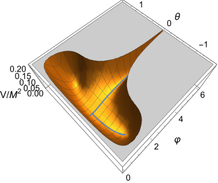
The scalar potential depending upon both fields $\varphi$ and $\theta$, the inflationary trajectory, and the time evolution of both fields in that potential are shown in Fig. 8. We also derived the Hubble function and the slow-roll parameters $\epsilon$ and $\eta$ in the representative model, which are shown in Fig. 9. The initial conditions are the same: $\varphi(0)=6$, $\theta(0)=1.0\times 10^{-4}$ and the vanishing initial velocities.

As is clear from Fig. 8, inflation begins as the single-field slow-roll Starobinsky inflation with $\varphi$ as the inflaton (the first stage of double inflation). When the inflationary trajectory approaches the saddle point where one of the scalars gets a negative mass squared (the signal of tachyonic instability), the inflationary trajectory sharply changes its direction. After that inflation is driven by $\theta$-field as the inflaton (the second stage of double inflation).

As is clear from Fig. 9, there is double inflation indeed because of two plateaus in the profile of the Hubble function, while the slow-roll parameter $\epsilon$ becomes very small, which indicates the presence of the very short ultra-slow-roll phase between the two slow-roll stages. The slow-roll conditions are violated in the ultra-slow-roll regime.

We define the start of the second stage of inflation (or the end of the first stage of inflation) by the time when the parameter $\eta$ first approaches one (or when the parameter $\epsilon$ first reaches its maximum), and the end of the second stage as the time when the parameter $\epsilon$ again reaches one first. The duration of the second stage of the inflation $\Delta N_{2}$ appears to be approximately 22.24 e-folds.

The main (CMB) inflationary observables are given by the spectral index $n_{s}$ and tensor-to-scalar ratio $r$ of scalar and tensor perturbations, respectively. We derived them in order to confront our model against Planck observational results.

The slow-roll parameters $\epsilon$ and $\eta_{\Sigma\Sigma}$ are defined by ($\phi^{A}\equiv\{\varphi,\theta\}$)

		$\displaystyle\epsilon\equiv-{{\dot{H}}\over{H^{2}}}~,\quad\eta_{\Sigma\Sigma}\equiv{{\mathcal{M}_{B}^{A}\Sigma_{A}\Sigma^{B}}\over{V}}~~~,$		(41)
		$\displaystyle\Sigma^{A}\equiv{{\dot{\phi}^{A}}\over{|\dot{\phi}|}}~,\quad\mathcal{M}_{B}^{A}\equiv G^{AC}\nabla_{B}\partial_{C}V-\mathrm{R}^{A}_{~CDB}\dot{\phi}^{C}\dot{\phi}^{D}~,$		(42)

in terms of the metric $G_{AC}$ in the scalar field space and its Riemann-Christoffel curvature $\mathrm{R}^{A}_{~CDB}$. The isocuvature parameter is defined by

$\displaystyle\eta_{\Omega\Omega}\equiv{{\mathcal{M}_{B}^{A}\Omega_{A}\Omega^{B}}\over{V}}~,\quad\mathrm{where}\quad\Omega^{A}\equiv{{{\omega}^{A}}\over{|{\omega}|}}~,\quad\omega\equiv\dot{\Sigma^{A}}+\Gamma^{A}_{BC}\Sigma^{B}\dot{\phi}^{C}~.$

(43)

The transfer function are defined by

	$\displaystyle T_{SS}(t_{1},t_{2})\equiv\exp\left[\int_{t_{2}}^{t_{1}}dt^{\prime}\beta(t^{\prime})H(t^{\prime})\right]~,$		(44)
	$\displaystyle T_{RS}(t_{1},t_{2})\equiv 2\int_{t_{2}}^{t_{1}}dt^{\prime}|\omega(t^{\prime})|T_{SS}(t_{1},t_{2})~,$		(45)
	$\displaystyle\mathrm{where}\quad\beta(t)\equiv-2\epsilon+\eta_{\Sigma\Sigma}-\eta_{\Omega\Omega}-{{4|\omega|^{2}}\over{3H^{2}}}~.$		(46)

These equations are enough to compute the observables by applying the Mathematica packages for numerical calculations with the transport method in multi-field models of inflation [23]. In particular, the observables $n_{s}$ and $r$ are given by

$\displaystyle n_{s}=1-6\epsilon+2\eta_{\Sigma\Sigma}\quad{\rm and}\quad r={{16\epsilon}\over{1+T_{RS}^{2}}}~~.$

(47)

The values of the observables in our representative model at the CMB pivot scale, which corresponds to $k_{\rm CMB}=0.05~{\rm Mpc}^{-1}$ (we set 70 e-folds as the duration of the whole double inflation), and the same initial values mentioned above are shown in Table 1 together with the values of $g_{0}$, the values of $\varphi$ and $\theta$ at the minimum, and the number of e-folds for the second stage of inflation. Table 1 also contains the values of the other parameters, $g_{1}$ and $g_{2}$.

The improved precision measurements of the CMB radiation [5, 6] give for the spectral tilt $n_{s}$ of scalar perturbations the values

$$n_{s}=0.9649\pm 0.0042\quad(68\%~{\rm C.L.})$$

(48)

The current observational upper bound [5, 6] on the CMB tensor-to-scalar ratio $r$ is given by

$$r<0.036\quad(95\%~{\rm C.L.})$$

(49)

As is clear from Table 1, the values of $r$ in our model are well below the observational bound but the values of $n_{s}$ are outside the $1\sigma$ range for the given values of $\Delta N_{2}$, except the case of $g_{1}=-0.25$. The reason for that is our intension to maximize the value of $\Delta N_{2}$ which is crucial for larger PBH masses, see Eq. (51) below. The $1\sigma$ agreement can be achieved by changing the parameters at the expense of decreasing $\Delta N_{2}$ to 10. ³³ 3 For instance, it can be easily achieved by changing the value of $g_{2}$. Nevertheless, it also follows from Table 1 that the $3\sigma$ agreement with the observed value of $n_{s}$ is still possible for $\Delta N_{2}\leq 22.24$.

We found difficult to derive the power spectrum in our models due to field oscillations along $\theta=0$ because our numerical calculations failed. This ”primordial feature” is likely caused due to resonances during inflation on sub-horizon scales. Such resonances can occur when a massive scalar field oscillates at the bottom of the potential [24, 25, 26], like in our model. To avoid this problem, we computed the power spectrum in our model by considering the first and second stages of double inflation separately, see the next Sections. However, it required setting initial conditions at the beginning of the second stage of inflation, which we did not determine and, hence, took them randomly.

In this Section, we take a closer look on dependence of the observables upon initial conditions. There are two independent sets of initial conditions for sinflaton $\theta$ and inflaton $\varphi$. In the Starobinsky-like inflation, the power spectrum is more sensitive to initial conditions on $\theta$ rather than those on $\varphi$ because we deal with the attractor model of inflation where the dependence upon the inflaton initial conditions is suppressed (besides duration of inflation). Our numerical calculations confirm this expectation. That is why we focus on dependence upon initial conditions on $\theta$ and field dynamics near the critical point.

As regards the primordial power spectrum, see the next Section, it is not affected by initial conditions on adiabatic and isocurvature perturbations. It happens because the power spectrum enhancement is determined by behavior of field perturbations near the critical point that is independent upon initial conditions. The evolution of perturbations, obtained by numerical calculations in our model, appears to be usual (as expected) after integrating the equations governing adiabatic and isocurvature perturbations with the isocurvature pumping mechanism, as was described e.g., in Ref. [12], Sections VI and VII.

In order to get the dependence upon the initial value of $\theta$, we numerically computed the duration ($\Delta N_{2}$) of the second stage of inflation (in e-folds) in the representative model for the different values of $\theta(0)$ between $10^{-8}$ and $10^{-2}$. Our numerical results are shown in Fig. 10. As is clear from Fig. 10, the values of $\Delta N_{2}$ weakly depend upon small changes in the initial value of $\theta$. The values of $\Delta N_{2}$ vary from about $20$ to $30$ that changes the corresponding values of the observables by the order of $10^{-2}$. The similar results for the CMB observables are given in Fig. 11, which are a bit more sensitive to initial conditions.

The $\theta$-field is strongly suppressed at its minimum during the first stage of the inflation but becomes sensitive to any additional small impact at the saddle point where quantum corrections (for example, due to quantum diffusion [27]) may become important while the impact of initial conditions becomes negligible. Therefore, we study the first and second stages of inflation separately, and assume a small non-vanishing value (kick) of the $\theta$-velocity at the beginning of the second stage of inflation. We denote $t_{1}$ to be the time at the end of the first stage inflation, and $t_{2}$ to be the time of the end of the second stage of inflation. As regards the first stage of inflation, we use our representative model studied in the preceding Sections with the same initial value for $\varphi$ in order to get the resulting values of $\varphi(t)$ and $\theta(t)$ and their velocities at the end of the first stage of inflation.

Next, we check whether we can get enough e-folds $\Delta N_{2}$ by adding a small $\theta$-velocity at the saddle point. In our representative model we use the parameters $(g_{0},g_{1},g_{2})=(1.1496,-1.0,1.9)$ and the initial values $(\varphi(0),\theta(0))=(6,0)$ with the vanishing initial velocities. Then the values of $\varphi(t)$ and $\varphi^{\prime}(t)$ at the saddle point are $|\varphi(t)|\sim 0.86$ and $\varphi^{\prime}(t)\lesssim\mathcal{O}(0.1)$, respectively. Our result for the dependence of $\Delta N_{2}$ upon the kick velocity $\theta^{\prime}(t_{1})$ at the saddle point is shown in Fig. 12. As is clear from Fig. 12, $\Delta N_{2}\sim 20$ can be achieved with $\theta^{\prime}(t_{1})\sim\mathcal{O}(10^{-10})$.

Having obtained those results, we derived the corresponding CMB observables (with the total duration of inflation given by 70 e-folds) as follows:

$\displaystyle n_{s}=0.9634~,\quad r=0.0038~.$

(50)

In this Section we numerically compute the power spectrum of scalar (curvature) perturbations by using the transport method with the Mathematica package [23] that was widely used in the literature. In order to efficiently produce the primordial black holes, the enhancement (peak) in the power spectrum against its CMB value should be $10^{6}$ times at least. We do not provide here the underlying equations, defining the power spectrum and the ”isocurvature pumping” amplification mechanism, because they are available in the literature, see e.g., subsection III.B of Ref. [12] for details.

Given a peak, the masses of generated PBHs can be calculated by the equation [28]

$\displaystyle M_{\mathrm{PBH}}\simeq{{M_{\mathrm{Pl}}^{2}}\over{H(t_{*})}}\mathrm{exp}\left[2(N_{\mathrm{end}}-N_{*})+\int_{t_{*}}^{t_{\mathrm{exit}}}\epsilon(t)H(t)dt\right]~,$

(51)

where $t_{*}$ and $N_{*}$ are the time and e-folds at the end of the first stage of the inflation, $N_{\mathrm{end}}$ is the number of e-folds at the end of (the second stage) of inflation, and $t_{\mathrm{exit}}$ is the time when the CMB pivot scale exits the horizon. Equation (51) was derived in Ref. [28] by estimating the PBH mass inside the horizon, when the mode corresponding to the peak in the power spectrum re-entered the horizon. As is clear from Eq. (51), the PBH masses are very sensitive to the value of $\Delta N_{2}=(N_{\mathrm{end}}-N_{*})$.

Our first example is the case with $g_{1}=1.0,g_{2}=1.9$, where we have scanned the values of the $\theta$-velocity at the saddle point from $10^{-3}$ to $10^{-6}$. The power spectrum is shown in Fig. 13. As is clear from Fig. 13, the enhancement of the power spectrum strongly depends on the value of $\theta^{\prime}(t_{1})$. In order to get the desired height of the peak from the CMB value of $10^{-9}$ to $10^{-2}$, we have to choose the value of $\theta^{\prime}(t_{1})$ within a small margin. We also give the corresponding PBH masses (in grams) in Fig. 13.

As another example, we choose $g_{1}={-1.0,-0.5,-0.25}$ and adjust the proper values for $g_{2}$ and $g_{0}$. The $\theta^{\prime}(t_{1})$ is chosen to get a peak up to $10^{-2}$ in the power spectrum. The resulting power spectrum is given in Fig. 14.

The parameter values together with the values of the related observables corresponding to Fig. 14 is collected in Table 2. As is clear from Table 2, smaller values of $\left|g_{1}\right|$ lead to larger PBHs masses.

To the end of this Section, we comment on the quadratic Ansatz for the $\tilde{g}$-function in Eq. (2) as

$$\tilde{g}(Z)=M(\tilde{g}_{0}+\tilde{g}_{1}Z+\tilde{g}_{2}Z^{2})$$

(52)

in our search for proper values of its three parameters for double inflation.

We did not find the desired shape of the potential that would support double inflation in this case. To examine the potential, we have set a space with the three parameters $\tilde{g}_{0}$, $\tilde{g}_{1}$ and $\tilde{g}_{2}$ within the range from $-100$ to $+100$, and have imposed the following conditions on the potential: (i) the value of the potential must be positive, (ii) the duration of inflation should be long enough, (iii) the potential along the $\theta$-direction should be stable during the first stage of inflation, and (iv) the height of the potential should be limited from above. By demanding these conditions on the parameter space, no area was found to satisfy them. Therefore, the model with the $\tilde{g}$-function (52) is ruled out. It is worth noticing that the four conditions above are rather mild, e.g., in the case of the quadratic $g$-function they are easily satisfied.

It follows from Table 2 that perfect consistency of our models with CMB measurements restricts the possible PBH masses by $10^{14}$ g even after fine-tuning of the parameters, which is below the Hawking (quantum black hole) evaporation limit of $10^{15}$ g. It means that those PBH cannot be part of the current dark matter.

This in contrast to the different extensions of Starobinsky model in supergravity proposed and investigated in Refs. [13, 16, 29] where the generated PBH masses can reach $10^{21}$ g. It is also different from the non-supersymmetric Appleby-Battye-Starobinsky model [30] adapted in Ref. [31] for PBH production, where the PBH masses can reach $10^{19}$ g.

Of course, all the above goes under the assumption that the PBH do not get extra mass over time during the evolution of the Universe. It might be possible that inflation generates a lot of PBH with masses of $10^{14}$ g, which keep their masses and may get even larger masses via accretion and mergers. However, then one would need a lot of those PBH in order to account for a significant part of the current dark matter, which would contradict to the non-detection of extra-galactic gamma-rays from their Hawking radiation.

We conclude that our supergravity models studied in this paper are consistent with CMB measurements and do lead to the efficient PBH production with the fine-tuned quadratic $g$-function in the superpotential, but those PBH cannot be part of the current dark matter. We did not study more complicated $g$- and $\tilde{g}$-functions beyond quadratic polynomials and exponentials, because it could only be done on the case-by-case basis and would require a separate investigation. In the case of quadratic $g$-functions, which was in the focus of this investigation, all the parameters had to be fixed in order to achieve the desired enhancement of the scalar power spectrum needed for PBH production. The obvious next step would be adding one extra parameter by studying cubic $g(Z)$-functions (our work in progress).

SA was supported by Chung-Ang University and the Basic Science Research Program through the National Research Foundation (NRF) funded by the Ministry of Education, Science and Technology in South Korea under the grant No. NRF-2022R1A2C2003567. RI and SVK were supported by Tokyo Metropolitan University. SVK was also supported by the World Premier International Research Center Initiative (WPI Initiative), MEXT, Japan, the Japanese Society for Promotion of Science under the grant No. 22K03624, and the Tomsk Polytechnic University Development Program Priority-2030-NIP/EB-004-0000-2022.

The authors are grateful to David I. Kaiser, Edward W. Kolb, Burt Ovrut, Misao Sasaki and two anonymous referees for discussions and correspondence.

References

- [1] M. Galante, R. Kallosh, A. Linde, and D. Roest, “Unity of Cosmological Inflation Attractors,” Phys. Rev. Lett. 114 no. 14, (2015) 141302, arXiv:1412.3797 [hep-th].
- [2] T. Terada, “Generalized Pole Inflation: Hilltop, Natural, and Chaotic Inflationary Attractors,” Phys. Lett. B 760 (2016) 674–680, arXiv:1602.07867 [hep-th].
- [3] R. Kallosh and A. Linde, “Polynomial -attractors,” JCAP 04 no. 04, (2022) 017, arXiv:2202.06492 [astro-ph.CO].
- [4] A. A. Starobinsky, “A new type of isotropic cosmological models without singularity,” Phys. Lett. B 91 no. 1, (1980) 99 – 102.
- [5] BICEP, Keck Collaboration, P. A. R. Ade et al., “Improved Constraints on Primordial Gravitational Waves using Planck, WMAP, and BICEP/Keck Observations through the 2018 Observing Season,” Phys. Rev. Lett. 127 no. 15, (2021) 151301, arXiv:2110.00483 [astro-ph.CO].
- [6] M. Tristram et al., “Improved limits on the tensor-to-scalar ratio using BICEP and Planck data,” Phys. Rev. D 105 no. 8, (2022) 083524, arXiv:2112.07961 [astro-ph.CO].
- [7] S. V. Ketov and A. A. Starobinsky, “Embedding -Inflation into Supergravity,” Phys. Rev. D 83 (2011) 063512, arXiv:1011.0240 [hep-th].
- [8] S. V. Ketov, “Supergravity and Early Universe: the Meeting Point of Cosmology and High-Energy Physics,” Int. J. Mod. Phys. A 28 (2013) 1330021, arXiv:1201.2239 [hep-th].
- [9] S. V. Ketov, “On the equivalence of Starobinsky and Higgs inflationary models in gravity and supergravity,” J. Phys. A 53 no. 8, (2020) 084001, arXiv:1911.01008 [hep-th].
- [10] J. Ellis, D. V. Nanopoulos, and K. A. Olive, “No-Scale Supergravity Realization of the Starobinsky Model of Inflation,” Phys. Rev. Lett. 111 (2013) 111301, arXiv:1305.1247 [hep-th]. [Erratum: Phys.Rev.Lett. 111, 129902 (2013)].
- [11] S. Cecotti and R. Kallosh, “Cosmological Attractor Models and Higher Curvature Supergravity,” JHEP 05 (2014) 114, arXiv:1403.2932 [hep-th].
- [12] A. Gundhi, S. V. Ketov, and C. F. Steinwachs, “Primordial black hole dark matter in dilaton-extended two-field Starobinsky inflation,” Phys. Rev. D 103 no. 8, (2021) 083518, arXiv:2011.05999 [hep-th].
- [13] Y. Aldabergenov, A. Addazi, and S. V. Ketov, “Primordial black holes from modified supergravity,” Eur. Phys. J. C 80 no. 10, (2020) 917, arXiv:2006.16641 [hep-th].
- [14] S. V. Ketov, “Multi-Field versus Single-Field in the Supergravity Models of Inflation and Primordial Black Holes,” Universe 7 no. 5, (2021) 115.
- [15] S. R. Geller, W. Qin, E. McDonough, and D. I. Kaiser, “Primordial black holes from multifield inflation with nonminimal couplings,” Phys. Rev. D 106 no. 6, (2022) 063535, arXiv:2205.04471 [hep-th].
- [16] Y. Aldabergenov, A. Addazi, and S. V. Ketov, “Inflation, SUSY breaking, and primordial black holes in modified supergravity coupled to chiral matter,” Eur. Phys. J. C 82 no. 8, (2022) 681, arXiv:2206.02601 [astro-ph.CO].
- [17] V. R. Ivanov, S. V. Ketov, E. O. Pozdeeva, and S. Y. Vernov, “Analytic extensions of Starobinsky model of inflation,” JCAP 03 no. 03, (2022) 058, arXiv:2111.09058 [gr-qc].
- [18] R. Kallosh and A. Linde, “Universality Class in Conformal Inflation,” JCAP 07 (2013) 002, arXiv:1306.5220 [hep-th].
- [19] M. Kawasaki, M. Yamaguchi, and T. Yanagida, “Natural chaotic inflation in supergravity,” Phys. Rev. Lett. 85 (2000) 3572–3575, arXiv:hep-ph/0004243.
- [20] S. Cecotti, “Higher derivative supergravity is equivalent to standard supergravity coupled to matter. 1.,” Phys. Lett. B 190 (1987) 86–92.
- [21] S. J. Gates, Jr. and S. V. Ketov, “Superstring-inspired supergravity as the universal source of inflation and quintessence,” Phys. Lett. B 674 (2009) 59–63, arXiv:0901.2467 [hep-th].
- [22] S. V. Ketov, Quantum nonlinear sigma models: From quantum field theory to supersymmetry, conformal field theory, black holes and strings. Springer-Verlag, 2000.
- [23] M. Dias, J. Frazer, and D. Seery, “Computing observables in curved multifield models of inflation—A guide (with code) to the transport method,” JCAP 12 (2015) 030, arXiv:1502.03125 [astro-ph.CO].
- [24] C. Pahud, M. Kamionkowski, and A. R. Liddle, “Oscillations in the inflaton potential?,” Phys. Rev. D 79 (2009) 083503, arXiv:0807.0322 [astro-ph].
- [25] J. Chluba, J. Hamann, and S. P. Patil, “Features and New Physical Scales in Primordial Observables: Theory and Observation,” Int. J. Mod. Phys. D 24 no. 10, (2015) 1530023, arXiv:1505.01834 [astro-ph.CO].
- [26] J. Fumagalli, S. e. Renaux-Petel, and L. T. Witkowski, “Resonant features in the stochastic gravitational wave background,” JCAP 08 (2021) 059, arXiv:2105.06481 [astro-ph.CO].
- [27] C. Pattison, V. Vennin, D. Wands, and H. Assadullahi, “Ultra-slow-roll inflation with quantum diffusion,” JCAP 04 (2021) 080, arXiv:2101.05741 [astro-ph.CO].
- [28] S. Pi, Y.-l. Zhang, Q.-G. Huang, and M. Sasaki, “Scalaron from -gravity as a heavy field,” JCAP 05 (2018) 042, arXiv:1712.09896 [astro-ph.CO].
- [29] Y. Aldabergenov, A. Addazi, and S. V. Ketov, “Testing Primordial Black Holes as Dark Matter in Supergravity from Gravitational Waves,” Phys. Lett. B 814 (2021) 136069, arXiv:2008.10476 [hep-th].
- [30] S. A. Appleby, R. A. Battye, and A. A. Starobinsky, “Curing singularities in cosmological evolution of F(R) gravity,” JCAP 06 (2010) 005, arXiv:0909.1737 [astro-ph.CO].
- [31] D. Frolovsky, S. V. Ketov, and S. Saburov, “Formation of primordial black holes after Starobinsky inflation,” Mod. Phys. Lett. A 37 no. 21, (2022) 2250135, arXiv:2205.00603 [astro-ph.CO].
- [32] S. Kachru, R. Kallosh, A. D. Linde, and S. P. Trivedi, “De Sitter vacua in string theory,” Phys. Rev. D 68 (2003) 046005, arXiv:hep-th/0301240.