Single-Carrier Delay Alignment Modulation for Multi-IRS Aided Communication

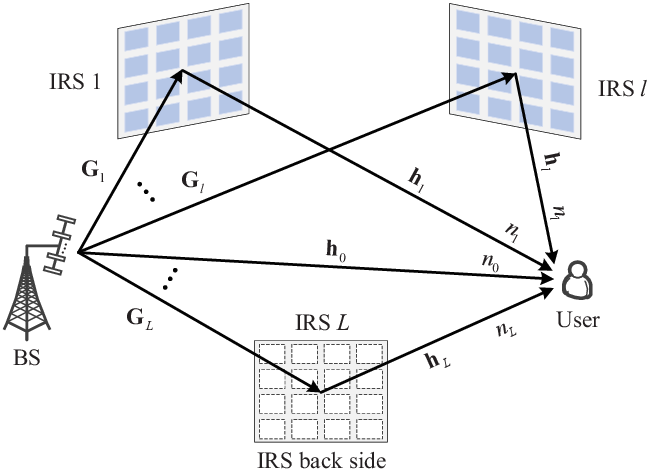
As shown in Fig. 1, we consider a multi-IRS aided wideband communication system, where $L$ IRSs are deployed to assist in the communication from a BS to a user. The BS is equipped with $N_{t}$ antennas, and the user has one antenna. Each IRS consists of $M={M_{h}}{M_{v}}$ passive reflecting elements, where ${M_{h}}$ and ${M_{v}}$ denote the number of elements in the horizontal and vertical dimensions, respectively. Denote by ${{\bf{\Theta}}_{l}}={\rm{diag}}\left({{e^{j{\theta_{l,1}}}},\cdots,{e^{j{\theta_{l,m}}}},\cdots,{e^{j{\theta_{l,M}}}}}\right)$ the diagonal phase-shift matrix of IRS $l$, where ${\theta_{l,m}}\in\left[{0,2\pi}\right)$ is the phase shift of the $m$th reflecting element of IRS $l$, with $m={1,\cdots,M}$ and $l={1,\cdots,L}$. The direct channel from the BS to the user without the reflection by any IRS is denoted by ${\bf{h}}_{0}^{H}\in{{\mathbb{C}}^{1\times{N_{t}}}}$. Let ${{\bf{G}}_{l}}\in{{\mathbb{C}}^{M\times{N_{t}}}}$ denote the channel matrix from the BS to IRS $l$, and ${\bf{h}}_{l}^{H}\in{{\mathbb{C}}^{1\times M}}$ denote the channel vector from IRS $l$ to the user. We focus on the time-dispersive multi-path fading channel between the BS and the user induced by multiple IRSs, where the strongest channel tap is considered for each pair of nodes. Such a time-dispersive channel model is practically valid due to the following reasons. On one hand, for high-frequency systems such as mmWave communications, the effect of LoS component typically dominates since the high frequency signals usually suffer from severe scattering and diffraction losses [4]. As such, the strongest direct channel tap between the BS and the user is considered. On the other hand, to fully exploit the benefits of IRSs, it is desirable to deploy them in LoS conditions with the BS/user [29]. Moreover, the signals experiencing more than one reflection are ignored since they are typically much weaker than those with one reflection only [38, 49]. We assume quasi-static block fading model, where the channel remains unchanged within each channel coherence interval. The discrete-time equivalent of the channel impulse response from the BS to the user can be expressed as

where $n_{0}$ denotes the discrete-time delay of the direct channel, and $n_{l}$ denotes the delay of the reflected channel via IRS $l$. For ease of exposition, we assume that different IRSs create multi-paths with different resolvable delays, i.e., ${n_{l}}\neq{n_{l^{\prime}}}$, $\forall l\neq l^{\prime}$. Let ${n_{\min}}\triangleq\mathop{\min}\limits_{0\leq l\leq L}{n_{l}}$ and ${n_{\max}}\triangleq\mathop{\max}\limits_{0\leq l\leq L}{n_{l}}$ be the minimum and maximum delay over all the $L+1$ multi-paths, respectively. Then the channel delay spread is defined as ${n_{\rm{span}}}\triangleq{n_{\max}}-{n_{\min}}$. To reveal the fundamental performance limit achieved by DAM, we assume that perfect CSI is available at the BS. In particular, the CSI acquisition of the individual path information, e.g., angle of arrival/departure (AoA/AoD) and propagation delay will become more feasible with the use of large antenna arrays at the BS [2, 3] and the trend of integrated sensing and communication (ISAC) [22, 51]. A preliminary study on CSI acquisition for DAM is being pursued in another parallel work [10], and the channel estimation for the considered multi-IRS system requires more in-depth studies in the future.

Denote by ${\bf{x}}\left[n\right]\in{{\mathbb{C}}^{{N_{t}}\times 1}}$ the discrete-time equivalent of the transmitted signal. Then the received signal is

where $z\left[n\right]\sim{\cal CN}\left({0,{\sigma^{2}}}\right)$ is the AWGN.

Before introducing the DAM transmission and providing its asymptotic performance analysis for multi-IRS aided wideband communication, we first investigate the correlation of the channels associated with the $L+1$ multi-paths. For ease of illustration, we assume here the LoS-dominating channel between the BS and each IRS $l$, and denote by ${\varphi_{l}}$ and ${\phi_{l}}$ the AoD and AoA from the BS to IRS $l$, respectively. The channel matrix ${\bf{G}}_{l}$ is then expressed as ${{\bf{G}}_{l}}={\alpha_{l}}{{\bf{a}}_{R}}\left({{\phi_{l}}}\right){\bf{a}}_{T}^{H}\left({{\varphi_{l}}}\right)$, where ${\alpha_{l}}$ is the complex-valued path gain, and ${{\bf{a}}_{R}}\left({{\phi_{l}}}\right)\in{{\mathbb{C}}^{M\times 1}}$ and ${{\bf{a}}_{T}}\left({{\varphi_{l}}}\right)\in{{\mathbb{C}}^{{N_{t}}\times 1}}$ denote the receive and transmit array response vectors, respectively. If the BS is equipped with the basic uniform linear array (ULA) with adjacent elements separated by half wavelength, the transmit array response vector can be expressed as [52]

Similarly, the direct channel ${\bf h}_{0}$ can be expressed as ${{\bf{h}}_{0}}={\alpha_{0}}{{\bf{a}}_{T}}\left({{\varphi_{0}}}\right)$, where ${\alpha_{0}}$ is the complex coefficient of the direct channel, and ${{\varphi_{0}}}$ is its AoD. It then follows from [9] that as long as the $L$ IRSs and the direct link are associated with distinct AoDs, the corresponding transmit array response vectors tend to be asymptotically orthogonal when ${N_{t}}\gg L$, i.e.,

Furthermore, since ${{\bf{G}}_{l}}={\alpha_{l}}{{\bf{a}}_{R}}\left({{\phi_{l}}}\right){\bf{a}}_{T}^{H}\left({{\varphi_{l}}}\right)$, based on (4), we have

As discussed in [9] and further elaborated in Section II-B, such a property motivates our proposed DAM technique as a new solution for ISI-free communication, without relying on sophisticated channel equalization or multi-carrier transmission.

With single-carrier DAM, the signal transmitted by the BS is [1, 9]

where $s\left[n\right]$ is the independent and identically distributed (i.i.d.) information-bearing symbol with zero mean and unit variance, ${\bf{f}}_{l^{\prime}}\in{{\mathbb{C}}^{{N_{t}}\times 1}}$ denotes the path-based transmit beamforming vector associated with path $l^{\prime}$, and $\kappa_{l^{\prime}}\geq 0$ is the deliberately introduced delay pre-compensation for the symbol sequence $s\left[n\right]$, with ${\kappa_{l}}\neq{\kappa_{l^{\prime}}}$, $\forall l\neq l^{\prime}$. The transmit power of the BS is

where $P$ denotes the available transmit power, and the first equality holds since $s\left[n\right]$ is independent across different $n$ and ${\kappa_{l}}\neq{\kappa_{l^{\prime}}}$, $\forall l\neq l^{\prime}$. By substituting (7) into (2), the signal received by the user can be expressed as

By letting ${\kappa_{l^{\prime}}}={n_{\max}}-{n_{l^{\prime}}}\geq 0$, $\forall l^{\prime}\in\left[0,L\right]$, we have

where we have used the equation ${\bf{h}}_{l}^{H}{{\bf{\Theta}}_{l}}{{\bf{G}}_{l}}={\bf{v}}_{l}^{H}{\rm{diag}}\left({{\bf{h}}_{l}^{H}}\right){{\bf{G}}_{l}}$, with ${{\bf{v}}_{l}}={\left[{{e^{j{\theta_{l,1}}}},\cdots,{e^{j{\theta_{l,M}}}}}\right]^{H}}$. It is observed from (10) that if the user is locked to the delay $n_{\max}$, then the first term contributes to the desired signal, while the second and the third terms are the detrimental ISI.

Fortunately, for massive MIMO system with ${N_{t}}\gg L$, we will show that the ISI term in (10) vanishes with the simple path-based MRT beamforming, thanks to the asymptotically orthogonal properties (4)-(6). With path-based MRT beamforming, each beamforming vector ${{\bf{f}}_{l^{\prime}}}$ in (7) matches the transmit array response vector of the corresponding multi-path, which is given by

where $p_{l^{\prime}}$ denotes the power allocation for the $l^{\prime}$th multi-path. By substituting (11) into (10), and after scaling the received signal $y\left[n\right]$ by $1/\sqrt{{N_{t}}}$, we have (12), shown at the top of the next page, where we have used the asymptotical property (4).

By multiplying (12) with $\sqrt{{N_{t}}}$, the signal in (10) reduces to

It is observed from (10) and (13) that thanks to the asymptotical orthogonal properties (4)-(6), the ISI terms in (10) vanish almost surely with the proposed DAM transmission using delay pre-compensation and the simple path-based MRT beamforming. Therefore, the original time-dispersive channel has been transformed to an ISI-free AWGN channel, while still benefiting from the multiplicative gain contributed by all the $L+1$ multi-path signal components. Also, this is free from the sophisticated channel equalization or multi-carrier transmission. Note that similar derivation and conclusion have been made in [9] for DAM communication without IRS. The SNR of (13) is then given by

It is not difficult to see that to maximize the SNR in (14), the phase shift vectors ${\bf{v}}_{l}$ should be designed so that $\arg\left({\alpha_{0}^{*}}\right)=\arg\left({{\alpha_{l}}{\bf{v}}_{l}^{H}{\rm{diag}}\left({{\bf{h}}_{l}^{H}}\right){{\bf{a}}_{R}}\left({{\phi_{l}}}\right)}\right)$, $\forall l$, which yields

By substituting (15) into (14), the resulting SNR is

where ${h}_{l,m}^{*}$ and ${{a}_{R,m}}\left({{\phi_{l}}}\right)$ are the $m$th element of ${{\bf{h}}_{l}^{H}}$ and ${{\bf{a}}_{R}}\left({{\phi_{l}}}\right)$, respectively, and we have used the property that the receive array response vector ${{\bf{a}}_{R}}\left({{\phi_{l}}}\right)$ has unit modulus for each element, i.e., $\left|{{a_{R,m}}\left({{\phi_{l}}}\right)}\right|=1$. By considering the transmit power constraint in (8), the optimal power allocation to maximize the SNR in (16) can be obtained based on the Cauchy-Schwarz inequality, which is given by

The resulting SNR is

where ${\bar{P}}\triangleq P/{\sigma^{2}}$.

As a side result, the closed-form expression (18) is quite useful to compare the centralized versus distributed IRS deployment strategies, by fixing the total number of reflecting elements to $LM$. For ease of elaboration, we consider the LoS-dominating channels between each IRS and the user, for which ${{\bf{h}}_{l}}$ can be modelled as

where ${\beta_{l}}$ denotes the complex-valued path gain, $\bar{d}$ denotes the inter-element spacing normalized by signal wavelength, and ${\vartheta_{l,e}}$ and ${\vartheta_{l,a}}$ denote the corresponding elevation and azimuth AoDs, respectively. In this case, $\left|{{h_{l,m}}}\right|=\left|{{\beta_{l}}}\right|$, $\forall m$, and ${\left\|{{{\bf{h}}_{l}}}\right\|_{1}}=M\left|{{\beta_{l}}}\right|$. Therefore, the SNR in (18) reduces to

where ${l_{\max}}=\arg\mathop{\max}\limits_{1\leq l\leq L}{\left|{{\alpha_{l}}{\beta_{l}}}\right|^{2}}$. It is observed from (20) that for the distributed IRS deployment with a total of $LM$ reflecting elements, the received SNR scales with $L{M^{2}}$, rather than ${\left({LM}\right)^{2}}$ as for centralized deployment [38]. It is worth remarking that although the above result is derived for DAM time-dispersive communications, it is also applicable for narrowband systems as considered in [38]. By substituting $M$ with $LM$ and $L$ with 1 in (20), we get the SNR result for centralized IRS deployment, i.e., one single IRS with $LM$ reflecting elements, given by

It then follows from (20) and (21) that when the centralized IRS is placed at the strongest path, i.e., $l_{\max}=1$, we have $\gamma_{\rm distributed}\leq{\gamma_{{\rm{centralized}}}}$. This is expected since for centralized IRS deployment, the BS only needs to concentrate its power towards one single direction, whereas it needs to split its power towards multiple IRSs for distributed IRS deployment. However, one should not make the simple conclusion that centralized IRS is always superior to distributed one, since the above result is obtained based on the asymptotic analysis and only single-user scenario is considered. For multi-user or multi-cell scenarios, it is quite likely that distributed IRS deployment is necessary due to its higher macro-diversity than centralized deployment.

The above asymptotic analysis with ${N_{t}}\gg L$ shows the capability of DAM to transform the time-dispersive channel to ISI-free AWGN channel with the simple path-based MRT beamforming and delay pre-compensation, which provides an important insight for applying the low-complexity DAM to address the ISI issue in large antenna array systems. In the following, we study the DAM design for the general case with finite $N_{t}$ and $L$, when the orthogonal properties in (4)-(6) do not hold. In this case, the three standard beamforming design approaches, namely ZF, MMSE, and MRT, are studied, on the per-path basis tailored for DAM transmission.

For any given IRS phase shift vectors $\left\{{{\bf{v}}_{l}}\right\}_{l=1}^{L}$, the sub-problem of (P-ZF) for optimizing the beamforming vectors $\left\{{{{\bf{f}}_{l^{\prime}}}}\right\}_{l^{\prime}=0}^{L}$ can be written as

where ${\bf{\tilde{h}}}_{0}^{H}$ and ${\bf{\tilde{h}}}_{l}^{H}$ are defined below (23).

Let ${\bf{H}}\in{{\mathbb{C}}^{{N_{t}}\times\left({L+1}\right)}}\triangleq[{{{\bf{\tilde{h}}}_{0}},{{{\bf{\tilde{h}}}}_{1}},\cdots,{{{\bf{\tilde{h}}}}_{L}}}]$, and ${\bf{F}}\in{{\mathbb{C}}^{{N_{t}}\times\left({L+1}\right)}}\triangleq\left[{{{\bf{f}}_{0}},{{\bf{f}}_{1}},\cdots,{{\bf{f}}_{L}}}\right]$. Without loss of generality, ${\bf{F}}$ can be decomposed as ${\bf{W}}{{\bf{\Lambda}}^{1/2}}$, where ${\bf{W}}\in{{\mathbb{C}}^{{N_{t}}\times\left({L+1}\right)}}\triangleq\left[{{{\bf{w}}_{0}},{{\bf{w}}_{1}},\cdots,{{\bf{w}}_{L}}}\right]$ is designed to ensure the ZF constraints (22) and (23), and ${\bf{\Lambda}}\triangleq{\rm{diag}}\left({{\mu_{0}},{\mu_{1}},\cdots,{\mu_{L}}}\right)$ contains the power allocation coefficient $\mu_{l^{\prime}}$ so that the total power constraint $\sum\nolimits_{l^{\prime}=0}^{L}{{{\left\|{{{\bf{f}}_{l^{\prime}}}}\right\|}^{2}}}=P$ is satisfied. In the following, we first determine ${\bf{W}}$ by noting that one effective beamforming design that satisfies the ZF constraints (22) and (23) is by ensuring ${{\bf{H}}^{H}}{\bf{W}}={{\bf{I}}_{L+1}}$. With ${N_{t}}\geq L+1$, the matrix ${\bf{W}}$ can be obtained by taking the right pseudo inverse of ${{\bf{H}}^{H}}$, i.e., ${\bf{W}}={({{\bf{H}}^{H}})^{+}}={\bf{H}}{({{\bf{H}}^{H}}{\bf{H}})^{-1}}$. Thus, ${{\bf{f}}_{l^{\prime}}}$ can be expressed as ${{\bf{f}}_{l^{\prime}}}=\sqrt{{\mu_{l^{\prime}}}}{{\bf{w}}_{l^{\prime}}}$, where ${\bf{w}}_{l^{\prime}}$ is the $\left(l^{\prime}+1\right)$th column of ${({{\bf{H}}^{H}})}^{+}$, and the remaining task is to find the optimal power allocation coefficient $\mu_{l^{\prime}}$ by solving the following optimization problem:

where we have used the relationship ${\bf{\tilde{h}}}_{l^{\prime}}^{H}{{\bf{w}}_{l^{\prime}}}=1$ based on the property of pseudo inverse, $\forall l^{\prime}\in\left[0,L\right]$.

For any given beamforming vectors $\left\{{{{\bf{f}}_{l^{\prime}}}}\right\}_{l^{\prime}=0}^{L}$ in (P-ZF), the sub-problem of phase shift optimization is given by

Note that in (P-ZF2), we have expressed the ZF constraint of (P-ZF) by its equivalent quadratic form.

Let ${\bf{\tilde{v}}}\in{{\mathbb{C}}^{\left({LM+1}\right)\times 1}}\triangleq{\left[{{\bf{v}}_{1}^{T},\cdots,{\bf{v}}_{L}^{T},1}\right]^{T}}$, ${\bf{\tilde{f}}}\in{{\mathbb{C}}^{\left({LM+1}\right)\times 1}}$ $\triangleq{[{({\rm{diag}}\left({{\bf{h}}_{1}^{H}}\right){{\bf{G}}_{1}}{{\bf{f}}_{1}})^{T}},\cdots,{({\rm{diag}}\left({{\bf{h}}_{L}^{H}}\right){{\bf{G}}_{L}}{{\bf{f}}_{L}})^{T}},{\bf{h}}_{0}^{H}{{\bf{f}}_{0}}]^{T}}$. Then the objective function of (P-ZF2) can be compactly written as ${|{{{{\bf{\tilde{v}}}}^{H}}{\bf{\tilde{f}}}}|^{2}}/{\sigma^{2}}$. Furthermore, for any $l\in\left[1,L\right]$, define the selection matrix ${{\bf{S}}_{l}}\in{{\mathbb{C}}^{M\times\left({LM+1}\right)}}$ so that ${{\bf{v}}_{l}}={{\bf{S}}_{l}}{\bf{\tilde{v}}}$, which can be obtained by setting the $\left({\left({l-1}\right)M+i}\right)$th element of the $i$th row as one, and the other elements as zero, $\forall i\in\left[1,M\right]$. Therefore, the first constraint of (P-ZF2) can be expressed as ${|{{{{\bf{\tilde{v}}}}^{H}}{{\bf{b}}_{l,l^{\prime}}}}|^{2}}\leq 0$, $\forall l\neq l^{\prime}$, $l\in\left[{1,L}\right]$, $l^{\prime}\in\left[{0,L}\right]$, where ${{\bf{b}}_{l,l^{\prime}}}\in{{\mathbb{C}}^{\left({LM+1}\right)\times 1}}\triangleq{\bf{S}}_{l}^{H}{\rm{diag}}\left({{\bf{h}}_{l}^{H}}\right){{\bf{G}}_{l}}{{\bf{f}}_{l^{\prime}}}$. Then (P-ZF2) can be compactly written as

where ${\tilde{v}}_{m}$ is the $m$th element of ${\bf{\tilde{v}}}$. The objective function of (31) is convex, the maximization of which is a non-convex optimization problem. Fortunately, effective solution can be obtained by successive convex approximation (SCA) technique, which is an efficient iterative algorithm that successively updates the optimization variable at each iteration. Specifically, let ${\bf{\tilde{v}}}_{r}$ be the resulting optimization variable after the $r$th iteration. We have

As a result, problem (31) is lower-bounded by the following problem for any given ${\bf{\tilde{v}}}_{r}$

which is a convex optimization problem and can be efficiently solved by standard convex optimization tools, such as CVX.

The main procedure for solving (P-ZF) is summarized in Algorithm 1, with its convergence shown below.

References

- [1] H. Lu and Y. Zeng, “Delay alignment modulation: Enabling equalization-free single-carrier communication,” IEEE Wireless Commun. Lett., vol. 11, no. 9, pp. 1785–1789, Sep. 2022.
- [2] E. Björnson, L. Sanguinetti, H. Wymeersch, J. Hoydis, and T. L. Marzetta, “Massive MIMO is a reality – what is next?: Five promising research directions for antenna arrays,” Digit. Signal Process., vol. 94, pp. 3–20, Nov. 2019.
- [3] H. Lu and Y. Zeng, “Communicating with extremely large-scale array/surface: Unified modeling and performance analysis,” IEEE Trans. Wireless Commun., vol. 21, no. 6, pp. 4039–4053, Jun. 2022.
- [4] M. R. Akdeniz, Y. Liu, M. K. Samimi, S. Sun, S. Rangan, T. S. Rappaport, and E. Erkip, “Millimeter wave channel modeling and cellular capacity evaluation,” IEEE J. Sel. Areas Commun., vol. 32, no. 6, pp. 1164–1179, Jun. 2014.
- [5] Y. Zeng and R. Zhang, “Millimeter wave MIMO with lens antenna array: A new path division multiplexing paradigm,” IEEE Trans. Commun., vol. 64, no. 4, pp. 1557–1571, Apr. 2016.
- [6] T. S. Rappaport, Y. Xing, O. Kanhere, S. Ju, A. Madanayake, S. Mandal, A. Alkhateeb, and G. C. Trichopoulos, “Wireless communications and applications above 100 GHz: Opportunities and challenges for 6G and beyond,” IEEE Access, vol. 7, pp. 78 729–78 757, Jun. 2019.
- [7] Y. Chen, L. Yan, and C. Han, “Hybrid spherical-and planar-wave modeling and DCNN-powered estimation of terahertz ultra-massive MIMO channels,” IEEE Trans. Commun., vol. 69, no. 10, pp. 7063–7076, Oct. 2021.
- [8] Y. Zeng, L. Yang, and R. Zhang, “Multi-user millimeter wave MIMO with full-dimensional lens antenna array,” IEEE Trans. Wireless Commun., vol. 17, no. 4, pp. 2800–2814, Apr. 2018.
- [9] H. Lu and Y. Zeng, “Delay alignment modulation: Manipulating channel delay spread for efficient single- and multi-carrier communication,” IEEE Trans. Commun., 2023.
- [10] D. Ding and Y. Zeng, “Channel estimation for delay alignment modulation,” arXiv preprint arXiv:2206.09339, 2022.
- [11] Z. Xiao and Y. Zeng, “Integrated sensing and communication with delay alignment modulation: Performance analysis and beamforming optimization,” IEEE Trans. Wireless Commun., 2023, DOI: 10.1109/TWC.2023.3266758.
- [12] P. J. Melsa, R. C. Younce, and C. E. Rohrs, “Impulse response shortening for discrete multitone transceivers,” IEEE Trans. Commun., vol. 44, no. 12, pp. 1662–1672, Dec. 1996.
- [13] R. K. Martin, K. Vanbleu, M. Ding, G. Ysebaert, M. Milosevic, B. L. Evans, M. Moonen, and C. R. Johnson, “Unification and evaluation of equalization structures and design algorithms for discrete multitone modulation systems,” IEEE Trans. Signal Process., vol. 53, no. 10, pp. 3880–3894, Oct. 2005.
- [14] M. Emami, M. Vu, J. Hansen, A. J. Paulraj, and G. Papanicolaou, “Matched filtering with rate back-off for low complexity communications in very large delay spread channels,” in Proc. 38th Asilomar Conf. Signals, Syst. Comput., vol. 1, 2004, pp. 218–222.
- [15] F. Han, Y.-H. Yang, B. Wang, Y. Wu, and K. R. Liu, “Time-reversal division multiple access over multi-path channels,” IEEE Trans. Commun., vol. 60, no. 7, pp. 1953–1965, Jul. 2012.
- [16] Y. Chen, B. Wang, Y. Han, H.-Q. Lai, Z. Safar, and K. R. Liu, “Why time reversal for future 5G wireless? [perspectives],” IEEE Signal Process. Mag., vol. 33, no. 2, pp. 17–26, Mar. 2016.
- [17] A. Pitarokoilis, S. K. Mohammed, and E. G. Larsson, “On the optimality of single-carrier transmission in large-scale antenna systems,” IEEE Wireless Commun. Lett., vol. 1, no. 4, pp. 276–279, Aug. 2012.
- [18] R.-A. Pitaval, “Channel shortening by large multiantenna precoding in OFDM,” IEEE Trans. Commun., vol. 69, no. 5, pp. 2878–2893, May 2021.
- [19] A. Goldsmith, Wireless communications. Cambridge, U.K.: Cambridge Univ. Press, 2005.
- [20] R. W. Heath Jr and A. Lozano, Foundations of MIMO communication. Cambridge, U.K.: Cambridge Univ. Press, 2018.
- [21] S. H. Han and J. H. Lee, “An overview of peak-to-average power ratio reduction techniques for multicarrier transmission,” IEEE Wireless Commun., vol. 12, no. 2, pp. 56–65, Apr. 2005.
- [22] W. Tong and P. Zhu, 6G, the next horizon: From connected people and things to connected intelligence. Cambridge, U.K.: Cambridge Univ. Press, 2021.
- [23] R. Nissel, S. Schwarz, and M. Rupp, “Filter bank multicarrier modulation schemes for future mobile communications,” IEEE J. Sel. Areas Commun., vol. 35, no. 8, pp. 1768–1782, Aug. 2017.
- [24] Y. Yao and G. B. Giannakis, “Blind carrier frequency offset estimation in SISO, MIMO, and multiuser OFDM systems,” IEEE Trans. Commun., vol. 53, no. 1, pp. 173–183, Jan. 2005.
- [25] R. Hadani et al., “Orthogonal time frequency space modulation,” in Proc. IEEE Wireless Commun. Netw. Conf. (WCNC), Mar. 2017, pp. 1–6.
- [26] L. Xiao, S. Li, Y. Qian, D. Chen, and T. Jiang, “An overview of OTFS for Internet of Things: Concepts, benefits and challenges,” IEEE Internet Things J., vol. 9, no. 10, pp. 7596–7618, May 2022.
- [27] T. Taniguchi, H. Hoang, X. N. Tran, and Y. Karasawa, “Maximum SINR design and performance analysis of MIMO communication systems with tapped delay line structure,” in Proc. 15th IEEE Int. Symp. Pers. Indoor Mobile Radio Commun. (PIMRC), 2004, pp. 58–62.
- [28] Q. Wu and R. Zhang, “Towards smart and reconfigurable environment: Intelligent reflecting surface aided wireless network,” IEEE Commun. Mag., vol. 58, no. 1, pp. 106–112, Jan. 2020.
- [29] Q. Wu, S. Zhang, B. Zheng, C. You, and R. Zhang, “Intelligent reflecting surface aided wireless communications: A tutorial,” IEEE Trans. Commun., vol. 69, no. 5, pp. 3313–3351, May 2021.
- [30] E. Basar, M. Di Renzo, J. De Rosny, M. Debbah, M. S. Alouini, and R. Zhang, “Wireless communications through reconfigurable intelligent surfaces,” IEEE Access, vol. 7, pp. 116 753–116 773, Aug. 2019.
- [31] Y. Han, W. Tang, S. Jin, C. Wen, and X. Ma, “Large intelligent surface-assisted wireless communication exploiting statistical CSI,” IEEE Trans. Veh. Technol., vol. 68, no. 8, pp. 8238–8242, Aug. 2019.
- [32] Z.-Q. He and X. Yuan, “Cascaded channel estimation for large intelligent metasurface assisted massive MIMO,” IEEE Wireless Commun. Lett., vol. 9, no. 2, pp. 210–214, Feb. 2020.
- [33] H. Lu, Y. Zeng, S. Jin, and R. Zhang, “Aerial intelligent reflecting surface: Joint placement and passive beamforming design with 3D beam flattening,” IEEE Trans. Wireless Commun., vol. 20, no. 7, pp. 4128–4143, Jul. 2021.
- [34] C. Feng, H. Lu, Y. Zeng, S. Jin, and R. Zhang, “Wireless communication with extremely large-scale intelligent reflecting surface,” in Proc. IEEE/CIC Int. Conf. Commun. Workshops China (ICCC Workshops), Jul. 2021, pp. 165–170.
- [35] M. Di Renzo, A. Zappone, M. Debbah, M.-S. Alouini, C. Yuen, J. de Rosny, and S. Tretyakov, “Smart radio environments empowered by reconfigurable intelligent surfaces: How it works, state of research, and the road ahead,” IEEE J. Sel. Areas Commun., vol. 38, no. 11, pp. 2450–2525, Nov. 2020.
- [36] W. Tang, M. Z. Chen, X. Chen, J. Y. Dai, Y. Han, M. D. Renzo, Y. Zeng, S. Jin, Q. Cheng, and T. J. Cui, “Wireless communications with reconfigurable intelligent surface: Path loss modeling and experimental measurement,” IEEE Trans. Wireless Commun., vol. 20, no. 1, pp. 421–439, Jan. 2021.
- [37] C. Huang, A. Zappone, G. C. Alexandropoulos, M. Debbah, and C. Yuen, “Reconfigurable intelligent surfaces for energy efficiency in wireless communication,” IEEE Trans. Wireless Commun., vol. 18, no. 8, pp. 4157–4170, Aug. 2019.
- [38] Q. Wu and R. Zhang, “Intelligent reflecting surface enhanced wireless network via joint active and passive beamforming,” IEEE Trans. Wireless Commun., vol. 18, no. 11, pp. 5394–5409, Nov. 2019.
- [39] C. Pan et al., “An overview of signal processing techniques for RIS/IRS-aided wireless systems,” IEEE J. Sel. Top. Signal Process., vol. 16, no. 5, pp. 883–917, Aug. 2022.
- [40] X. Shao, C. You, W. Ma, X. Chen, and R. Zhang, “Target sensing with intelligent reflecting surface: Architecture and performance,” IEEE J. Sel. Areas Commun., vol. 40, no. 7, pp. 2070–2084, Mar. 2022.
- [41] Y. Han, S. Zhang, L. Duan, and R. Zhang, “Cooperative double-IRS aided communication: Beamforming design and power scaling,” IEEE Wireless Commun. Lett., vol. 9, no. 8, pp. 1206–1210, Aug. 2020.
- [42] C. You, B. Zheng, and R. Zhang, “Wireless communication via double IRS: Channel estimation and passive beamforming designs,” IEEE Wireless Commun. Lett., vol. 10, no. 2, pp. 431–435, Feb. 2021.
- [43] Y. Gao, J. Xu, W. Xu, D. W. K. Ng, and M.-S. Alouini, “Distributed IRS with statistical passive beamforming for MISO communications,” IEEE Wireless Commun. Lett., vol. 10, no. 2, pp. 221–225, Feb. 2021.
- [44] G. Ding, F. Yang, L. Ding, and Y. Cui, “Analysis and optimization of a double-IRS cooperatively assisted system with a quasi-static phase shift design,” IEEE Trans. Wireless Commun., vol. 22, no. 7, pp. 4416–4433, Jul. 2023.
- [45] Y. Jia, Y. Cui, and W. Jiang, “Robust optimization of instantaneous beamforming and quasi-static phase shifts in an IRS-assisted multi-cell network,” IEEE Trans. Wireless Commun., vol. 21, no. 6, pp. 4394–4409, Jun. 2022.
- [46] Y. Yang, B. Zheng, S. Zhang, and R. Zhang, “Intelligent reflecting surface meets OFDM: Protocol design and rate maximization,” IEEE Trans. Commun., vol. 68, no. 7, pp. 4522–4535, Jul. 2020.
- [47] B. Zheng and R. Zhang, “Intelligent reflecting surface-enhanced OFDM: Channel estimation and reflection optimization,” IEEE Wireless Commun. Lett., vol. 9, no. 4, pp. 518–522, Apr. 2020.
- [48] M. He, W. Xu, H. Shen, G. Xie, C. Zhao, and M. Di Renzo, “Cooperative multi-RIS communications for wideband mmwave MISO-OFDM systems,” IEEE Wireless Commun. Lett., vol. 10, no. 11, pp. 2360–2364, Nov. 2021.
- [49] S. Zhang and R. Zhang, “Capacity characterization for intelligent reflecting surface aided MIMO communication,” IEEE J. Sel. Areas Commun., vol. 38, no. 8, pp. 1823–1838, Aug. 2020.
- [50] H. Li, W. Cai, Y. Liu, M. Li, Q. Liu, and Q. Wu, “Intelligent reflecting surface enhanced wideband MIMO-OFDM communications: From practical model to reflection optimization,” IEEE Trans. Commun., vol. 69, no. 7, pp. 4807–4820, Jul. 2021.
- [51] J. A. Zhang, M. L. Rahman, K. Wu, X. Huang, Y. J. Guo, S. Chen, and J. Yuan, “Enabling joint communication and radar sensing in mobile networks-a survey,” IEEE Commun. Surv. Tut., vol. 24, no. 1, pp. 306–345, First quarter 2022.
- [52] D. Tse and P. Viswanath, Fundamentals of wireless communication. Cambridge, U.K.: Cambridge Univ. Press, 2005.
- [53] F. Sohrabi and W. Yu, “Hybrid digital and analog beamforming design for large-scale antenna arrays,” IEEE J. Sel. Top. Signal Process., vol. 10, no. 3, pp. 501–513, 2016.
- [54] W. Huang, Y. Zeng, and Y. Huang, “Achievable rate region of MISO interference channel aided by intelligent reflecting surface,” IEEE Trans. Veh. Technol., vol. 69, no. 12, pp. 16 264–16 269, Dec. 2020.
- [55] X.-G. Xia, “Precoded and vector OFDM robust to channel spectral nulls and with reduced cyclic prefix length in single transmit antenna systems,” IEEE Trans. Commun., vol. 49, no. 8, pp. 1363–1374, Aug. 2001.