Random Orthogonalization for Federated Learning in Massive MIMO Systems

The FL problem studied in this paper mostly follows that in the original paper [2]. In particular, we consider an FL system with one central parameter server (e.g., base station) and a set of at most $N$ clients (e.g., mobile devices). Client $k\in[N]\triangleq\{1,2,\cdots,N\}$ stores a local dataset $\mathcal{D}_{k}=\{\mathbf{\xi}_{i}\}_{i=1}^{D_{k}}$, with its size denoted by $D_{k}$, that never leaves the client. Datasets across clients are assumed to be non-i.i.d. and disjoint. The maximum data size when all clients participate in FL is $D=\sum_{k=1}^{N}D_{k}$. Each data sample $\mathbf{\xi}$ is denoted by an input-output pair $\{\mathbf{x},y\}$ for a supervised learning task. We use $f_{k}({\bf w})$ to denote the local loss function at client $k$, which measures how well an ML model with parameter ${\bf w}\in\mathbb{R}^{d}$ fits its local dataset. The global objective function over all $N$ clients is $f({\bf w})=\sum_{k\in[N]}p_{k}f_{k}({\bf w}),$ where $p_{k}=\frac{D_{k}}{D}$ is the weight of each local loss function, and the purpose of FL is to distributively find the optimal model parameter ${\bf w}^{*}$ that minimizes the global loss function: ${\bf w}^{*}\triangleq\argmin_{{\bf w}\in\mathbb{R}^{d}}f({\bf w}).$ Let $f^{*}$ and $f_{k}^{*}$ be the minimum value of $f({\bf w})$ and $f_{k}({\bf w})$, respectively. Then, $\Gamma=f^{*}-\sum_{k=1}^{N}\frac{D_{k}}{D}f_{k}^{*}$ quantifies the degree of non-i.i.d. as defined in [16].

Specifically, the FL pipeline [2] iteratively executes the following steps at the $t$-th learning round.

1. 1.

   Downlink communication. The BS broadcasts the current global model ${\bf w}_{t}$ to $K$ randomly selected clients over the downlink wireless channel. We use $[K]$ to denote the selected client set to simplify the notation, but this should be interpreted as possibly different sets of clients at different round $t$.

2. 2.

   Local computation. Each selected client uses its local dataset to train a local model improved upon the received global model ${\bf w}_{t}$. We assume that mini-batch SGD is used to minimize the local loss function. The parameter is updated iteratively (for $E$ steps) at client $k$ as: ${\bf w}_{t,0}^{k}={\bf w}_{t};{\bf w}_{t,\tau}^{k}={\bf w}_{t,\tau-1}^{k}-\eta_{t}\nabla\tilde{f}_{k}({\bf w}_{t,\tau-1}^{k}),\forall\tau=1,\cdots,E;{\bf w}_{t+1}^{k}={\bf w}_{t,E}^{k}$, where $\nabla\tilde{f}_{k}({\bf w})$ denotes the mini-batch SGD operation at client $k$ on model ${\bf w}$, and $\eta_{t}$ is the learning rate (step size).

3. 3.

   Uplink communication. Each selected client uploads its latest local model to the server synchronously over the uplink wireless channel.

4. 4.

   Server aggregation. The BS aggregates the received noisy local models $\tilde{\bf w}_{t+1}^{k}$ to generate a new global model: ${\bf w}_{t+1}=\Sigma_{k\in[K]}\tilde{p}_{k}\tilde{\bf w}_{t+1}^{k}$, where $\tilde{p}_{k}\triangleq\frac{D_{k}}{\Sigma k\in[K]D_{k}}$. For simplicity, we assume that each local dataset has equal size, hence $\tilde{p}_{k}={1}/{K}$.

This work focuses on both downlink and uplink communication design in the FL pipeline. We next describe the communication models under consideration.

Consider a MIMO TDD communication system equipped with $M$ antennas at the BS (server) where $K$ randomly-selected single-antenna devices (clients) are involved in the $t$-th round of the aforementioned FL task. Let ${\bf h}_{k}\in\mathbb{C}^{M\times 1}$ denote the uplink wireless channel between the $k$-th client and the BS. During the uplink communication phase, each client transmits the difference between the received global model and the newly computed local model

to the BS, where ${\mathsf{x}_{t}^{k}}\triangleq[x_{1,t}^{k},\cdots,x_{d,t}^{k}]^{T}$. To simplify the notation, we omit index $t$ by using $x_{k,i}$ instead of $x_{i,t}^{k}$ barring any confusion. We assume that each client transmits every element of the differential model $\{x_{k,i}\}_{i=1}^{d}$ via $d$ shared time slots²² 2 In general, differential model parameters can be transmitted over any $d$ shared orthogonal communication resources (e.g., time or frequency). For simplicity, we use $d$ time slots here.. For a given element $x_{k,i}$, the received signal at the BS is ${\bf y}_{i}^{\textrm{$\sf{UL}$}{}}=\sqrt{P_{\textrm{$\sf{Client}$}{}}}\sum_{k\in[K]}{\bf h}_{k}x_{k,i}+{\bf n}_{i},\forall i=1,\cdots,d$, where $P_{\textrm{$\sf{Client}$}{}}$ is the maximum transmit power of each client, and ${\bf n}_{i}\in\mathbb{C}^{M\times 1}$ represents the uplink noise. Denoting ${\bf H}\triangleq\left[{\bf h}_{1},\cdots,{\bf h}_{K}\right]\in\mathbb{C}^{M\times K}$ and ${\bf x}_{i}\triangleq\left[x_{1,i},\cdots,x_{K,i}\right]^{T}\in\mathbb{R}^{K\times 1},\forall i=1,\cdots,d$, the received signal³³ 3 For simplicity, we assume real signals $\{x_{k,i}\}_{i=1}^{d}$ are transmitted in this paper. It can be easily extended to complex signals by stacking two real model parameters into a complex signal, so that the full d.o.f. is utilized. can be written as

It is easy to see that (2) is a standard MIMO communication model and traditional MIMO estimators can be adopted to estimate $\hat{\bf x}_{i}=\left[\hat{x}_{1,i},\cdots,\hat{x}_{K,i}\right]^{T}$. However, as discussed before, decoding $\{x_{k,i}\}_{i=1}^{d}$ individually and obtaining the aggregated parameter $\tilde{x}_{i}\triangleq\sum_{k\in[K]}\hat{x}_{k,i}$ by a summation is inefficient. After the BS decoding all aggregated parameter $\tilde{\bf x}_{t}\triangleq\left[\tilde{x}_{1},\cdots,\tilde{x}_{d}\right]^{T}$ in $d$ slots, it can compute the new global model as

In the downlink, after the computation of the global model ${\bf w}_{t+1}=[w_{1,t+1},\cdots,w_{d,t+1}]^{T}$, the BS broadcasts the global model to all clients via a precoder ${\bf f}\in\mathbb{C}^{M\times 1}$, and the received signal at client $k$ is given by

where $P_{\textrm{$\sf{BS}$}{}}$ is the maximum transmit power of the BS and $z_{i}^{k}$ denotes the downlink noise. We note that channel ${\bf h}_{k,t+1}^{H}\in\mathbb{C}^{1\times M}$ denotes the downlink vector channel that is reciprocal of the uplink channel in round $t+1$. Each client then computes an estimated global model and uses it as a new initial point for the next learning round after all $d$ elements are received via (4). Traditionally, the precoder design of ${\bf f}$ belongs to broadcasting common messages (see [50] and the references therein). However, existing methods become impractical due to the difficulty in obtaining full CSI in massive MIMO systems, which motivates us to design ${\bf f}$ with only partial CSI. For mathematical simplicity, we assume a normalized symbol power⁴⁴ 4 The parameter normalization and de-normalization procedure in wireless FL follows the same as that in the Appendix of [6]., i.e., $\mathbb{E}\left\|x_{k,i}\right\|^{2}=1$ and $\mathbb{E}\left\|w_{i,t+1}\right\|^{2}=1$; normalized Rayleigh block fading channels⁵⁵ 5 The large-scale pathloss and shadowing effect is assumed to be taken care of by, e.g., open loop power control [51]. ${\bf h}_{k}\sim\mathcal{CN}(0,{\frac{1}{M}\bf I})$ in $d$ slots; and i.i.d. Gaussian noise ${\bf n}_{i}\sim\mathcal{CN}(0,\frac{\sigma_{\textrm{$\sf{UL}$}{}}^{2}}{M}{\bf I})$ and $z_{i}^{k}\sim\mathcal{CN}(0,\sigma_{\textrm{$\sf{DL}$}{}}^{2})$. We define the signal-to-noise ratio (SNR) as $\textrm{$\sf{SNR}$}{}_{\textrm{$\sf{UL}$}{}}\triangleq{P_{\textrm{$\sf{Client}$}{}}}/{\sigma_{\textrm{$\sf{UL}$}{}}^{2}}$ for uplink communications and $\textrm{$\sf{SNR}$}{}_{\textrm{$\sf{DL}$}{}}\triangleq{P_{\textrm{$\sf{BS}$}{}}}/{\sigma_{\textrm{$\sf{DL}$}{}}^{2}}$ for downlink communications, and without loss of generality (w.l.o.g.) we set $P_{\textrm{$\sf{Client}$}{}}=1$ and $P_{\textrm{$\sf{BS}$}{}}=1$.

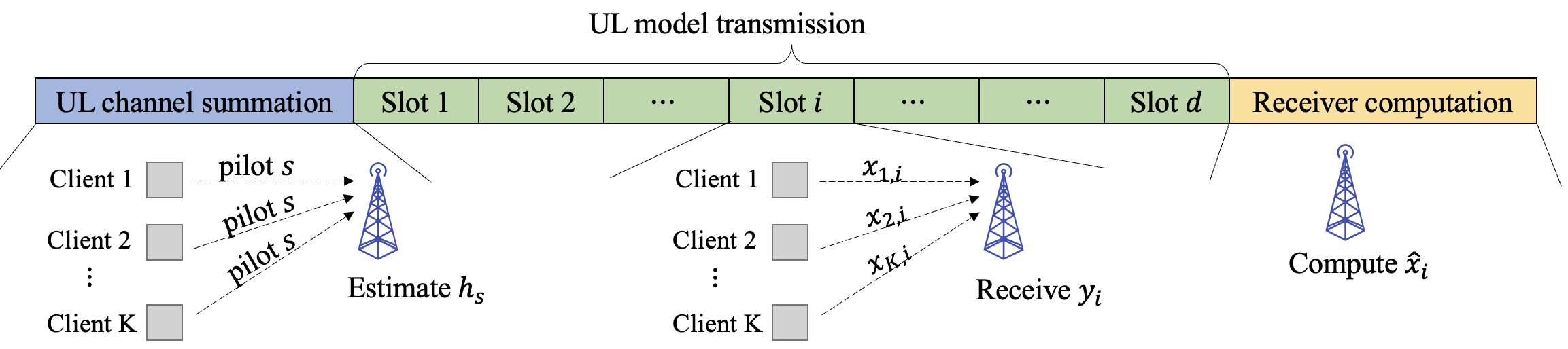
The designed framework contains the following three main steps in the uplink communications.

As shown in (a) of Eqn. (6), inner product ${\bf h}_{s}^{H}{\bf y}_{i}$ can be viewed as the combination of three parts: signal, interference, and noise. We next show that, taking advantage of two fundamental properties of massive MIMO, the error-free approximation (b) in (6) is asymptotically accurate (as the number of BS antennas $M$ goes to infinity).

To gain some insight of random orthogonality, we approximate the average signal-to-interference-plus-noise-ratio (SINR) after the operation in (6) as

which grows linearly with $M$ for a fixed $K$. On the other hand, for a given number of antennas $M$, Eqn. (9) can be used to guide the choice of $K$ in each communication round to satisfy an SINR requirement. We will provide more details on the scalability of clients via the convergence analysis of FL with random orthogonalization in Section VI-B. We note that Eqn. (9) is an approximate expression for SINR but it sheds light into the relationship between $K$ and $M$. This approximation, however, is not used in the convergence analysis of FL with random orthogonalization in Section VI-B.

Inspired by the uplink communication design, the downlink design contains the following two steps.

In the uplink communication, recall that the received signal is ${\bf y}_{i}={\bf H}{\bf x}_{i}+{\bf n}_{i}$. Denoting $\mbox{\boldmath$\mu$\unboldmath}_{\textrm{$\sf{UL}$}{}}={\bf H}{\bf x}_{i}$, we have ${\bf y}_{i}\sim\mathcal{CN}(\mbox{\boldmath$\mu$\unboldmath}_{\textrm{$\sf{UL}$}{}},\frac{1}{\textrm{$\sf{SNR}$}{}}{\bf I})$. To leverage CRLBs to evaluate the parameter estimation, we first need to derive the Fisher information of ${\bf x}_{i}$. Based on Example $3.9$ in [53], we can write the Fisher information matrix (FIM) of the estimation of ${\bf x}_{i}$ as:

After inserting $\frac{\partial\mbox{\boldmath$\mu$\unboldmath}_{\textrm{$\sf{UL}$}{}}({\bf x}_{i})}{\partial{\bf x}_{i}}={\bf H}$ into the FIM, we have ${\bf F}_{\textrm{$\sf{UL}$}{}}=2\cdot\textrm{$\sf{SNR}$}{}\cdot\real({\bf H}^{H}{\bf H})$. Note that for the enhanced uplink design, we can absorb $\real(g_{k})$ into the effective channel as $\tilde{\bf H}\triangleq\left[{\bf h}_{1}/\real(g_{1}),\cdots,{\bf h}_{K}/\real(g_{K})\right]$, and calculate FIM via ${\bf F}_{\textrm{$\sf{UL}$}{}}=2\cdot\textrm{$\sf{SNR}$}{}\cdot\real(\tilde{\bf H}^{H}\tilde{\bf H})$.

In the downlink communication, since $y_{k}={\bf h}_{k}^{H}{\bf h}_{s}w_{i}+{\bf n}_{k}$, by the definition of $\mu_{\textrm{$\sf{DL}$}{}}={\bf h}_{k}^{H}{\bf h}_{s}w_{i}$, we have that $y_{k}\sim\mathcal{CN}(\mu_{\textrm{$\sf{DL}$}{}},\frac{1}{\textrm{$\sf{SNR}$}{}})$. The Fisher information of global model parameters is

The CRLBs of estimates are then given by the inverse of the Fisher information (matrix): ${\bf C}_{\hat{\bf x}_{i}}={\bf F}_{\textrm{$\sf{UL}$}{}}^{-1}$ and $C_{\hat{w}_{i}}=1/F_{\textrm{$\sf{DL}$}{}}$, respectively. CRLBs are the lower bounds on the variances of unbiased estimators, stating that the variance of any such estimator is at least as high as the inverse of the Fisher information (matrix). We have shown that the proposed methods lead to unbiased estimations of the global model in both uplink and downlink communications. Hence, we can use the sum of all diagonal elements of ${\bf C}_{\hat{\bf x}}$ as the lower bound of the mean squared error (MSE) $\mathbb{E}\left\|{\bf x}_{i}-\hat{\bf x}_{i}\right\|^{2}$, and use $C_{\hat{w}_{i}}$ as the lower bound of MSE $\mathbb{E}\left\|w_{i}-\hat{w}_{i}\right\|^{2}$, to evaluate the performance of model estimation in both uplink and downlink communications. These bounds will be validated in the experiment results.

We now analyze the ML model convergence performances of the proposed methods. Note that as we have proposed two different designs (basic and enhanced) for the uplink and downlink communications, respectively, there would be four cases of convergence analysis. Since these convergence analyses are quite similar, we only report one of these results.

We first make the following standard assumptions that are commonly adopted in the convergence analysis of FedAvg and its variants [16, 54, 14, 55]. In particular, Assumption 1 indicates that the gradient of $f_{k}$ is Lipschitz continuous. The strongly convex loss function in Assumption 2 is a category of loss functions that are widely studied in the literature (see [16] and its follow-up works). Assumptions 3 and 4 imply that the mini-batch stochastic gradient and its variance are bounded [14].

We next provide a convergence analysis of FL when the uplink communication utilizes random orthogonalization and the enhanced design is applied to the downlink communication. Note that unlike uplink communications, we cannot use model differential for downlink FL communications because of partial clients selection. To guarantee the convergence of FL, we need to borrow the necessary condition for noisy FL downlink communication from our previous work [56], i.e., downlink transmit power should scale in the order of $\mathcal{O}(t^{2})$.

Theorem 1 shows that applying random orthogonalization in the uplink communications and enhanced method in the downlink communications preserves the $\mathcal{O}(1/T)$ convergence rate of vanilla SGD in FL tasks with perfect communications in both uplink and downlink phases. The factors that impact the convergence rate are captured entirely in the constant $B$, which come from multiple sources as explained below: $\frac{\sum_{k\in[N]}H_{k}^{2}}{N^{2}}$ comes from the variances of stochastic gradients; $6L\Gamma$ is introduced by the non-i.i.d. of local datasets; the choice of local computation steps and the fraction of partial client participation lead to $8(E-1)^{2}H^{2}$ and $\frac{N-K}{N-1}\frac{4}{K}E^{2}H^{2}$, respectively; and the interference and noise in uplink and downlink communications result in $\frac{4}{K}\left(\frac{K}{M}+\frac{1}{\textrm{$\sf{SNR}$}{}_{\textrm{$\sf{UL}$}{}}}\right)E^{2}H^{2}$ and $\left(d+\frac{dK}{M}\right)$, respectively. Note that the impact of the downlink noise, i.e., $\textrm{$\sf{SNR}$}{}_{\textrm{$\sf{DL}$}{}}$, is not explicit in $B$ due to the requirement of $\textrm{$\sf{SNR}$}{}_{\textrm{$\sf{DL}$}{}}\geq\frac{1-\mu\eta_{t}}{\eta^{2}_{t}}$ to guarantee the convergence.

We next analyze the relationship between the number of selected clients $K$ and the number of BS antennas $M$ to understand the scalability of multi-user MIMO for FL, which provides more insight for practical system design. To this end, we consider a simplified case where the system only configures random orthogonalization in the uplink communications, assuming that the downlink communications are error-free. Note that this configuration is reasonable when the BS has large transmit power. We further assume full client participation ($N=K$), one-step SGD at each device ($E=1$), and i.i.d datasets across all clients ($\Gamma=0$). For this special case, we establish Corollary 2 as follows.

Corollary 2 shows that there are two main factors that impact the convergence rate of FL with MIMO: variance reduction and channel interference and noise. In particular, the definition of $\tilde{B}$ in (18), which appears in Corollary 2, captures the joint impact of both factors. The nature of distributed SGD suggests that, for a fixed mini-batch size at each client, involving $K$ devices enjoys a $\frac{1}{K}$ variance reduction of stochastic gradient at each SGD iteration [58], which is captured by the $\frac{H^{2}}{K}$ term in (18). However, due to the existence of interference and noise, the convergence rate is determined by both factors, shown as $\frac{H^{2}}{K}$ and $\frac{(K/M+1/\textrm{$\sf{SNR}$}{})H^{2}}{K}\approx\frac{H^{2}}{M}$ terms in (18). This suggests that the desired variance reduction may be adversely impacted if channel interference and noise dominate the convergence bound. In particular, when $M\gg K$, we have $\frac{1}{K}\gg\frac{1}{M}$, and the system enjoys almost the same variance reduction as the interference-free and noise-free case. However, in the case of $K\gg M$, we have $\frac{(K/M+1/\textrm{$\sf{SNR}$}{})}{K}\approx\frac{1}{M}\gg\frac{1}{K}$, and $\frac{H^{2}}{M}$ dominates the convergence bound. In this case, it is unwise to blindly increase the number of clients, as it does not have the advantage of variance reduction.

We consider a massive MIMO BS with $M=256$, $512$, or $1024$ antennas, with $K=8$ active users participating in an FL task. We assume a Rayleigh fading channel model, i.e., ${\bf h}_{k}\sim\mathcal{CN}(0,\frac{1}{M}{\bf I})$, for each user, and use the MSE of the computed global model parameters in uplink and downlink communications to evaluate the system performance. All MSE results are obtained from $2000$ Monte Carlo experiments. We use CRLBs derived in Section VI-A as the benchmarks of the computed MSEs. In addition, we adopt the traditional MIMO MMSE estimator and the semidefinite relaxation based (SDR-based) precoder design method in [50] for performance comparisons of uplink and downlink communications, respectively.

Similarly, Fig. 5(c) and Fig. 5(d) compare the MSE performance of the enhanced method in uplink and downlink communications with the MMSE estimator / SDR-based precoder. It is clear from both plots that the enhanced method achieves MSEs very closed to the CRLBs. Furthermore, it performs nearly identically as the MMSE estimator in uplink and outperforms the SDR-based method by about $1.5$ dB in downlink. Therefore, by introducing channel echos, the enhanced method achieves excellent performance while consuming relatively low additional resource.

We next evaluate the performance when the estimation of the summation channel ${\bf h}_{s}$ (and $g_{k}$ in the enhanced method) is imperfect. The right sub-figure of Fig. 6 compares the MSEs of both proposed methods when the channel estimation is obtained under $\textrm{$\sf{SNR}$}{}=20$ dB. It reveals that the downlink communication is more robust than the uplink – the former achieves nearly identical MSEs as the ideal case even when the channel estimation is inaccurate. For the uplink, an imperfect channel estimation increases the MSEs by $1\sim 3$ dB depending on the antenna configurations. However, we emphasize again that the FL tasks have the same convergence rate under a constant SINR in the uplink communications (thanks to the model differential transmission).

To evaluate the ML performance, we carry out experiments of FL classification tasks using two widely adopted real-world datasets: MNIST and CIFAR-10, via a support vector machine (SVM) model and a convolution neural network (CNN) model, respectively.

Fig. 7(a) and Fig. 7(b) report the training loss and test accuracy when the uplink adopts the proposed method, and the downlink is assumed to be noise-free. The uplink SNR is set as $10$ dB. We can see that both random orthogonalization and the enhanced method behave almost identically as the ideal case where both uplink and downlink communications are perfect. Note that although the global model received at the BS has noise and interference components, the actual learning performances of the two methods do not deteriorate. Due to the model differential transmission in the uplink communications, the effective SINR of the received global model gradually increases as the model converges, despite the presence of channel interference and noise. Fig. 7(c) and Fig. 7(d) demonstrate the learning performance when the proposed designs are applied to the downlink communications. Since the model differential transmission is infeasible, we set the initial downlink SNR as $0$ dB and scale at a rate of $\mathcal{O}(t^{2})$ as the learning progresses (see [56]). We notice that the learning performance of the enhanced method is almost identical to that of the ideal case, while there exists a performance gap of about $2\%$ test accuracy loss of random orthogonalization.

Fig. 7(e) and Fig. 7(f) illustrate the training loss and test accuracy versus the learning rounds when both the uplink and downlink communications adopt the random orthogonalization method or the enhanced method, respectively. It is observed that the enhanced method achieves similar training loss and test accuracy as the ideal case. Due to the constant interference in the downlink communications, random orthogonalization incurs a test accuracy loss of about $3\%$.

To summarize, experiments on both datasets demonstrate that random orthogonalization suffers a slight performance degradation over the ideal case when it is applied to the downlink communications. As we have stated in Remark 5, unlike the enhanced method that cancels all interference in the received global model, the interference is constant in the global model obtained via random orthogonalization despite the increased SNR. Note that this gap can be reduced by increasing $M$. Therefore, downlink random orthogonalization is more attractive in systems with large number of antennas or severely limited resources.

References

- [1] X. Wei, C. Shen, J. Yang, and H. V. Poor, “Random orthogonalization for federated learning in massive MIMO systems,” in Proc. IEEE International Conference on Communications (ICC), May 2022, pp. 1–6.
- [2] B. McMahan, E. Moore, D. Ramage, S. Hampson, and B. A. y Arcas, “Communication-efficient learning of deep networks from decentralized data,” in Proc. AISTATS, Fort Lauderdale, FL, USA, Apr. 2017, pp. 1273–1282.
- [3] J. Konecny, H. B. McMahan, F. X. Yu, P. Richtarik, A. T. Suresh, and D. Bacon, “Federated learning: Strategies for improving communication efficiency,” in Proc. NIPS Workshop on Private Multi-Party Machine Learning, 2016.
- [4] M. Chen, N. Shlezinger, H. V. Poor, Y. C. Eldar, and S. Cui, “Communication-efficient federated learning,” Proceedings of the National Academy of Sciences, vol. 118, no. 17, p. e2024789118, 2021.
- [5] S. Niknam, H. S. Dhillon, and J. H. Reed, “Federated learning for wireless communications: Motivation, opportunities, and challenges,” IEEE Commun. Mag., vol. 58, no. 6, pp. 46–51, 2020.
- [6] G. Zhu, Y. Wang, and K. Huang, “Broadband analog aggregation for low-latency federated edge learning,” IEEE Trans. Wireless Commun., vol. 19, no. 1, pp. 491–506, 2020.
- [7] X. Cao, G. Zhu, J. Xu, and K. Huang, “Optimized power control for over-the-air computation in fading channels,” IEEE Trans. Wireless Commun., vol. 19, no. 11, pp. 7498–7513, 2020.
- [8] D. Tse and P. Viswanath, Fundamentals of Wireless Communication. Cambridge University Press, 2005.
- [9] A. Goldsmith, Wireless Communications. Cambridge University Press, 2005.
- [10] K. Yang, T. Jiang, Y. Shi, and Z. Ding, “Federated learning via over-the-air computation,” IEEE Trans. Wireless Commun., vol. 19, no. 3, pp. 2022–2035, 2020.
- [11] A. M. Elbir and S. Coleri, “Federated learning for hybrid beamforming in mm-Wave massive MIMO,” IEEE Commun. Letter, vol. 24, no. 12, pp. 2795–2799, 2020.
- [12] T. Huang, B. Ye, Z. Qu, B. Tang, L. Xie, and S. Lu, “Physical-layer arithmetic for federated learning in uplink MU-MIMO enabled wireless networks,” in Proc. IEEE Conference on Computer Communications (INFOCOM), 2020, pp. 1221–1230.
- [13] Y.-S. Jeon, M. M. Amiri, J. Li, and H. V. Poor, “A compressive sensing approach for federated learning over massive MIMO communication systems,” IEEE Trans. Wireless Commun., vol. 20, no. 3, pp. 1990–2004, 2020.
- [14] S. U. Stich, “Local SGD converges fast and communicates little,” in Proc. International Conference on Learning Representations (ICLR), 2018.
- [15] J. Wang and G. Joshi, “Cooperative SGD: A unified framework for the design and analysis of communication-efficient SGD algorithms,” in Proc. ICML Workshop on Coding Theory for Machine Learning, 2019.
- [16] X. Li, K. Huang, W. Yang, S. Wang, and Z. Zhang, “On the convergence of FedAvg on non-IID data,” in Proc. International Conference on Learning Representations (ICLR), 2020.
- [17] K. Thonglek, K. Takahashi, K. Ichikawa, C. Nakasan, P. Leelaprute, and H. Iida, “Sparse communication for federated learning,” in Proc. IEEE 6th International Conference on Fog and Edge Computing (ICFEC), 2022, pp. 1–8.
- [18] Y. Oh, Y.-S. Jeon, M. Chen, and W. Saad, “FedVQCS: Federated learning via vector quantized compressed sensing,” arXiv preprint arXiv:2204.07692, 2022.
- [19] G. Zhu, Y. Du, D. Gündüz, and K. Huang, “One-bit over-the-air aggregation for communication-efficient federated edge learning: Design and convergence analysis,” IEEE Trans. Wireless Commun., vol. 20, no. 3, pp. 2120–2135, 2021.
- [20] M. M. Amiri, D. Gunduz, S. R. Kulkarni, and H. V. Poor, “Federated learning with quantized global model updates,” arXiv preprint arXiv:2006.10672, 2020.
- [21] Y. Du, S. Yang, and K. Huang, “High-dimensional stochastic gradient quantization for communication-efficient edge learning,” IEEE Trans. Signal Processing, vol. 68, pp. 2128–2142, 2020.
- [22] D. Wen, K.-J. Jeon, M. Bennis, and K. Huang, “Adaptive subcarrier, parameter, and power allocation for partitioned edge learning over broadband channels,” IEEE Trans. Wireless Commun., vol. 20, no. 12, pp. 8348–8361, 2021.
- [23] H. Chen, S. Huang, D. Zhang, M. Xiao, M. Skoglund, and H. V. Poor, “Federated learning over wireless IoT networks with optimized communication and resources,” IEEE Internet Things J., vol. 9, no. 17, pp. 16 592–16 605, 2022.
- [24] S. Wang, M. Chen, C. Yin, W. Saad, C. S. Hong, S. Cui, and H. V. Poor, “Federated learning for task and resource allocation in wireless high-altitude balloon networks,” IEEE Internet Things J., vol. 8, no. 24, pp. 17 460–17 475, 2021.
- [25] B. Nazer and M. Gastpar, “Computation over multiple-access channels,” IEEE Trans. Info. Theory, vol. 53, no. 10, pp. 3498–3516, 2007.
- [26] M. M. Amiri and D. Gündüz, “Federated learning over wireless fading channels,” IEEE Trans. Wireless Commun., vol. 19, no. 5, pp. 3546–3557, 2020.
- [27] M. Chen, H. V. Poor, W. Saad, and S. Cui, “Convergence time optimization for federated learning over wireless networks,” IEEE Trans. Wireless Commun., vol. 20, no. 4, pp. 2457–2471, 2020.
- [28] J. Xu and H. Wang, “Client selection and bandwidth allocation in wireless federated learning networks: A long-term perspective,” IEEE Trans. Wireless Commun., vol. 20, no. 2, pp. 1188–1200, 2021.
- [29] Y. Sun, S. Zhou, Z. Niu, and D. Gündüz, “Dynamic scheduling for over-the-air federated edge learning with energy constraints,” IEEE J. Select. Areas Commun., vol. 40, no. 1, pp. 227–242, 2021.
- [30] X. Ma, H. Sun, Q. Wang, and R. Q. Hu, “User scheduling for federated learning through over-the-air computation,” in Proc. IEEE 94th Vehicular Technology Conference (VTC2021-Fall), 2021, pp. 1–5.
- [31] H.-S. Lee and J.-W. Lee, “Adaptive transmission scheduling in wireless networks for asynchronous federated learning,” IEEE J. Select. Areas Commun., vol. 39, no. 12, pp. 3673–3687, 2021.
- [32] M. M. Wadu, S. Samarakoon, and M. Bennis, “Joint client scheduling and resource allocation under channel uncertainty in federated learning,” IEEE Trans. Commun., vol. 69, no. 9, pp. 5962–5974, 2021.
- [33] T. Sery and K. Cohen, “On analog gradient descent learning over multiple access fading channels,” IEEE Trans. Signal Processing, vol. 68, pp. 2897–2911, 2020.
- [34] Z. Lin, X. Li, V. K. Lau, Y. Gong, and K. Huang, “Deploying federated learning in large-scale cellular networks: Spatial convergence analysis,” IEEE Trans. Wireless Commun., vol. 21, no. 3, pp. 1542–1556, 2021.
- [35] O. Aygün, M. Kazemi, D. Gündüz, and T. M. Duman, “Over-the-air federated learning with energy harvesting devices,” arXiv preprint arXiv:2205.12869, 2022.
- [36] S. Wan, J. Lu, P. Fan, Y. Shao, C. Peng, and K. B. Letaief, “Convergence analysis and system design for federated learning over wireless networks,” IEEE J. Select. Areas Commun., vol. 39, no. 12, pp. 3622–3639, 2021.
- [37] T. Sery, N. Shlezinger, K. Cohen, and Y. C. Eldar, “Over-the-air federated learning from heterogeneous data,” IEEE Trans. Signal Processing, vol. 69, pp. 3796–3811, 2021.
- [38] Y. Sun, S. Zhou, Z. Niu, and D. Gündüz, “Time-correlated sparsification for efficient over-the-air model aggregation in wireless federated learning,” in Proc. IEEE International Conference on Communications (ICC), May 2022, pp. 1–6.
- [39] T. T. Vu, H. Q. Ngo, M. N. Dao, D. T. Ngo, E. G. Larsson, and T. Le-Ngoc, “Energy-efficient massive MIMO for federated learning: Transmission designs and resource allocations,” arXiv preprint arXiv:2112.11723, 2021.
- [40] R. Hamdi, M. Chen, A. B. Said, M. Qaraqe, and H. V. Poor, “Federated learning over energy harvesting wireless networks,” IEEE Internet Things J., vol. 9, no. 1, pp. 92–103, 2021.
- [41] T. T. Vu, D. T. Ngo, H. Q. Ngo, M. N. Dao, N. H. Tran, and R. H. Middleton, “Joint resource allocation to minimize execution time of federated learning in cell-free massive MIMO,” IEEE Internet Things J., vol. Early access, 2022.
- [42] T. T. Vu, D. T. Ngo, N. H. Tran, H. Q. Ngo, M. N. Dao, and R. H. Middleton, “Cell-free massive MIMO for wireless federated learning,” IEEE Trans. Wireless Commun., vol. 19, no. 10, pp. 6377–6392, 2020.
- [43] Y. Mu, N. Garg, and T. Ratnarajah, “Communication-efficient federated learning for massive MIMO systems,” in Proc. IEEE Wireless Communications and Networking Conference (WCNC), 2022, pp. 578–583.
- [44] C. Xu, S. Liu, Z. Yang, Y. Huang, and K.-K. Wong, “Learning rate optimization for federated learning exploiting over-the-air computation,” IEEE J. Select. Areas Commun., vol. 39, no. 12, pp. 3742–3756, 2021.
- [45] Z. Lin, Y. Gong, and K. Huang, “Distributed over-the-air computing for fast distributed optimization: Beamforming design and convergence analysis,” arXiv preprint arXiv:2204.06876, 2022.
- [46] C. Zhong, H. Yang, and X. Yuan, “Over-the-air federated multi-task learning over MIMO multiple access channels,” arXiv preprint arXiv:2112.13603, 2021.
- [47] S. Xia, J. Zhu, Y. Yang, Y. Zhou, Y. Shi, and W. Chen, “Fast convergence algorithm for analog federated learning,” in Proc. IEEE International Conference on Communications (ICC), June 2021, pp. 1–6.
- [48] M. M. Amiri, T. M. Duman, D. Gündüz, S. R. Kulkarni, and H. V. Poor, “Blind federated edge learning,” IEEE Trans. Wireless Commun., vol. 20, no. 8, pp. 5129–5143, 2021.
- [49] B. Tegin and T. M. Duman, “Blind federated learning at the wireless edge with low-resolution adc and dac,” IEEE Transactions on Wireless Communications, vol. 20, no. 12, pp. 7786–7798, 2021.
- [50] N. Sidiropoulos and T. Davidson, “Broadcasting with channel state information,” in Proc. of 2004 Sensor Array and Multichannel Signal, 2004, pp. 489–493.
- [51] S. Sesia, I. Toufik, and M. Baker, LTE - The UMTS Long Term Evolution: From Theory to Practice, 2nd ed. Wiley, 2011.
- [52] H. Q. Ngo, E. G. Larsson, and T. L. Marzetta, “Aspects of favorable propagation in massive MIMO,” in Proc. IEEE 22nd European Signal Processing Conference (EUSIPCO), 2014, pp. 76–80.
- [53] S. M. Kay, Fundamentals of statistical signal processing: estimation theory. Prentice-Hall, Inc., 1993.
- [54] P. Jiang and G. Agrawal, “A linear speedup analysis of distributed deep learning with sparse and quantized communication,” in Advances in Neural Information Processing Systems, 2018, pp. 2525–2536.
- [55] S. Zheng, C. Shen, and X. Chen, “Design and analysis of uplink and downlink communications for federated learning,” IEEE J. Select. Areas Commun., vol. 39, no. 7, pp. 2150–2167, July 2021.
- [56] X. Wei and C. Shen, “Federated learning over noisy channels: Convergence analysis and design examples,” IEEE Trans. Cogn. Commun. Netw., vol. 8, no. 2, pp. 1253–1268, 2022.
- [57] X. Wei, C. Shen, J. Yang, and H. V. Poor, “Technical report: Random orthogonalization for federated learning in massive MIMO systems,” http://www.ece.virginia.edu/~cs7dt/tech.pdf, University of Virginia, Tech. Rep., Aug. 2022.
- [58] R. Johnson and T. Zhang, “Accelerating stochastic gradient descent using predictive variance reduction,” Advances in Neural Information Processing Systems, vol. 26, pp. 315–323, 2013.
- [59] L. Deng, “The MNIST database of handwritten digit images for machine learning research,” IEEE Signal Process. Mag., vol. 29, no. 6, pp. 141–142, 2012.
- [60] H. Mania, X. Pan, D. Papailiopoulos, B. Recht, K. Ramchandran, and M. I. Jordan, “Perturbed iterate analysis for asynchronous stochastic optimization,” SIAM Journal on Optimization, vol. 27, no. 4, pp. 2202–2229, 2017.