11CCS: Security and privacy Security services

Xiaoyu Fan email: fanxy20@mails.tsinghua.edu.cn Affiliation: IIIS, Tsinghua University , Kun Chen email: chenkun@tsingj.com Affiliation: Tsingjiao Information Technology Co. Ltd. , Guosai Wang email: guosai.wang@tsingj.com Affiliation: Tsingjiao Information Technology Co. Ltd. , Mingchun Zhuang email: mczhuang@bupt.edu.cn Affiliation: Beijing University of Posts and Telecommunications , Yi Li email: xiaolixiaoyi@tsingj.com Affiliation: Tsingjiao Information Technology Co. Ltd. and Wei Xu email: weixu@tsinghua.edu.cn Affiliation: IIIS, Tsinghua University

2022; © acmcopyright

Abstract.

Due to the absence of a library for non-linear function evaluation, so-called general-purpose secure multi-party computation (MPC) are not as “general” as MPC programmers expect. Prior arts either naively reuse plaintext methods, resulting in suboptimal performance and even incorrect results, or handcraft ad hoc approximations for specific functions or platforms. We propose a general technique, NFGen ¹¹ 1 The source code is released in https://github.com/Fannxy/NFGen, that utilizes pre-computed discrete piecewise polynomials to accurately approximate generic functions using fixed-point numbers. We implement it using a performance-prediction-based code generator to support different platforms. Conducting extensive evaluations of 23 non-linear functions against six MPC protocols on two platforms, we demonstrate significant performance, accuracy, and generality improvements over existing methods.

Keywords:

Secure Multi-Party Computation (MPC), Non-linear Function Evaluation, Automatic Code Generation

1. Introduction

Privacy-preserving computation, especially secure multi-party computation (MPC), has attracted a lot of attention in both academia and industry. They provide a promising trade-off between mining the data and privacy protection. People have proposed many general-purpose MPC platforms (Keller 2020; Li and Xu 2019; Mohassel and Zhang 2017; Knott et al. 2021; Bogdanov et al. 2008; Tan et al. 2021) that provide high-level abstractions and practical performance, allowing people to develop secure data processing applications without understanding the details of underlying MPC protocols.

Most platforms use a version of secret sharing (SS) protocols to build basic secure operations like $\mathsf{+}$ , $\mathsf{\times}$ , and comparison (e.g., $\mathsf{>}$ ), and then construct complex functions by composing them, just like writing plaintext expressions. The security of compound operations/functions is guaranteed by the universal composability (Canetti 2001) of these protocols. These platforms usually provide built-in support for common non-linear functions such as reciprocal ( $\frac{1}{x}$ , for real number divisions), exponential ( $e^{x}$ ), logarithm ( $\ln{x}$ ), and square root ( $\sqrt{x}$ ). They implement these functions either using generic numerical methods (e.g. the Newton method) or adopting protocol-specific algorithms like in (Rathee et al. 2021; Damgård et al. 2019).

It remains a big challenge, however, to support the large variety non-linear functions in scientific computing and machine learning, such as $\chi^{2}test$ and sigmoid. The naive approach is to compose them with built-in functions. E.g., we can compute $tanh(x)=\frac{e^{x}-e^{-x}}{e^{x}+e^{-x}}$ by composing two $e^{x}$ , one $\frac{1}{x}$ and two $\mathsf{+}$ . We refer to this approach as direct evaluation. Unfortunately, there are four pitfalls.

Pitfall 1: Correctness and precision. Most practical MPC platforms use fixed-point (FXP) numbers instead of the common floating-point (FLP) ones for efficiency. Although there are attempts to support FLP in MPC (Aliasgari et al. 2013), the low performance for $\mathsf{+}$ prevents people from adopting it. FXP still dominates the practical MPC platforms (Keller 2020; Li and Xu 2019; Mohassel and Zhang 2017; Knott et al. 2021; Tan et al. 2021; Bogdanov et al. 2008). Unfortunately, ignoring the differences between FXP and FLP leads to two severe issues:

First, FXP supports a much smaller range and resolution than FLP, leading to more overflow/underflow as well as precision loss. Even worse, FXP cannot represent $NaN$ and $Inf$ like FLP. Also, the inputs/outputs on MPC are in ciphertext, so there is no way to detect overflows. Using $tanh$ as an example, even if the function has a range of $[-1,1]$ , the intermediate results, $e^{x}$ and $e^{-x}$ , can easily overflow when $|x|$ is large. In plaintext, people use a scaling conversion to enlarge the range of FXP, but in MPC, the encrypted $x$ makes scaling costly. In fact, the built-in $tanh$ function in MP-SPDZ (Keller 2020) gives wrong results if $|x|>44$ , even if we increase FXP width to 128 bits. Second, each non-linear function has a precision loss that accumulates if we compose them with multiple steps. Section 7.3 shows more examples of both issues.

Pitfall 2: Performance. Even with aggressive optimizations, non-linear function evaluation takes significant time using MPC. Depending on the platform, they can be orders of magnitude slower than the plaintext version. We measure the relative performance between non-linear functions vs. basic operations in 6 MPC protocols and observe dramatic differences (Table 1 in Section 7.1). Composing these functions sequentially makes things even slower.

Pitfall 3: Generality. Although we can write many non-linear functions using the built-ins, some functions are hard to implement. For example, functions $\gamma(x,z)$ , $\Gamma{(x,z)}$ and $\Phi{(x)}$ are defined as integrals. It is very tedious, if not impossible, to implement them in MPC using numerical methods and built-in operations.

Pitfall 4: Portability. Even if we can afford the engineering effort to build a complete scientific computation library, there are too many performance trade-offs to make it portable to different MPC systems and applications. MPC systems use a variety of protocols (to support different security assumptions), number representations and sizes, as well as custom programming languages. Also, they are deployed in different hardware/software/network environments. We want the computation library to maintain efficiency in all cases with minimal porting efforts.

In this paper, we offer a new scheme, non-linear function code generator (NFGen), to evaluate non-linear functions on general-
purpose MPC platforms. We approximate each non-linear function using an $m$ -piece piecewise polynomial with max order $k$ (we automatically determine $k$ and $m$ ). Our approach has three advantages. First, it only uses secure $\mathsf{+}$ , $\mathsf{\times}$ and $\mathsf{>}$ operations supported by all popular MPC platforms, and we can prove that the security properties are the same as the underlying platform with the same adversarial models. Second, the evaluation is oblivious, i.e., the operation sequence is not dependent on input data, allowing for predictable running time and avoiding timing-related side-channels. Third, obtaining the approximation is independent of input data and hence can be precomputed on plaintext.

Key challenges. Finding a good $(k,m)$ -piecewise polynomial approximation for MPC platforms is a challenging problem. First, fitting polynomials for FXP computation introduces many challenges: 1) the polynomial needs to meet both the range and the resolution requirements of FXP, making sure all intermediate steps neither overflow nor underflow; 2) an FXP is essentially an integer, making the polynomials discrete. Fitting one polynomial minimizing the approximation error is an NP-complete integer programming (IP) problem. Thus we need to find an approximation. Second, there is a trade-off between $m$ and $k$ : whether we get more pieces (mainly leading to more $\mathsf{>}$ ’s) or use a higher-order polynomial (leading to more $\mathsf{\times}$ ’s). The choice depends on the performance of the specific MPC system, as we discussed above.

Method overview. We compute the polynomial fitting as a pre-computation step in plaintext. In a nutshell, we first construct a polynomial with order $k$ in FLP using Chebyshev Interpolation (Trefethen 2019) (or Lagrange Interpolation (MathWorld 2015) for corner case) and then discretized it into FXP. We check the accuracy of the FXP polynomial using random data samples. If it does not achieve the user-specified accuracy, we split the input domain into two and recurse on each smaller domain. We design a series of algorithms leveraging the FLP capability to help find a better FXP approximation, like using two FXPs to expand the range and improving the precision through residual functions. Section 4 provides the details of the algorithms.

At runtime, we evaluate the $(k,m)$ -piecewise polynomial in an oblivious way, i.e. the execution only depends on $(k,m)$ , but not input data. We design an oblivious piecewise polynomial evaluation (OPPE) algorithm (Section 4.3). To get a good $(k,m)$ trade-off on different MPC platforms, NFGen uses a profiler to collect performance metrics of a specific deployment of an MPC platform and learns a model to predict the performance with different $(k,m)$ . NFGen automatically makes the choice using the prediction and generates MPC-platform-specific OPPE code using built-in code templates. NFGen provides templates for both PrivPy (Li and Xu 2019) and MP-SPDZ (Keller 2020). The template is the only platform-dependent part in NFGen, and it only takes a short template to port NFGen to a new MPC platform.

Evaluation results. We evaluate NFGen against 6 secret sharing protocols using $15$ commonly used non-linear functions on both PrivPy (Li and Xu 2019) and MP-SPDZ (Keller 2020). We observe significant performance improvements over baselines (direct evaluation) in $93\%$ of all cases with an average speedup of $6.5\times$ and a maximum speedup of $86.1\times$ . NFGen saves $39.3\%$ network communications on average. We also show that we can avoid the overflow errors and achieve much better accuracy comparing with the baseline, and allow a larger input domain even with small FXP widths. Using logistic regression (LR) as an example, we demonstrate performance and accuracy improvements over direct evaluation and ad hoc approximations, with $3.5\times$ speedup and $0.6\%-14\%$ accuracy improvements. Additionally, we illustrate how NFGen helps users to easily implement otherwise hard-to-implement functions on MPC by using 8 complex functions defined as integrals and the $\chi^{2}$ test on real data.

In summary, our contributions include:

1) We propose a series of algorithms to fit an effective piecewise polynomial approximation on plaintext, fully considering the differences between FLP and FXP representations.

2) We design and implement the code generator with automatic profiling to allow portability to different MPC systems with distinct performance characteristics.

3) We conduct comprehensive evaluations against six MPC protocols on two platforms over 23 non-linear functions, showing significant improvements in performance, accuracy, portability to different MPC platforms, usability and savings in communications.

Refer to caption — Figure 1. End-to-end Workflow of NFGen

2. Background and Related work

In this section, we first introduce the background of general-purpose MPC platforms and FXP numbers for readers unfamiliar with this area and then review related works.

2.1. General-purpose MPC Platforms

General-purpose MPC platforms usually provide a high-level programming front-end with a compiler/interpreter to translate a high-level code into a series of cryptographic building blocks (Hastings et al. 2019). They provide common operators like $\mathsf{+}$ , $\mathsf{\times}$ , $\mathsf{>}$ and $\frac{1}{x}$ in the front-end, and implement these operations using MPC protocols. These platforms guarantee privacy in the end-to-end algorithms based on the universal composability of the underlying security protocols. Example platforms include MP-SPDZ (Keller 2020), PrivPy (Li and Xu 2019), CrypTen (Knott et al. 2021), SecureML (Mohassel and Zhang 2017), ABY (Demmler et al. 2015), and CryptGPU (Tan et al. 2021) etc. They hugely lower the barriers of developing privacy-preserving applications.

Most of the general-purpose MPC platforms use secret sharing (SS) (Demmler et al. 2015; Li and Xu 2019; Knott et al. 2021; Mohassel and Zhang 2017; Tan et al. 2021) as the underlying protocol. There are a range of security assumptions (e.g., semi-honest vs. malicious) in these protocols, resulting in significantly differing performance. Some platforms allow users to choose the underlying protocols, like (Keller 2020). Our goal is to make NFGen protocol-agnostic.

Secret sharing protocols require communications among the participants on each operation, which results in significantly slower performance than plaintext (usually $10\times-1000\times$ slower, depending on the protocol and network environment). Also, different operators in the same protocol exhibit vast performance difference. For example, in the most common additive secret sharing protocol, $\mathsf{+}$ is almost as fast as plaintext as it is communication-free. However, $\mathsf{\times}$ and $\mathsf{>}$ require communication and are slower. Non-linear operations like $\frac{1}{x}$ and $\sqrt{x}$ operate more slowly. It is important to make $\mathsf{+}$ fast as it is the most common operation in many applications.

To make $\mathsf{+}$ fast, MPC systems need to avoid floating point (FLP) numbers because the ciphertext exponent in FLP prevents us from adding up FLPs directly. Thus, almost all practical MPC platforms use fixed-point (FXP) numbers (Mohassel and Zhang 2017; Tan et al. 2021; Knott et al. 2021; Mohassel and Rindal 2018; Li and Xu 2019; Catrina and Saxena 2010). FXP represents each real number as an $n$ -bit integer, out of which $f$ least significant bits represent the fraction, and the most significant bit is the sign. We denote it as a $\langle n,f\rangle$ -FXP number. In the $\langle n,f\rangle$ format, both the range and resolution of the FXP are fixed to $2^{n-f-1}$ and $2^{-f}$ , respectively. FXP offers a much smaller range and resolution than FLP, and thus programmers need to be more careful with overflows and precision losses. MPC further complicates the problem as we cannot detect overflows on ciphertext. Also, the common scaling method in plaintext FXP requires additional bit operations in ciphertext and thus becomes expensive in MPC.

2.2. Non-linear Functions in MPC Platforms

Lacking of a complete general numeric computation library, MPC application developers need to roll their application-specific solutions even for common functions, like logistic regression (LR) (Han et al. 2020), decision trees (Lindell and Pinkas 2000; Damgård et al. 2019), principal component analysis (PCA) (Fan et al. 2021) and neural networks (NNs) (Rathee et al. 2021; Tan et al. 2021; Knott et al. 2021). Mohassel et al. (Mohassel and Zhang 2017; Mohassel and Rindal 2018) use a 3-piece linear function to replace the slow sigmoid function in LR and NNs. However, there is no guarantee that the approximation maintains accuracy in all cases. In fact, we find cases with significant LR accuracy loss using this approximation.

The most straightforward method to evaluate non-linear functions in MPC is directly adapting the plaintext code and replacing basic operations to secure ones (e.g., $\mathsf{+}$ , $\mathsf{\times}$ and $\mathsf{>}$ ). For example, CrypTen (Knott et al. 2021) and CryptGPU (Tan et al. 2021) adopt a series of plaintext algorithms like Newton-Raphson iterations, limit approximations to implement $\frac{1}{x}$ , $e^{x}$ , $\sqrt{x}$ and $\ln{x}$ . Natively adopting plaintext code usually leads to poor performance, as we do not know when we have reached the desirable accuracy and need to iterate more.

There are also protocol-specific approaches. For example, Rathee et al. (Rathee et al. 2021) implement $10$ efficient cryptographic building blocks to support high-performance non-linear functions like reciprocal-of-sqrt, sigmoid and exponent. However, these functions are optimized for their 2-party-computation platform only. Similiarly, Damgård et al. (Damgård et al. 2019) propose a series of primitives to support efficient machine learning applications for SPD $\mathbb{Z}_{2^{k}}$ protocol (Cramer et al. 2018). More generally, Catrina et al. (Catrina and Saxena 2010) design a collection of general building-blocks suitable for any fixed-point MPC platform and propose an optimized $\frac{1}{x}$ primitive using Goldschmidt algorithm on secret FXP. MP-SPDZ (Keller 2020) uses the same algorithm.

Another line of methods is to approximate non-linear functions with polynomials. It is a well-studied problem in plaintext of finding an optimal polynomial approximating a given function $F(x)$ , minimizing the maximum difference over a given input domain $[a,b]$ . Such polynomial is referred to as minimax polynomial (Atkinson and Han 2005). Chebyshev interpolation (Trefethen 2019) is a well-known solution. It offers a close approximation to the minimax polynomial (so-called Chebyshev (near) minimax polynomial) (Atkinson and Han 2005; Trefethen 2019). Hesamifard et al. (Hesamifard et al. 2018) adopt the Chebyshev polynomial to evaluate sigmoid on homomorphic encryption. However, the range of FXP limits the order $k$ of the polynomial and prevents it from reaching the desired approximation accuracy either. Another challenge is that the limited resolution of FXP cannot capture sometimes-tiny coefficients in these polynomials. Previous work ignores this problem and leads to large errors (Hesamifard et al. 2018). Boura et al. (Boura 2018) propose to use Fourier series to approximate sigmoid in MPC platform. They work around the range and resolution issues using secure quadruple-precision FLP but brings in expensive computation overhead.

Unlike previous efforts, we adopt piecewise polynomial and fit a Chebyshev polynomial for each piece, resulting in improved accuracy. We take into account the differences between FXP and FLP and handle corner cases. Also, prior works focus on one or a few functions on a single MPC platform, whereas our goal is to build a general, cross-platform solution for all Lipschitz-continuous functions²² 2 Even if the functions are Lipschitz continuous, there is no theoretical guarantee that we will find a feasible approximation for all functions on any accuracy requirements. However, empirically, NFGen works well on all the functions we tested..

3. Overview

Notations and assumptions. We first describe the notations and assumptions we use throughout the paper. We assume $F(x)$ is a Lipschitz continuous function, and we can evaluate $F(x)$ in plaintext using FLP. NFGen approximates $F(x)$ by finding a set of feasible piecewise polynomials with different max order $k$ and the number of pieces $m$ . We denote the set of all feasible polynomials as $\mathcal{\hat{P}}$ $=\{\text{{$\hat{p}_{k}^{m}$} }\}$ . Each of the $\hat{p}_{k}^{m}$ contains $m$ pieces covering the entire input domain of $[a,b]$ as $[w_{0},w_{1},\dots,w_{j},\dots,w_{m}]$ ( $w_{0}=a$ and $w_{m}=b$ ). In each piece $j,(i.e.,[w_{j-1},w_{j}])$ , we have a polynomial $\hat{p}^{(j)}_{k}({\hat{x}})=\sum_{i=0}^{k}{{\hat{c}}_{i}{\hat{x}}^{i}}$ to approximate it. When the piece index $j$ is not important, we use a shorthand of $\hat{p}_{k}$ $(x)$ to denote it. Throughout the paper, symbols with a hat ( ${\hat{\cdot}}$ ) denote $\langle n,f\rangle$ -FXP representable variables and the definition of functions like $\hat{p}_{k}^{m}$ means all the coefficients and terms are in $\langle n,f\rangle$ -FXP representation (Section 2.1). We assume 64-bit double-precision FLP is equivalent to $\mathbb{R}$ . It is a safe assumption in our situation, considering both the resolution and range of FLP are orders of magnitudes larger than FXP of our concern.

NFGen input files. NFGen generates non-linear function approximation code for different MPC platforms according to two input files. The first is a user-provided non-linear function definition (NFD), containing the expression of the target function $F(x)$ , its domain $[a,b]$ , FXP format $\langle n,f\rangle$ , target accuracy $\epsilon$ and ${\hat{0}}$ (in Eq. 1), and a list of the operators supported by the target MPC platform. The users can generate the second input file, performance profile definition (PPD), running a NFGen-provided profiler on the target MPC platform deployment. Note that NFD is MPC-platform-specific but independent of the actual deployment (i.e., the CPU and networking configurations), and PPD describes the deployment. Separating them allows better portability across different deployments.

Workflow. Figure 1 illustrates NFGen workflow. NFGen first reads in the NFD file, and on plaintext runs the algorithms in Section 4 to fit the set of $\mathcal{\hat{P}}$ with different $k$ and $m$ settings. Then using the PPD file, NFGen chooses one $\hat{p}_{k}^{m}$ $\in$ $\mathcal{\hat{P}}$ with the $k$ and $m$ that maximizes performance on the specific deployment (Section 6.1). Finally, NFGen outputs the generated code that runs just like any user-defined function on the target MPC system, using a set of pre-defined, platform-dependent code templates.

Requirements for a feasible $\hat{p}_{k}^{m}$ . Given an MPC platform with $\langle n,f\rangle$ -FXP, the target function $F(x)$ on input domain $[a,b]$ , a feasible $\hat{p}_{k}^{m}$ needs to meet the following three conditions.

1) The evaluation of $\hat{p}_{k}^{m}$ should only consist of provided operators in the target MPC platform. This requirement is usually true as all we need are basic operators of $\mathsf{+}$ , $\mathsf{\times}$ and $\mathsf{>}$ .

2) All the intermediate results in $\hat{p}_{k}^{m}$ , including polynomial coefficients ${\hat{c}}_{i}$ and ${\hat{x}}^{i}$ terms, etc., should be representable in $\langle n,f\rangle$ -FXP without overflow or underflow.

3) For all ${\hat{x}}$ in the range [ $a$ , $b$ ], the $\hat{p}_{k}^{m}$ should approximate $F(x)$ with high accuracy, so we need to bound the max error of the approximation rather than the mean error. We measure the approximation error using the soft relative distance (SRD),

(1)

|x-y|_{d}=\begin{cases}|x-y|/|x|,&|x|>\hat{0}\\ |x-y|,&|x|\leq\hat{0}\end{cases},\hat{0}<\epsilon,

and require

(2)

~\max_{{\hat{x}}\in[a,b]}|F({\hat{x}})-\text{{$\hat{p}_{k}^{m}$} }({\hat{x}})|_{d}\leq\epsilon.

The $\hat{0}$ is the soft zero. We use soft zeros because the relative error can be very large when $|x|\rightarrow 0$ . For example, for $x=2^{-50}$ (in FLP), a good representable approximation in a $\langle 96,48\rangle$ -FXP, ${\hat{x}}=2^{-48}$ gives a large relative error of $2^{2}-1>\epsilon$ . To avoid ruling out these good-performance approximations, we switch to bound the absolute error instead when $|x|\leq\hat{0}$ . By default, we set $\epsilon=10^{-3}$ and $\hat{0}=10^{-6}$ . We further relax the accuracy definition to maximum sample SRD rather than the true maximum SRD by computing the max error over a sample set of ${\hat{x}}\in[a,b]$ for practical performance. Indeed, we prove that for any Lipschitz continuous function $F(x)$ , the true maximum SRD can be bounded by the sampled version, for details, see Appendix A.1. Empirically, we find that a modest sample set (e.g. 1000 per piece) is frequently sufficient (Section 7.3).

4. Non-linear approximation

The core of NFGen is to fit a set of piecewise polynomials $\mathcal{\hat{P}}$ that estimate the function $F(x)$ in plaintext. All $\hat{p}_{k}^{m}$ $\in$ $\mathcal{\hat{P}}$ can be evaluated obliviously in ciphertext. We first introduce the overall algorithm that recursively finds a good $m$ for a given $k$ if possible. Then we focus on the algorithm that fits a $\hat{p}_{k}$ for a single piece, which is the most challenging part due to FXP limitations. Finally, we introduce the oblivious evaluation algorithm.

Global config : FXP format

\langle n,f\rangle

, max sampling numbers

MS

and max pieces

m_{max}

Global state : The fitted piecewise polynomial

\hat{p}_{k}^{m}

Input : Target function

F(x)

, input domain

[a,b]

and order

k

Initialize piece counter

m_{c}\leftarrow 0

; 1

\hat{p}_{k}\leftarrow\mathsf{FitOnePiece}(F,[a,b],k)

is NOT Null then 2

Add

\hat{p}_{k}

to global state

\hat{p}_{k}^{m}

; 3

end if 4

else 5

\mathsf{FitPiecewise}

(

F

[a,\frac{a+b}{2}]

k

) ; 6

\mathsf{FitPiecewise}

(

F

[\frac{a+b}{2},b]

k

) ; 7

m_{c}+=1

; 8

m_{c}>m_{max}

: Exit; 9

end if 10

i\leftarrow 0

; 11

while

i

not reach the tail of

\hat{p}_{k}^{m}

do 12

a,b\leftarrow w_{i},w_{i+2}

\hat{p}_{k}^{m}

; 13

\hat{p}_{k}\leftarrow\mathsf{FitOnePiece}(F,[a,b],k)

is NOT Null then 14

Replace

\hat{p}_{k}^{(i)}

and

\hat{p}_{k}^{(i+1)}

with single

\hat{p}_{k}

; 15

else 16

i+=1

; 17

end if 18

end while 19

Exit

Algorithm 1

\mathsf{FitPiecewise}

Algorithm

4.1. Fitting Piecewise Polynomials

The cost for evaluating $\hat{p}_{k}^{m}$ is mostly for computing 1) the $k$ -th order polynomial and 2) deciding which of the $m$ pieces that input ${\hat{x}}$ belongs to. Each $\hat{p}_{k}^{m}$ has $(m\times k)$ parameters. We want to determine $m$ and $k$ automatically. As different MPC platforms may have different $\mathsf{>}$ and $\mathsf{\times}$ performance, we want to generate multiple plans with different $(k,m)$ choices and let the latter stages (Section 6.1) to decide which one to use. This step only takes 2-3 seconds on plaintext in most of our experiments.

We iterate through a number of $k$ values. For each $k$ , we use Algorithm 1 to find an $m$ piece polynomial as a candidate if possible.

We start with the user-defined domain $[a,b]$ . We fit a best-effort $k$ th-order polynomial $\hat{p}_{k}$ using FitOnePiece subroutine (Algorithm 2) minimizing the maximum absolute error (Line 2). The fitting process is quite involved as we need to deal with the limited range and resolution of FXPs. We leave the details of fitting $\hat{p}_{k}$ to Section 4.2.

FitOnePiece (Algorithm 2) returns a feasible $\hat{p}_{k}$ satisfying both representability and accuracy constrains in domain $[a,b]$ if it successfully finds it. If it failed, it returns Null, which means that the order $k$ is not enough to fit $F(x)$ in domain $[a,b]$ , and thus we split $[a,b]$ into $[a,(a+b)/2]$ and $[(a+b)/2,b]$ and recurse on each smaller ranges (Line 5-10).

As a final step, we try to merge adjacent pieces because splits may result in unnecessary pieces. For each adjacent pair of pieces, we try FitOnePiece (Algorithm 2) again to fit a single polynomial in the combined range with the accuracy requirement satisfied (Line 11-19). Finally, we get the set of all $m$ $k$ th-order polynomials $\hat{p}_{k}$ ’s, constructing candidate $\hat{p}_{k}^{m}$ .

The algorithm eventually terminates, either when $m$ exceeds the limit $m_{max}$ (Line 9), or finds a $\hat{p}_{k}^{m}$ that passes the accuracy test. There is no theoretical guarantee that the algorithm will find a feasible solution or guarantee for the optimality. However, it works well empirically on all functions in our tests (Section 7.3).

4.2. Fitting Polynomial for One Piece

We introduce the core part of Algorithm 1, the FitOnePiece function in Algorithm 2, fitting a single $\hat{p}_{k}$ in the domain of $[a,b]$ .

Input : Target function

F(x)

, domain

[a,b]

and order

k

Return : Feasible discrete polynoimial

\hat{p}_{k}

or Null

\bar{k}\leftarrow\mathsf{ConstrainK}([a,b],\langle n,f\rangle)

/* 1) Constrain k */

/* 2) Fit best polynomial in FLP space */

Maximum representable points

\mathsf{N}\leftarrow\frac{b-a}{2^{-f}}

; 1

\mathsf{N}>\bar{k}+1

then 2

p_{\bar{k}}\leftarrow\textit{Cheby-Interpolation}(F,[a,b],\bar{k})

else 3

\bar{k}=N-1

; 4

p_{\bar{k}}\leftarrow\textit{Lagrange-Interpolation}(F,\mathsf{N}\,\text{feasible points and}\,\bar{k})

end if 5

/* 3) & 4) Convert to FXP space */

\hat{p}_{\bar{k}}\leftarrow\mathsf{ScalePoly}(p_{\bar{k}},[a,b])

(Algo 5) ; 6

\hat{p}_{\bar{k}}\leftarrow\mathsf{ResidualBoosting}(\hat{p}_{\bar{k}},F,[a,b])

(Algo 6) ; 7

\hat{p}_{k}

: Expand coefficients and scaling factors of

\hat{p}_{\bar{k}}

k

, filling 0 ; 8

/* 5) Check accuracy, return valid

\hat{p}_{k}

or Null */

Sampled number

\mathsf{N_{s}}\leftarrow\min(MS,\mathsf{N})

; 10

\hat{\mathsf{X}}\leftarrow\mathsf{FLPsimFXP}(\mathsf{Linspace}([a,b],\mathsf{N_{s}}))

; 11

\max_{{\hat{x}}\in\hat{\mathsf{X}}}|\hat{p}_{k}({\hat{x}})-F({\hat{x}})|_{d}<\epsilon

then 12

Return:

\hat{p}_{k}

; 13

Return: Null ; 14

Algorithm 2

\mathsf{FitOnePiece}

Algorithm

Problem Definition. We want to find a $k$ th-order polynomial $\hat{p}_{k}=\sum_{i=0}^{k}(\hat{c}_{i}{\hat{x}}^{i})$ that approximates $F(x)$ over the domain of ${\hat{x}}\in[a,b]$ , minimizing the max error. It is important that we limit the max error instead of the mean error to avoid occasional wrong results. Formally, we define the following optimization problem.

(3)

~\begin{aligned} \text{Minimize}&\max_{{\hat{x}}\in[a,b]}|F({\hat{x}})-\hat{p}_{k}({\hat{x}})|\\ s.t.,\,&\hat{p}_{k}=\sum_{i=0}^{k}(\hat{c}_{i}\hat{x}^{i})\\ \end{aligned}

It is easy to show that Eq. 3 is an NP-Complete integer programming (IP) problem, because

(4)

\displaystyle\hat{p}_{k}({\hat{x}})

\displaystyle=\sum_{i=0}^{k}\hat{c}_{i}{\hat{x}}^{i}=\sum_{i=0}^{k}((\hat{c}_{i}\cdot 2^{f})\cdot\frac{{\hat{x}}^{i}}{2^{f}})=\sum_{i=0}^{k}(\bar{c}_{i}\cdot\frac{{\hat{x}}^{i}}{2^{f}}),

where coefficients $\bar{c}_{i}$ ’s are $n$ -bit integers. We present an effective approximation by firstly solve the optimal polynomial $p_{k}$ in continuous space and then discretize it to $\hat{p}_{k}$ and optimize it in FXP.

Issues in FXP approximation. FLP offers a much larger range compared with FXP. For $64$ -bit double precision FLP, the representable range is from $-2^{1024}$ to $2^{1024}$ (IEEE754 standard (876 2019)), while even for $\langle 128,48\rangle$ -bit FXP, the range is only $-2^{79}$ to $2^{79}$ . Thus, overflows are more common in FXP. For precision, double precision FLP can represent the smallest number of $2^{-1023}$ , while FXP only has a fixed $f$ -bit resolution. Any number smaller than $2^{-f}$ is rounded off to zero. Unfortunately, prior MPC algorithms do not handle FXP correctly, leading to wrong results even if both the domain and range are representable.

Specifically, We need to find a $\hat{p}_{k}=\sum_{i=0}^{k}\hat{c}_{i}\hat{x}^{i}$ in FXP to approximate $p_{k}=\sum_{i=0}^{k}c_{i}x^{i}$ in FLP and avoid the following three issues.

Issue 1) $\hat{x}^{k}$ can overflow if $|{\hat{x}}|$ is too large, or underflow if ${\hat{x}}$ is close to zero, especially with a large $k$ .

Issue 2) When a coefficient $\hat{c}_{i}$ gets small, we need to use many of the $f$ bits to represent the leading $0$ ’s, losing significant bits, and even causing an underflow if $|\hat{c}_{i}|<2^{-f}$ . However, ${\hat{x}}^{i}$ may be still large and we need an accurate $\hat{c}_{i}$ for $\hat{c}_{i}{\hat{x}}^{i}$ to approximate $c_{i}x^{i}$ in the continuous space. In fact, we observe that $c_{i}$ tends to be small when $i$ is close to $k$ . Intuitively, there is a relationship between the smoothness of target functions and their polynomial approximations. The smoother the target function is, the faster its polynomial approximation converges (coefficient $|c_{n}|\rightarrow 0$ with $n\rightarrow\infty$ ). Theoretically, (Trefethen 2019) shows that for Chebyshev polynomials, the absolute value of $k$ th-order coefficient $|c_{k}|$ is inversely proportional to the exponent of its order $k$ , presenting a quick descending rate.

Issue 3) Converting all parameters into FXP involves many roundings to evaluate the polynomial (rounding the fractional parts beyond the $f$ bits to 0, in both computing $x$ to the $k$ th power and adding-up all terms)³³ 3 The conversion is done through FLPsimFXP (Algo 4), which is analyzed in Appendix A.2, hurting the precision.

Our solution. Algorithm 2 outlines our solution. The algorithm firstly uses Chebyshev interpolation or Lagrange interpolation to find the optimal polynomial in the continuous space (represented by double-precision FLPs) and transfer the polynomial to discrete space (represented by FXPs) while avoiding the above issues.

Step 1: Constraining $k$ to avoid overflow (Issue 1). First, to avoid ${\hat{x}}^{k}$ overflow or underflow (issue 1), we find the max feasible $\bar{k}$ $\leq k$ , guaranteeing that ${\hat{x}}^{\text{{$\bar{k}$} }}\text{does not overflow or underflow}\,\forall{\hat{x}}\in[a,b]$ (Line 1 in Algorithm 2). In ConstrainK (Algorithm 3), overflow is easy to constrain, as we only need $(|\hat{x}|_{max})^{k_{O}}\leq 2^{n-f-1}$ , or $k_{O}\leq\frac{n-f-1}{\log_{2}{|\hat{x}|_{max}}}$ if $|\hat{x}|_{max}>1$ (Line 3). Underflow is more involved, as if $0\in[a,b]$ , $|{\hat{x}}|$ can be arbitrarily close to zero. In such case, we heuristically limit $k_{U}$ to $3$ (Line 4). Otherwise, we need $(|\hat{x}|_{min})^{k_{U}}\geq 2^{-f}$ , or $k_{U}\leq\frac{f}{(-\log_{2}{|\hat{x}|_{min}})}$ if $|\hat{x}|_{min}<1$ (Line 5). The max feasible $\bar{k}$ is the smallest number among $\{k,k_{O}\,\text{and}\,k_{U}\}$ .

Function

\mathsf{ConstrainK}

(domain

[a,b]

, FXP format

\langle n,f\rangle

): 1

|\hat{x}|_{max}\leftarrow\max(|a|,|b|)

and

|\hat{x}|_{min}\leftarrow\min(|a|,|b|)

; 2

k_{O}\leftarrow k\,\text{if}\,(|\hat{x}|_{max}<1)\,\text{else}\,\frac{n-f-1}{\log_{2}{(|\hat{x}|_{max})}}

; 3

a\cdot b<0

then

k_{U}\leftarrow 3

; 4

Else

k_{U}\leftarrow k\,\text{if}\,(|\hat{x}|_{min}>1)\,\text{else}\,\frac{f}{-\log_{2}{(|\hat{x}|_{min})}}

; 5

Return : Maximum feasible

\bar{k}\leftarrow\min(k,k_{O},k_{U})

Algorithm 3

\mathsf{ConstrainK}

Input :

x\in\mathbb{R}

and FXP format

\langle n,f\rangle

Return :

\hat{x}

(|x|>2^{n-f-1})

: Return:

2^{n-f-1}

; 1

(|x|<2^{-f})

: Return:

0

; 2

Return:

\mathsf{round}_{2}(x,f)

Algorithm 4

\mathsf{FLPsimFXP}:x\rightarrow\hat{x}

Input :

p_{k}=\sum_{i=0}^{i=k}(c_{i}\cdot x^{i})

in continuous space, domain

[a,b]

Return :

\hat{p}_{k}=\sum_{i=0}^{i=k}(\hat{c}_{i}\cdot x^{i}\cdot\hat{s}_{i})

in discrete space.

Character

{\hat{x}}\leftarrow\max{(|a|,|b|)}

, most likely to overflow ; 1

for

i\leftarrow 0

k

do 2

\hat{c}_{i},\hat{s}_{i}\leftarrow\mathsf{ScaleC}(c_{i},\langle n,f\rangle,i,{\hat{x}})

; 3

end for 4

Return

\hat{p}_{k}

. Function

\mathsf{ScaleC}

(

c

\langle n,f\rangle

, order

k

and

{\hat{x}}

): 5

\hat{s}_{CUF}\leftarrow 2^{-f}

; 6

\hat{s}_{COF}\leftarrow\mathsf{FLPsimFXP}(\frac{c{\hat{x}}^{k}}{2^{n-f-1}},n,f)

; 7

\hat{s}\leftarrow\min{\{\max{(\hat{s}_{CUF},\hat{s}_{COF})},1\}}

; 8

\hat{c}\leftarrow\mathsf{FLPsimFXP}(\frac{c}{\hat{s}},n,f)

; 9

Return

\hat{c},\hat{s}

; 10

Algorithm 5

\mathsf{ScalePoly}:p_{k}\rightarrow\hat{p}_{k}

Step 2: Fitting a polynomial in FLP. We use Chebyshev interpolation (Trefethen 2019) that interpolates on $\bar{k}+1$ Chebyshev roots to construct the Chebyshev polynomial (Line 4), which is a close approximation to the real minimax polynomial, i.e., minimizing the max approximation error. The method is widely adopted in practice (plaintext) (Trefethen 2019; Atkinson and Han 2005). There is a corner case when $[a,b]$ is so small that $\frac{b-a}{2^{-f}}\leq\bar{k}+1$ , i.e., the domain in such case does not contain enough points to fit the $\bar{k}$ th-order polynomial. We construct the $(\frac{b-a}{2^{-f}}-1)$ th-order polynomial trying to cover all the discrete points. Specifically, we use Lagrange interpolation (MathWorld 2015) to solve the polynomial using all discrete points (Line 7).

Note that both Chebyshev and Lagrange methods fit the polynomial in continuous space using FLP. Then we need to convert them back into the FXP space. Issue 2-3 arise on this conversion.

Step 3: Converting to FXP space with a scaling factor to enlarge the representation range (Issue 2). As we mentioned, when we round the fitted $c_{i}$ ’s to $\hat{c}_{i}$ ’s in FXP, $\hat{c}_{i}$ may be too small to represent precisely. As $\hat{c}_{i}$ ’s are in plaintext, we can use the typical scaling factors to enlarge its representation range. We translate each FLP $c_{i}$ into two FXP numbers, $({\hat{c}}_{i},\hat{s}_{i})$ , letting ${\hat{c}}_{i}\geq c_{i}$ to be large to preserve sufficient significant bits and $\hat{s}_{i}\leq 1$ is a scaling factor such that $c_{i}\approx{\hat{c}}_{i}\hat{s}_{i}$ . We want to let $\hat{c}_{i}$ contain more significant bits to maintain precision, but we need to avoid a too large ${\hat{c}}_{i}$ that causes ${\hat{c}}_{i}{\hat{x}}^{k}$ to overflow, especially when ${\hat{x}}^{k}$ is large. More precisely, we require: 1) $\hat{c}_{i}{\hat{x}}^{k}\leq 2^{n-f-1}$ , i.e., it does not overflow; 2) $\hat{s}_{i}$ itself is a valid FXP, and 3) $0<\hat{s}_{i}\leq 1$ , i.e., it indeed scales up the coefficient, not making it even smaller. Algorithm 5 converts all FLP coefficients $c_{i}$ into $({\hat{c}}_{i},\hat{s}_{i})$ FXP pairs, satisfying all the three requirements.

Step 4: Further reducing the rounding precision loss using residual boosting (Issue 2 - 3). After step 3, we get an FXP approximation ${\hat{p}}({\hat{x}})=\sum_{i=0}^{k}({\hat{c}}_{i}{\hat{x}}^{i}\hat{s}_{i})$ . The rounding errors in $\hat{c}_{i}$ and $\hat{s}_{i}$ exacerbate the difference between the approximation and the real $F(x)$ , and we use a residual function $R(x)=F(x)-{\hat{p}}_{k}(x)$ in FLP to capture the difference. If we can estimate $R(x)$ with another discrete polynomial $\hat{r}_{k^{\prime}}(x)$ with $k^{\prime}<k$ , we may get a better precision if we use ${\hat{p}}_{k}(x)+\hat{r}_{k^{\prime}}(x)$ to approximate $F(x)$ .

Input :

\hat{p}_{k}

in discrete space, target

F(x)

and domain

[a,b]

Return :

\hat{p}^{*}_{k}

in discrete space.

\hat{p}^{*}_{k}\leftarrow\hat{p}_{k}

R\leftarrow F-\hat{p}^{*}_{k}

; 1

Sample number

\mathsf{N_{s}}\leftarrow\min{(\text{Max samples}\,MS,\text{All points}\,\frac{b-a}{2^{-f}})}

; 2

\hat{\mathsf{X}}\leftarrow\mathsf{FLPsimFXP}(\mathsf{Linspace}([a,b],\mathsf{N_{s}}))

; 3

for

k^{\prime}\leftarrow k-1

0

do 4

r_{k^{\prime}}\leftarrow\textit{Cheby-Interpolation}(R,[a,b],k^{\prime})

; 5

\hat{p}^{tmp}_{k}\leftarrow\mathsf{Boost}(\hat{p}^{*}_{k},r_{k^{\prime}},[a,b])

; 6

/* Boost when benefit exist. */

(\max_{\hat{x}\in\hat{\mathsf{X}}}|F(\hat{x})-\hat{p}^{tmp}_{k}(\hat{x})|_{d}<\max_{{\hat{x}}\in\hat{\mathsf{X}}}|F({\hat{x}})-\hat{p}^{*}_{k}({\hat{x}})|_{d})

then 7

\hat{p}^{*}_{k}=\hat{p}^{tmp}_{k}

R=F-\hat{p}^{*}_{k}

; 8

end if 9

end for 10

Return :

p^{*}_{k}

Function

\mathsf{Boost}

(

p_{k}

r_{k^{\prime}},k\geq k^{\prime}

with domain

[a,b]

): 11

p_{k^{\prime}}(x)=\sum_{i=0}^{k^{\prime}}(\hat{c}^{(\hat{p}_{k})}_{i}\cdot\hat{s}^{(\hat{p}_{k})}_{i}+c^{(r_{k^{\prime}})}_{i})\cdot x^{i}

; 12

\hat{p}_{k^{\prime}}\leftarrow\mathsf{ScalePoly}(p_{k^{\prime}},[a,b])

; 13

\hat{p}_{k}(x)=\sum_{i=0}^{k^{\prime}}(\hat{c}^{(\hat{p}_{k^{\prime}})}_{i}\cdot x^{i}\cdot\hat{s}^{(\hat{p}_{k^{\prime}})}_{i})+\sum_{i=k^{\prime}+1}^{k}(\hat{c}^{(\hat{p}_{k})}_{i}\cdot x^{i}\cdot\hat{s}^{(\hat{p}_{k})}_{i})

; 14

Return :

\hat{p}_{k}

Algorithm 6

\mathsf{ResidualBoosting}

We observe that we may approximate $R(x)$ using a series of lower-order FXP polynomials because the lower-order coefficients tend to be larger and preserve more significant bits. Algorithm 6 illustrates the residual boosting procedure. In a nutshell, the algorithm iterates $k^{\prime}$ through $(k-1)$ to $1$ , trying to fit a $k^{\prime}$ th-order polynomial $\hat{r}_{k^{\prime}}$ approximating $R(x)$ using the same Chebyshev interpolation as in Algorithm 2 and $\mathsf{ScalePoly}$ Algorithm 5. We add $\hat{r}_{k^{\prime}}$ to $\hat{p}_{k}$ through function Boost in Algorithm 6 if we are able to obtain smaller max error on sample set $\hat{\mathsf{X}}$ . The residual boosting algorithm is best-effort and opportunistic, but empirically, it performs well (Section 7.5).

Step 5: Checking if the polynomial is actually feasible and returning it if so. As the last step, we get sample set $\hat{\mathsf{X}}$ from $[a,b]$ in FXP and check the accuracy of ${\hat{p}}_{k}({\hat{x}})$ obtained from the previous steps by computing $|{\hat{p}}_{k}({\hat{x}})-F({\hat{x}})|_{d},\forall{\hat{x}}\in\hat{\mathsf{X}}$ and find the max error. If the check passes (max SRD less than $\epsilon$ ), we return the polynomial to Algorithm 1, otherwise the function returns a Null, causing Algorithm 1 to recurse on smaller ranges.

4.3. The Runtime Evaluation Algorithm OPPE

Config : Three parts plaintext parameters of

\hat{p}_{k}^{m}

\hat{W}

(without endpoint

\hat{w}_{m}

C=\{\hat{c}_{j,i}\}

and

S=\{\hat{s}_{j,i}\}

Input : Secret input

[{\hat{x}}]

Return : The secret evaluation result of

[\text{{$\hat{p}_{k}^{m}$} }{({\hat{x}})}]

[\mathsf{comp}]\leftarrow\mathsf{GT}([{\hat{x}}],\hat{W})

# compare

x

with each break point. ; 1

[\mathsf{mask}]\leftarrow\mathsf{ADD([\mathsf{comp}],-\mathsf{leftshift}([\mathsf{comp}],1))}

; 2

for

i\leftarrow 0

k-1

do 3

[\mathsf{coeff}]_{i}\leftarrow\hat{\sum}_{j=0}^{j=m-1}\mathsf{MUL}([\mathsf{mask}]_{j},\hat{c}_{j,i})

; 4

[\mathsf{scaler}]_{i}\leftarrow\hat{\sum}_{j=0}^{j=m-1}\mathsf{MUL}([\mathsf{mask}]_{j},\hat{s}_{j,i})

; 5

end for 6

[\mathsf{xterm}]\leftarrow\mathsf{CalculateKx}([{\hat{x}}],k)

; 7

Return

\hat{\sum}_{i=0}^{i=k-1}(\mathsf{MUL}(\mathsf{MUL}([\mathsf{coeff}]_{i},[\mathsf{xterm}]_{i}),[\mathsf{scaler}]_{i})

; 8

Function

\mathsf{CalculateKx}

(

[{\hat{x}}],k

): 9

/* Calculate

[1,[{\hat{x}}],[{\hat{x}}]^{2},...,[{\hat{x}}]^{k}]

\mathsf{shift}\leftarrow 1

[\mathsf{res}]\leftarrow[1,\mathsf{tail}([{\hat{x}}],k)]

/* repeat

[{\hat{x}}]

k

times */

while

\mathsf{shift}<k

do 10

[\mathsf{res}]_{\mathsf{shift}:}=\mathsf{MUL}([\mathsf{res]_{\mathsf{shift}:}},\mathsf{[res}]_{:\mathsf{-shift}})

; 11

\mathsf{shift}\,\times=2

; 12

end while 13

Return

[\mathsf{res}]

; 14

Algorithm 7 OPPE Algorithm (

\mathsf{OPPE}

)

At runtime, we take the output of Algorithm 1, $\hat{p}_{k}^{m}$ , as plaintext config, and take the secret-shared value $[{\hat{x}}]$ as ciphertext input ( $[{\hat{x}}]$ indicate the secret shares of value ${\hat{x}}$ among each party), to compute the result $[\hat{p}_{k}^{m}[{\hat{x}}]]$ in the oblivious piece-wise polynomial evaluation (OPPE) Algorithm 7. The piecewise polynomial $\hat{p}_{k}^{m}$ is described by three parameters: $W=[a=\hat{w}_{0},\hat{w}_{1},\hat{w}_{2},\dots\hat{w}_{m}=b]$ (without endpoint $\hat{w}_{m}$ ) are the boundaries for the $m$ pieces, the coefficients ${\hat{c}}_{j,i}$ and scaling factors $\hat{s}_{j,i}$ for all $j=0\dots m-1$ and $i=0\dots k$ . All plaintext and ciphertext inputs are FXP numbers. We use $\mathsf{ADD}$ , $\mathsf{MUL}$ and $\mathsf{GT}$ in Algorithm 7 to denote the subroutines evaluating secure addition, multiplication and greater-than, respectively ( $\hat{\sum}$ means summation through $\mathsf{ADD}$ ).

OPPE Design. OPPE Algorithm 7 treats each subroutine as an arithmetic black box and organize them obliviously, i.e., the execution path is independent of the inputs. For details of the obliviousness property, see Appendix A.4. OPPE first determines which piece $[{\hat{x}}]$ belongs to, using one vectorized $\mathsf{GT}$ and one $\mathsf{ADD}$ (Lines 1-2). The comparison result is a ciphertext vector [mask], containing a single one, and all other elements are zeros. Line 3-6 select the coefficients and scaling factors obliviously, using the [mask]. Line 7 computes all $[{\hat{x}}]^{i}\,\text{,}\forall i=0\dots k$ using $(\lfloor\log{k}\rfloor+1)$ vectorized $\mathsf{MUL}$ ’s (each on two ciphertext vectors with size $<k$ ) using the subroutine CalculateKx. Line 8 computes every term using two $\mathsf{MUL}$ ’s: $\mathsf{MUL}(\mathsf{MUL}(\hat{c}_{j,i},\hat{x}^{i}),\hat{s}_{j,i})$ , and adds up the products to compute the result. Note that we must execute the two $\mathsf{MUL}$ s in this specific order to take advantage of the scaling factor.

Complexity. Algorithm 7 uses $(2km)$ plaintext-with-ciphertext $\mathsf{MUL}$ ’s, $m$ $\mathsf{GT}$ ’s and $O(k\log{k})$ $\mathsf{MUL}$ ’s. We can also leverage the vector (a.k.a., SIMD) optimization in many MPC platforms. If so, we only need $(\lfloor\log{k}\rfloor+1)$ rounds of ciphertext $\mathsf{MUL}$ , $2$ rounds of plaintext-with-ciphertext $\mathsf{MUL}$ , and 1 round of $\mathsf{GT}$ . Thus the running time is predictable on an MPC platform, independent of input ${\hat{x}}$ . Appendix A.3 shows the complexity analysis of OPPE algorithm.

Independent operations and parallelism. We observe that the [mask] computation and coefficient selection step (Line 1-6) is independent of the CalulateKx routine (Line 7). Thus if an MPC platform supports concurrency, we can run both independently, further reducing the running time. Also, when the input vector ${\hat{x}}$ is long, we automatically break it up into multiple pieces to utilize the underlying platform’s threading support to evaluate each piece.

5. Security Analysis

Security definitions. NFGen uses the same security definitions as the secure multi-party protocol of underlying MPC platform, $\pi_{f}$ that aims to let $n$ parties evaluate function $f$ without a trusted third party. The security is defined as the security properties achieved in the presence of some adversary $\mathcal{A}$ who can control a set of at most $t$ corrupted parties according to some adversarial model. Different protocols have their own choices of both the adversarial model and security properties to achieve, usually for trade-off of performance.

The common adversarial model trade-offs include 4 dimensions
(Lindell and Nof 2017): 1) corruption strategy: adaptive vs. non-adaptive; 2) corruption proportion: dishonest vs. honest-majority; 3) behavior: malicious vs. semi-honest; 4) power: informational vs. computational-secure.

Under these assumptions, protocols usually achieve the following two essential security properties: privacy and correctness. Optionally, there are other security properties a protocol may consider (Lu et al. 2019). E.g., fairness, i.e., if one party receives the result, all parties receive it; and guaranteed delivery: whether the joint parties can always receive the results.

Security assumptions of NFGen. NFGen builds on top of general-purpose MPC platforms with each party carrying out the computation connected through secure channels. NFGen assumes that three secure subroutines $\mathsf{ADD}$ , $\mathsf{MUL}$ and $\mathsf{GT}$ evaluating secret addition, multiplication and greater-than are provided and all the inputs are secret-shared among computation parties before the evaluation of the generated protocol. These assumptions are easily to meet as various implementations of secret addition, multiplication and greater-than have been proposed and some of them are widely adopted (e.g., (Beaver 1991; Damgård et al. 2006)). Specifically, NFGen introduces no different assumptions about the adversary model for the underlying protocols that implement the three required subroutines.

Security analysis of NFGen. We illustrate the security of NFGen’s code generation approach by showing that it guarantees the same security properties as the three subroutines in the presence of the same adversary.

1) Obviously, the pre-computation steps (Algorithm 1 - 6) are independent of secret inputs and performed offline, thus cannot affect any security property;

2) To prove the privacy and security properties, we directly follow the real-ideal paradigm introduced in (Canetti 2000). It defines security by requiring that the distribution of the protocol evaluation in the real world is indistinguishable from the ideal world with a trusted third party. Under this paradigm, we show that NFGen generates the $\hat{p}_{k}^{m}$ evaluation protocol by composing the three subroutines as so-called arithmetic black boxes in the standard modular composition way (Canetti 2000) without revealing any information nor introducing any interaction. Thus, NFGen naturally inherits the same security property of the subroutines from the Canetti’s composition theorem (Canetti 2000). The security preserving property is the direct result of the composition theorem. We show the detailed analysis in Appendix B.

3) We show that NFGen provides the same optional security properties as the underlying protocols. Using guaranteed delivery as an example, if the provided subroutines offer this property, meaning that there is no abort within these subroutines, the $\hat{p}_{k}^{m}$ evaluation protocol (Algorithm 7) will not abort either, as there is no breakpoint in the routine. On the other hand, if the subroutines are secure with abort, Algorithm 7 does not try to handle these abortions at all and lets the protocol abort.

6. Implementation

In this section, we briefly introduce how we integrate the fitted $\mathcal{\hat{P}}$ into the target MPC system.

6.1. Profiler and Performance Prediction

In order to select the best $\hat{p}_{k}^{m}$ $\in$ $\mathcal{\hat{P}}$ , we need to model the performance of specific deployed MPC systems. Such modeling is not straightforward as the performance not only depends on the MPC protocols but also on the implementation and deployment. We use a profiler that runs on the target system to automatically build the performance prediction model.

The execution time of Algorithm 7 depends on $(k,m)$ only, making the prediction possible. We use the profiler to measure the evaluation time $t$ of $2,000$ configurations of piecewise polynomial samples with different $(k,m)$ combinations ( $k\in[3,10]$ and $m\in[2,50]$ ). Then we fit a multivariate polynomial regression model (learn Documentation 2011) on these samples. Note that the performance model is independent of $F(x)$ , and thus we only need to profile once per system.

Some MPC systems provide built-in functions that are highly optimized for their settings, such as $\frac{1}{x}$ , $e^{x}$ , or $\ln{x}$ . For example, MP-SPDZ provides a very efficient $\frac{1}{x}$ (Catrina and Saxena 2010). If users list these functions in the NFD, the profiler also measures the performance of such functions. If $F(x)$ is simple, it may be better off taking the direct evaluation approach. Direct evaluation is only viable with all the three conditions: 1) $F(x)$ does not contain $e^{x}$ as an intermediate step, as it is highly likely to overflow; 2) $F(x)$ contains less than three steps with non-linear functions to avoid unpredictable error accumulations and 3) the predicted running time of direct evaluation is shorter than all $\hat{p}_{k}^{m}$ $\in$ $\mathcal{\hat{P}}$ . We rarely find suitable cases to use direct evaluation, but on functions like $isru$ , which is $1/(1+|x|)$ , effectively just a single $\frac{1}{x}$ , direct evaluation is $1.6\times$ faster than the best $\hat{p}_{k}^{m}$ (Section 7.2).

We can either run the profiler in pre-computation or run it just-in-time right before running a large MPC task. In this paper, we do all profiling and plan selections in the pre-computation.

6.2. OPPE Code Generation

Different MPC platforms offer not only different high-level languages, but also different support for vector operations and multi-threading. To best utilize these platform-specific optimizations while still remain portable, we use a template-based code generation approach to implement OPPE (Algorithm 7).

NFGen provides MPC-platform-specific code templates implementing OPPE. Each template is highly optimized for a specific platform. For example, the code template uses multi-threading in PrivPy to compute all independent segments concurrently (Li and Xu 2019), and leverages the probability trunction optimizations in MP-SPDZ (Dalskov et al. 2020). Note that we only need to customize the OPPE template for each platform, and all other procedures in NFGen are reuseable across platforms. Currently, we support both PrivPy and MP-SPDZ.

Using the templates, it is straightforward to generate $\hat{p}_{k}^{m}$ evaluation code, as we only need to insert $\hat{p}_{k}^{m}$ parameters in to the code template as literals. Appendix C shows an example of NFD, PPD and generated code. The generated code runs the same as normal functions in the target MPC system.

We pass $\hat{p}_{k}^{m}$ as literals in generated code instead of arguments to OPPE function, because compilers in platforms like MP-SPDZ significantly improves performance if all input lengths (in our case, $m$ and $k$ ) are statically known.

7. Evaluation

In our evaluation, we show that NFGen is able to 1) offer better performance and lower communication costs across algorithms, protocols and systems; 2) avoid the overflow/underflow errors in the traditional approaches, and provide better accuracy in complex functions; 3) calculate sophisticated non-linear functions otherwise requiring extensive calculus knowledge to implement; 4) support a large domain with reasonable accuracy even with a very limited number of bits; and 5) benefit real applications with both performance and accuracy improvements. We also evaluate the different design choices in NFGen, such as the effectiveness of profiling, scaling and residual boosting.

7.1. Experiment Setup

MPC platforms. We evaluate NFGen on two MPC platforms, MP-SPDZ (Keller 2020) that implements over 30 secret sharing protocols (and we choose 5 for evaluation), and PrivPy (Li and Xu 2019) that only supports a single protocol. MP-SPDZ first compiles the high-level code into bytecode to execute with underlying protocols, while PrivPy executes programs by interpreting Python code at runtime. Both platforms support FXP number with different width.

Secret sharing protocols. We adopt six different secret-sharing protocols, covering different security assumptions over adversarial behaviors (semi-honest or malicious); computation domains (over a ring of $\mathbb{Z}_{2k}$ or finite field $\mathbb{F}_{p}$ by modulo a prime $p$ ) and sharing methods (using replicated secret sharing or shamir secret sharing). We briefly introduce each protocol in the following.

First we introduce the four semi-honest protocols: A. PrivPy-Rep2k is an 2-out-of-4 replicated secret sharing protocol, proposed by Li et al. (Li and Xu 2019). It splits each value $x$ into four shares over a ring of $\mathbb{Z}_{2k}$ and let each party $P_{i}$ ( $i={1,2,3,4}$ ) holds two shares, satisfying that any two parties can reconstruct $x$ while each one sees two random integers. B. Rep2k and C. RepF two protocols split a value $x$ into three shares, satisfying that $x\equiv x_{1}+x_{2}+x_{3}\pmod{M}$ and let each party $P_{i}$ ( $i={1,2,3}$ ) holds $(x_{i},x_{i+1})$ (indexes wrap around 3). $M=2^{k}$ for Rep2k protocol and $M=p$ for RepF protocol where $p$ is a prime. D. Shamir shares a value $x\in\mathbb{F}$ though a random chosen 2-degree polynomial $f_{s}$ , such that $f_{s}(0)=x$ . Each party $P_{i}$ , ( $i={1,2,3}$ ) holds a distinct point over polynomial $f_{s}$ . They together can reconstruct $f_{s}$ and obtain $x=f_{s}{(0)}$ while any set less than three parties contain no information about $x$ .

Then we introduce the two malicious protocols: E. Ps-Rep2k and F. Ps-RepF: Ps refers to Post-Sacrifice strategy proposed by Lindell et al. (Lindell and Nof 2017). It compiles a semi-honest protocol into a malicious secure version by adding a verification step. The verification step let the honest parties detect cheating behavior with high probability. The initial work (Lindell and Nof 2017) only considers finite field (Ps-RepF) and the follow-up work (Cramer et al. 2018) extends it to ring (Ps-Rep2k).

We choose these six protocols not only because they are common practical protocols with different assumptions, but also because they exhibit various performance characteristics on the basic operations, which is helpful to show the generality of NFGen. Table 1 summarizes the selected MPC settings ( $\mathcal{S}$ ) with the absolute performance of $\mathsf{\times}$ and the performance of the other basic operations relative to $\mathsf{\times}$ .

Table 1. MPC Settings with Varied Operation Performance

Sec model	No.	MPC sys $\mathcal{S}$	$\mathsf{\times}$ (ms)	$\mathsf{\times}$ : $\mathsf{>}$ : $\frac{1}{x}$ : $\sqrt{x}$ : $\ln{x}$ : $e^{x}$
Semi -honest	A	PrivPy Rep2k	1	$1:11:67:55:118:44$
	B	Rep2k	2	$1:4:31:75:68:107$
	C	RepF	32	$1:1:11:28:26:47$
	D	Shamir	81	$1:1:8:16:15:29$
Malicious	E	Ps-Rep2k	851	$1:1:16:35:26:97$
Malicious	F	Ps-RepF	84	$1:2:24:56:44:137$

•

B-E use $\langle 96,48\rangle$ -FXP and A uses $\langle 128,48\rangle$ . Column 3 is the absolute time (in ms) to compute $\mathsf{\times}$ on 100-dimensional vector and Column 4 is the relative performance to $\mathsf{\times}$ .

Evaluation environment. We perform all the evaluations on a cluster of four servers with two 20-core 2 GHz Intel Xeon CPUs and 180 GB RAM each, connected through 10 Gbps Ethernet. MP-SPDZ uses only three servers while PrivPy uses all four.

7.2. Performance

Table 2. Examples in Performance Evaluations (Full Results in Appendix D)

$F(x)$	$\mathcal{S}$	✓	$(k,m)$	$T_{\text{Fit}}$	Communication (MB)			Computation time (ms)
$F(x)$	$\mathcal{S}$	✓	$(k,m)$	$T_{\text{Fit}}$	Base	NFGen	Save	Base	NFGen	SpeedUp
$\textit{sigmoid}(x)=\frac{1}{1+e^{-x}}$ $x\in[-50,+50]$ , $F(x)\in[0.0,1.0]$ Non-linear buildling-blocks: $2$	A	$\times$	(10, 8)	4.3	618	263	60%	147	23	6.3 $\times$
	B	✓	(7, 10)	3.5	1	1	-5%	137	124	1.1 $\times$
	C	✓	(5, 14)	3.5	4	4	-5%	1155	802	1.4 $\times$
	D	✓	(5, 14)	3.5	18	19	-8%	1863	1525	1.2 $\times$
	E	✓	(5, 14)	3.5	212	308	-45%	75949	106857	0.7 $\times$
	F	✓	(5, 14)	3.5	207	234	-13%	9732	11224	0.9 $\times$
$\textit{tanh}(x)=\frac{e^{x}-e^{-x}}{e^{x}+e^{-x}}$ $x\in[-50,+50]$ , $F(x)\in[-1.0,1.0]$ Non-linear buildling-blocks: $3$	A	$\times$	(9, 8)	4.5	1876	216	90%	335	21	15.7 $\times$
	B	$\times$	(5, 9)	3.2	13	1	92%	800	80	10.0 $\times$
	C	$\times$	(5, 9)	3.2	19	3	83%	5901	597	9.9 $\times$
	D	$\times$	(5, 9)	3.2	64	14	78%	8882	1115	8.0 $\times$
	E	$\times$	(5, 9)	3.2	996	197	80%	337530	68550	4.9 $\times$
	F	$\times$	(5, 9)	3.2	966	150	84%	45486	7309	6.2 $\times$
$\textit{soft\_sign}(x)=\frac{x}{1+\|x\|}$ $x\in[-50,50]$ , $F(x)\in[-1.0,1.0]$ Non-linear buildling-blocks: $2$	A	$\times$	(8, 8)	1.9	518	231	60%	131	21	6.1 $\times$
	B	✓	NA	1.3	1	1	0%	79	78	1.0 $\times$
	C	✓	NA	1.3	2	2	0%	451	437	1.0 $\times$
	D	✓	NA	1.3	8	8	0%	741	753	1.0 $\times$
	E	✓	NA	1.3	52	52	0%	15507	15520	1.0 $\times$
	F	✓	NA	1.3	49	49	0%	2315	2373	1.0 $\times$
$\textit{Normal\_dis}(x)=\frac{e^{-\frac{x^{2}}{2}}}{\sqrt{2\pi}}$ $x\in[-10,+10]$ , $F(x)\in[0.0,0.4]$ Non-linear buildling-blocks: $1$	A	$\times$	(8, 12)	5.2	420	295	30%	67	24	2.8 $\times$
	B	$\times$	(8, 12)	3.6	3	2	45%	4906	156	31.5 $\times$
	C	$\times$	(8, 12)	3.6	7	5	27%	5029	970	5.2 $\times$
	D	$\times$	(8, 12)	3.6	24	23	5%	6588	1846	3.6 $\times$
	E	$\times$	(5, 22)	3.6	257	481	-87%	89740	166328	0.5 $\times$
	F	$\times$	(8, 12)	3.6	249	301	-21%	14908	14861	1.0 $\times$
$\textit{Bs\_dis}(x)\text{~\cite[citep]{(\@@bibref{AuthorsPhrase1Year}{birnbaum1969new}{\@@citephrase{, }}{})}}=\left(\frac{\sqrt{x}+\sqrt{\frac{1}{x}}}{2\gamma x}\right)\phi\left(\frac{\sqrt{x}-\sqrt{\frac{1}{x}}}{\gamma}\right)$ $\gamma=0.5$ , $x\in[10^{-6},30]$ , $F(x)\in[0.0,0.2]$ Non-linear buildling-blocks: $3$	A	$\times$	(10, 8)	4.0	2815	263	90%	630	22	29.1 $\times$
	B	$\times$	(7, 11)	3.2	13	1	89%	11463	133	86.1 $\times$
	C	$\times$	(5, 16)	3.2	23	5	79%	14631	915	16.0 $\times$
	D	$\times$	(5, 16)	3.2	65	22	66%	19167	1763	10.9 $\times$
	E	$\times$	(5, 16)	3.2	741	352	53%	239549	122325	2.0 $\times$
	F	$\times$	(5, 16)	3.2	718	268	63%	42157	13136	3.2 $\times$

•

* $T_{\text{Fit}}$ is the time for $\hat{p}_{k}^{m}$ fitting in seconds. ✓indicates whether baseline achieves the accuracy requirements.

We use 15 widely-used non-linear functions for performance evaluation, including 8 activation functions used in deep learning and 7 probability distribution functions. The input domain of each function is set to the interval without a close-to-zero derivative, as these intervals are hard to approximate while others can be simply approximated with some constants. We run these functions on all six protocols in the two MPC platforms, and compare the performance with direct evaluation as the baseline (except sigmoids which is the built-in functions in both platforms). In all cases, we set the accuracy requirement to $\epsilon=10^{-3}$ and $\hat{0}=10^{-6}$ (defined in Eq. 1), and run the experiments on 10,000 evenly spaced $\hat{x}$ samples. We measure the computation time on 100-dimensional vectors. Table 2 shows five examples and Appendix D lists all the 15 functions. We have the following important observations:

Performance. 1) NFGen achieves significant performance gain in 93% of these cases, with an average speedup of $6.5\times$ and a max speedup of $86.1\times$ (Bs_dis on Rep2k).

2) NFGen significantly reduces communication, with an average reduction of 39.3% and a max of 93%, but it is not proportional to the speedups. This is because the OPPE algorithm uses a fixed number of communication rounds, and each round involves vectorized comparisons and multiplications (depending on $k$ and $m$ ), while the baseline evaluates the function step-by-step, and thus may involve more rounds, leading to longer computation time.

3) The more complicated a function is, the more likely NFGen achieves a better speedup, for the same reason above.

4) Smaller $m$ values perform better for most functions. As both MP-SPDZ and PrivPy support vectorized $\mathsf{>}$ operations, the latency is largely dependent of $m$ , even on the 100-dimensional vectors.

5) In malicious protocols (settings E and F), NFGen is more likely to achieve smaller speedup or even slowdowns on a few functions like sigmoid. There are two reasons: a) the $\mathsf{\times}$ and $\mathsf{>}$ are very slow, and the intensive $\mathsf{\times}$ ’s introduce more validation checks (the Ps-protocols use extra multiplication triplets to detect cheating); b) the validation checks prevent efficient batch (vector) operations in MP-SPDZ, resulting in less efficient OPPE execution.

Effectiveness of the profiler. 1) For the soft_sign function, on all protocols in MP-SPDZ, NFGen automatically falls back to direct evaluation (Section 6.1), while on PrivPy, it uses $\hat{p}_{8}^{8}$ polynomial and achieves a $6.1\times$ speedup. This is because the function essentially computes an absolute value (equivalent to a $\mathsf{>}$ , plus a $\frac{1}{x}$ ). Both $\mathsf{>}$ and $\frac{1}{x}$ are significantly slower than $\mathsf{\times}$ in PrivPy, but it is not the case for MP-SPDZ, as Table 7.1 shows. Thus, based on the profiler results, NFGen chooses different evaluation strategies. In fact, we manually test the polynomial approach for MP-SPDZ, and it is $1.6\times$ slower than direct evaluation (with the most efficient polynomial ( $\hat{p}_{6}^{10}$ )), showing the effectiveness of the profiler.

2) The profiler can also select different $(k,m)$ settings for different protocols in MP-SPDZ. For example, it chooses different $(k,m)$ s for different protocols in computing sigmoid. Specifically, it uses a larger $k$ for Rep2k (more $\mathsf{\times}$ and fewer $\mathsf{>}$ ), as $\mathsf{>}$ is $4\times$ slower than $\mathsf{\times}$ in Rep2k, according to Table 7.1.

3) For RepF, Ps-Rep2k, Ps-RepF and Shamir, the profiler tends to choose larger $m$ for a smaller $k$ , because the relative performance between $\mathsf{\times}$ and $\mathsf{>}$ is about $1:1$ in these settings. Thus computing $O(\log{k})$ rounds of $\mathsf{\times}$ s is more expensive than a single round of vectorized $\mathsf{>}$ .

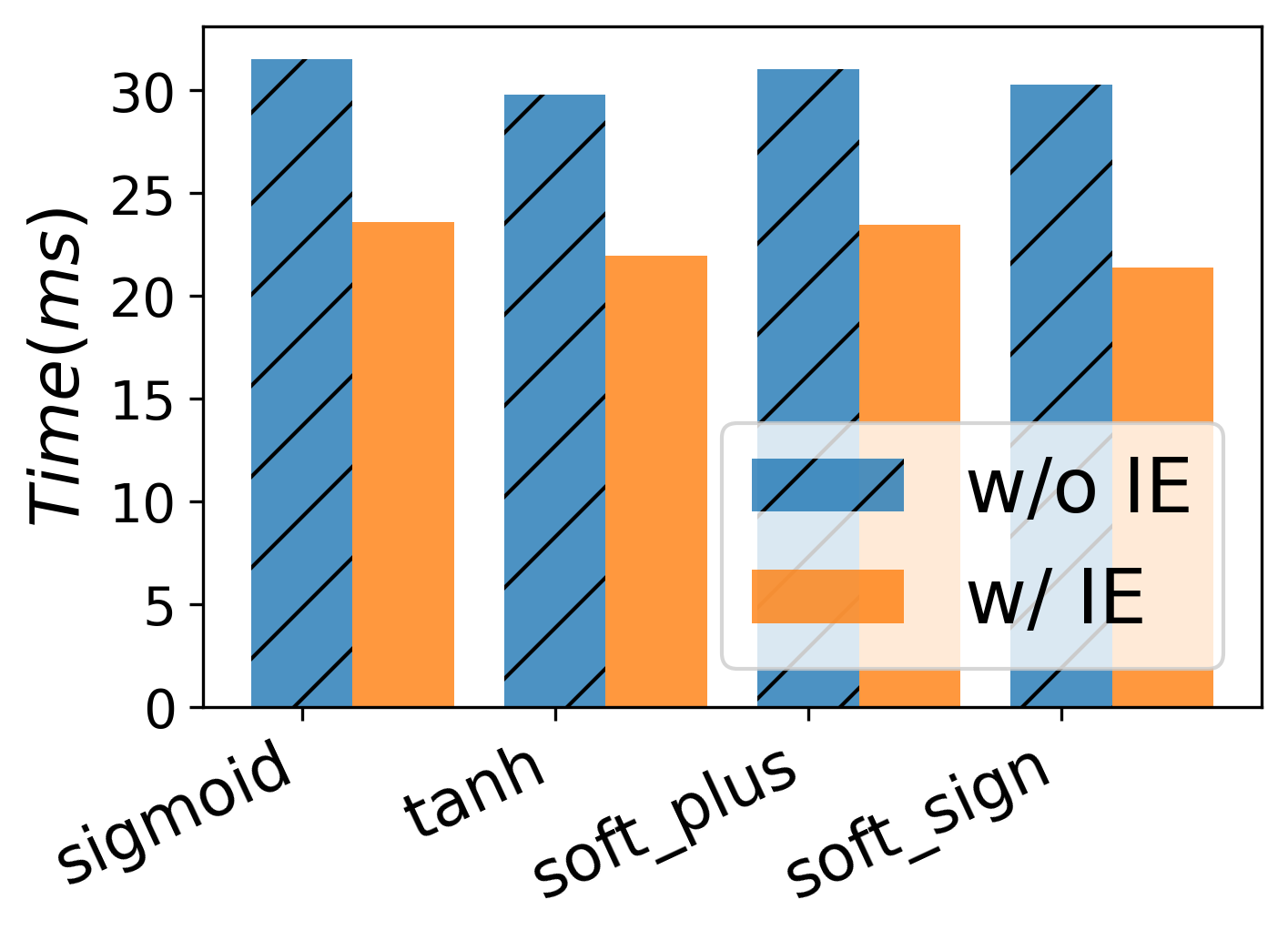
Independence and parallelism. We adopt two types of optimizations to accelerate the online phase performance: 1) Independent evaluation of $\times$ and $>$ : As we have discussed in Section 4.3, it is independent to perform the comparisons and to compute $x$ to the $k$ -th power. We evaluate the speedup on PrivPy by running them independently⁴⁴ 4 MP-SPDZ does not support customized multi-threading in its user-level language so we do not adopt this optimization.. Figure 2(a) shows the performance results with/without independent evaluation. We can see the optimization provides a $1.3-1.4\times$ speedup even on small $100$ -dimensional input.

2) Concurrency on large inputs: Figure 2(b) shows the performance with varied numbers of threads on $10^{6}$ input. We observe good speedup up to $10$ threads (about $4\times$ speedup comparing with the single-thread) for all four functions we evaluate. Using more than 10 threads decreases performance as given the vector size, cost of threading overweights the speedup.

7.3. Accuracy

Accuracy against the baseline. We compute the soft relative distance (SRD in Section 3) on each of the 10,000 input samples. We see a large variation of SRDs on different functions, and Figure 3 shows the cumulative distribution functions (CDFs) of the SRDs on each function for both the baseline and NFGen.

We observe the following: 1) 100% of the SRD of all 10k samples are under $10^{-3}$ (the target $\epsilon$ ), ranging between $10^{-12}$ and $10^{-3}$ , as expected. 2) In comparison, the baseline shows diverse errors across functions. The $Cauchy\_dis$ is very accurate as it is just a $\frac{1}{x}$ (NFGen falls back to direct evaluation in this case). However, in some functions, the baseline shows errors way exceeding the $10^{-3}$ limit (dashed vertical line in Figure 3) on over 10% samples (Function $Bs\_dis$ has 100% and $tanh$ has more than 35%). There are two reasons: precision loss due to concatenating multiple non-linear functions and errors due to overflow/underflow. 3) Baseline has a larger percentage of samples with smaller errors (e.g. $<10^{-9}$ ) than NFGen. This is as expected too: NFGen is based on a regression model to approximate, while baseline is a direct computation. However, we believe the predictable accuracy is more important than sometimes getting smaller errors.

Errors due to overflows/underflows. When the evaluation of $F(x)$ uses an intermediate result in a large range, like $e^{x}$ , it overflows given an $x$ with $|x|>\ln{2^{(96-48-1)}}\approx 33.2$ in MP-SPDZ with $\langle 96,48\rangle$ -FXP. The top two rows in Figure 4 plot SRD vs. $x$ value for the baselines, and show the overflow cases, where the SRD can exceed $10^{5}$ , even if the range of $F(x)$ is perfectly representable. In comparison, the bottom two rows in Figure 4 show that SRDs are less than $10^{-3}$ in NFGen. It also uncovers that NFGen has larger SRD when $F(x)$ is close to zero, as the accuracy of polynomial approximation are constrained by the limited resolution of FXP.

Error accumulation. The error accumulation problem widely exists in scientific computing (Atkinson and Han 2005), even with double precision numbers. Using FXP makes the problem worse, especially when the calculation of the target functions has many steps. As NFGen approximate the entire $F(x)$ in one shot, it does not accumulate errors.

We take the $Bs\_dis$ function (Row 5 in Table 2), whose calculation has four steps, as an example. 1) $x_{11}\leftarrow\sqrt{x};\,x_{12}\leftarrow\frac{1}{x}$ ; 2) $x_{2}\leftarrow\sqrt{x_{12}}$ ; 3) $x_{3}\leftarrow\phi(\frac{x_{11}-x_{2}}{\gamma})$ and 4) $x_{4}\leftarrow(\frac{x_{11}+x_{2}}{2\gamma*x})*x_{3}$ . Using 10k $\hat{x}$ samples, we compute the SRD after each step, and plot the CDF in Figure 5 (left). We can see that although the first two steps results in negligible SRD that is smaller than $10^{-10}$ , more samples starts to show larger SRD after steps 3 and 4. After step 4, only less than half of the samples meet the accuracy requirement of $10^{-3}$ . Figure 5 (right) shows the evaluation results, and we find obvious inaccuracies for $\hat{x}\in[0.054,18]$ , without overflow or underflow. In comparison, NFGen successfully limits the error below $3.8\times 10^{-4}$ using $\hat{p}_{5}^{11}$ .

Accuracy loss in secret sharing. The secret sharing and reconstruction processes in MPC platforms may introduce extra inaccuracies as they approximate each real value in fixed-point shares (Catrina and Saxena 2010; Mohassel and Zhang 2017) (we call it secret sharing reconstruction error (SSRE)). For example, we observe that the value of exactly $1\times 10^{-14}$ , after secret sharing and reconstruction, may become $1.06581\times 10^{-14}$ . This SSRE also adds inaccuracy to the final evaluation result. To quantify the contribution of SSRE, we compare the SRD using real MPC to our simulated FXP (without SSRE). Table 3 shows the comparison (* highlights cases with different results). We can see that SSRE does increase the inaccuracy, but the contribution is small comparing to other sources of inaccuracy.

Table 3. Secret Sharing Reconstruction Loss

	Simulation		Secret Sharing
	Max( $\times 10^{-4}$ )	Mean( $\times 10^{-5}$ )	Max( $\times 10^{-4}$ )	Mean( $\times 10^{-5}$ )
tanh	$8.06$	$3.88$	$8.06$	$3.88$
soft_plus^∗	$7.67$	$2.94$	$8.00$	$2.98$
sigmoid	$3.98$	$1.87$	$3.98$	$1.87$
elu	$8.50$	$12.87$	$8.50$	$12.87$
selu	$5.24$	$1.94$	$5.24$	$1.94$
gelu	$8.79$	$6.11$	$8.79$	$6.11$
isru	$8.61$	$28.18$	$8.61$	$28.18$
normal_dis^∗	$3.40$	$1.01$	$10.49$	$2.53$
gamms_dis	$8.80$	$3.11$	$8.80$	$3.11$
chi_square	$7.27$	$10.70$	$7.50$	$10.70$
exp_dis	$7.39$	$19.76$	$7.39$	$19.77$
log_dis	$4.24$	$3.28$	$4.24$	$3.28$
bs_dis^∗	$5.96$	$1.98$	$6.91$	$1.97$

Accuracy with different FXP widths. Many MPC platforms offer configurable $\langle n,f\rangle$ for FXP numbers. While reducing $n$ saves computation cost, a small $n$ limits the input domain for both baseline methods and NFGen, because we need to represent all inputs, intermediate results and outputs with the number of bits. We conduct experiments with $n$ ranging from 32 to 128 and compare the supported $\hat{x}$ domain between the baseline and NFGen and summarize the results in Table 4.

We observe: 1) As $n$ gets smaller, the ranges shrink for both cases. NFGen supports a much larger domain even for $n=32$ . This is because the baseline domain is severely limited by the range of intermediate results, e.g. $\frac{1}{x}$ overflows when $x$ gets close to zero and $e^{x}$ overflows when $x>\ln{2^{n-f-1}}$ . 2) In contrast, $n$ affects the domain in NFGen in two different ways: a) it directly limits representable $x$ to $|2^{n-f-1}|$ ; b) it limits the representation of $x^{k}$ , forcing us to use only small $k$ values (Column 3). We see that NFGen can automatically adapt to the $n$ settings by reducing the $k$ values to prevent overflows. 3) As expected, a small $k$ limits the accuracy we can achieve. We empirically determine the minimal possible accuracy (both $\hat{0}$ and $\epsilon$ ) when we require $m<1000$ (Column 1), and find that even in the $\langle 32,16\rangle$ setting (i.e. the max representable number is only $2^{15}$ ), we can still maintain an $\epsilon\approx 5\%$ , covering almost the entire representable domain between $-10^{4}$ and $10^{4}$ .

Table 4. Domain Restriction with Data Representation

Config	$F(x)$	$(k,m)$	Origin $D$	Ours $D$
$\langle 128,64\rangle$ $\hat{0}=10^{-6}$ $\epsilon=10^{-4}$	$tanh$	$(6,11)$	$[-44.4,44.4]$	$(-10^{19},10^{19})$
	soft_plus	$(9,9)$	$[-44.4,44.4]$	$(-10^{19},10^{19})$
	Normal_dis	$(6,48)$	$[-9.4,9.4]$	$(-10^{19},10^{19})$
	Bs_dis	$(10,9)$	$[0.0,24.1]$	$(0,10^{19})$
$\langle 96,48\rangle$ $\hat{0}=10^{-6}$ $\epsilon=10^{-3}$	$tanh$	$(6,11)$	$[-33.3,33.3]$	$(-10^{14},10^{14})$
	soft_plus	$(6,11)$	$[-33.3,33.3]$	$(-10^{14},10^{14})$
	Normal_dis	$(10,9)$	$[-8.2,8.2]$	$(-10^{14},10^{14})$
	Bs_dis	$(5,14)$	$[0.1,18.6]$	$(0,10^{14})$
$\langle 64,32\rangle$ $\hat{0}=10^{-5}$ $\epsilon=10^{-3}$	$tanh$	$(5,9)$	$[-22.2,22.2]$	$(-10^{9},10^{9})$
	soft_plus	$(7,9)$	$[-22.2,22.2]$	$(-10^{9},10^{9})$
	Normal_dis	$(10,9)$	$[-6.7,6.7]$	$(-10^{9},10^{9})$
	Bs_dis	$(5,14)$	$[0.1,13.0]$	$(0,10^{9})$
$\langle 32,16\rangle$ $\hat{0}=10^{-2}$ $\epsilon=5\cdot 10^{-2}$	$tanh$	$(4,6)$	$[-11.1,11.1]$	$(-10^{4},10^{4})$
	soft_plus	$(4,6)$	$[-11.1,11.1]$	$(-10^{4},10^{4})$
	Normal_dis	$(4,7)$	$[-4.7,4.7]$	$(-10^{4},10^{4})$
	Bs_dis	$(5,5)$	$[0.1,7.4]$	$(0,10^{4})$

•

* The function range are actually defined by $\hat{0}$ , we set outer range to default constant (e.g., $tanh({\hat{x}})=-1$ for $\forall{\hat{x}}\leq-18.79$ ).

Limitations on accuracy. As NFGen uses approximations, there is no guarantee that it will find a workable polynomial with small $\epsilon$ s. We have shown that when $\epsilon=10^{-3}$ , we can successfully find approximations for all 15 functions. When we set $\epsilon=10^{-4}$ , we fail to find a good $\hat{p}_{k}^{m}$ for $Gamma\_dis$ . If we further limit $\epsilon$ to $10^{-5}$ , six out of the 15 functions fails to fit. However, considering that MPC is mostly employed on data mining applications that do not require high precision, we believe NFGen strikes the right balance between efficiency and predictable accuracy.

7.4. Applied in Real Algorithms

NFGen benefits MPC algorithms mainly in two ways. First, it improves both performance and accuracy for existing MPC algorithms. Second, it allows people to evaluate advanced non-linear functions that we cannot construct with simple built-ins. We use logistic regression (LR) as an example to show the first benefit, and use a series of special functions and the $\chi^{2}$ test to show the second.

Logistic Regression (LR) Accuracy. LR (Bishop and Nasrabadi 2006) is one of the most utilized data mining algorithms, both in plaintext and MPCs. The major challenge for MPC is the slow performance of evaluating sigmoid. Prior projects use a $3$ -piece linear function (Mohassel and Zhang 2017; Mohassel and Rindal 2018), and (Hesamifard et al. 2018) uses single Chebyshev polynomial to approximate the sigmoid. Figure 6 compares the sigmoid function with different approximations.

People argue that the accuracy of sigmoid does not affect the LR accuracy(Mohassel and Zhang 2017; Mohassel and Rindal 2018; Hesamifard et al. 2018). To evaluate this argument, we generate four datasets using Python sklearn’s make_classifiation() method, and use them to train LR models using different approximations. Table 5 reports the LR prediction accuracy. We see that the $3$ -piece approximation can lead to significant LR accuracy loss, while the approximation in (Hesamifard et al. 2018) slightly reduces accuracy. In comparison, NFGen achieves almost the same accuracy as the plaintext result. Thus, sigmoid accuracy does affect LR performance in some cases. NFGen provides an efficient way to evaluate sigmoid with high accuracy, eliminating the need for ad hoc approximations.

Table 5. Performance Analysis of sigmoid

Data setting^∗	Real	NFGen	SecureML (Mohassel and Zhang 2017; Mohassel and Rindal 2018)	(Hesamifard et al. 2018)
$(0.5,3,0.2)$	59.2	59.2	49.2	58.6
$(0.6,3,0.1)$	62.5	62.5	50.8	62.2
$(0.7,3,0.1)$	65.8	65.8	51.4	65.3
$(0.7,4,0.1)$	61.9	61.9	50.0	61.5

•

* The three numbers are arguments class_sep, clusters_per_class and learning_rate passed to the Python sklearn library’s make_classifiation() funtion to generate the dataset.

LR performance. We use 3 real datasets to evaluate LR training and inference time on PrivPy. We omit evaluation on MP-SPDZ as it needs to pre-compile all input data into the program, but the compiler fails on large datasets. Independent of the dataset, we set the $\hat{x}$ domain to $[-10,10]$ , which is a typical setting in practice when the distribution of dataset is unknown (when $x\notin[-10,10]$ , output $0$ or $1$ ). Table 6 shows the results. We can see that NFGen achieves $3.5\times$ to $9.5\times$ speedup in training and $1.8\times$ to $2.3\times$ speedup for inference using $\hat{p}_{8}^{6}$ and with same Accuracy as plaintext LR.

Table 6. Logistic Regression Speedups

Dataset	Method	Train(sec)	Test(sec)
[2pt] Adult (Kohavi et al. 1996) [2pt]( $48,842\times 65$ )	PrivPy	413.1	1.8
[2pt] Adult (Kohavi et al. 1996) [2pt]( $48,842\times 65$ )	NFGen	43.6 / $9.5\times$	0.8 / $2.3\times$
[2pt] Bank (Moro et al. 2014) ( $41,188\times 63$ )	PrivPy	72.8	1.6
[2pt] Bank (Moro et al. 2014) ( $41,188\times 63$ )	NFGen	20.4 / $3.6\times$	0.8 / $2.0\times$
[2pt] Branch (SHKADAREVICH 2021) ( $400,000\times 480$ )	PrivPy	703.8	12.2
[2pt] Branch (SHKADAREVICH 2021) ( $400,000\times 480$ )	NFGen	199.9 / $3.5\times$	6.9 / $1.8\times$

Table 7. Special Functions Demonstration

Target Function	Parameter	$(k,m)$	$T_{\text{Fit}}$ (sec)
$\gamma(x,z)=\int_{0}^{x}t^{z-1}e^{t}\,dt$ , $x\in[0,15]$	$z=1$	(6, 4)	1.1
	$z=2$	(5, 6)	1.6
	$z=3$	(6, 6)	2.0
$\Gamma(x,z)=\int_{x}^{\infty}t^{z-1}e^{t}\,dt$ , $x\in[0,10]$	$z=1$	(6, 6)	1.1
	$z=2$	(8, 4)	1.1
	$z=3$	(7, 4)	1.2
$erf(x)=\frac{2}{\sqrt{\pi}}\int_{0}^{x}e^{-t^{2}}\,dt$ , $x\in[0,5]$	NA	(4, 6)	0.8
$\Phi(x)=\frac{2}{\sqrt{2\pi}}\int_{0}^{x}e^{\frac{-t^{2}}{2}}\,dt$ , $x\in[-5,5]$	NA	(8, 6)	1.2

Hard-to-implement functions. A big problem MPC practitioners face is how to implement some commonly-used but hard-to-implement functions, such as $\gamma{(x)}$ , $\Gamma{(x)}$ and $\Phi{(x)}$ . These functions are defined as integrals, and it takes much mathematical skills to approximate them using the limited operators in MPC (and impossible sometimes). NFGen naturally solves the problem for all Lipschitz continuous functions as long as there is a plaintext implementation available. We demonstrate $8$ hard-to-implement functions in Table 7. We see that like other functions, it only takes about $1$ - $2$ seconds to generate the approximation and achieve small $k$ and $m$ meeting the same accuracy requirement.

The $\chi^{2}$ test on real datasets. $\chi^{2}$ test (Mendenhall et al. 2012) is a classic statistical method. Unfortunately, the $p$ value from $\chi^{2}$ test depends on the $\gamma$ and $\Gamma$ functions in Table 7, as $p=1-\frac{\gamma(\frac{k}{2},\frac{x}{2})}{\Gamma(\frac{k}{2})}$ , where $\frac{\gamma(\frac{k}{2},\frac{x}{2})}{\Gamma(\frac{k}{2})}$ is the CDF of $\chi^{2}$ distribution, $x$ is the statistical value and $k$ is the degree-of-freedom (Dof) parameter that is typically set to the number of classes minus 1. No current MPC framework supports $\chi^{2}$ test yet, to our knowledge. We show that we can easily implement $\chi^{2}$ test with NFGen on real datasets. The datasets contain features of a patient with certain diseases, and as a typical task in medical research, we use $\chi^{2}$ test to determine whether the probability of a disease is correlated to a feature. Table 8 shows that we can evaluate cases with different Dofs, and achieve the same result as in plaintext (with 3 significant digits).

Table 8.

\chi^{2}

Test using Real Datasets

Dataset	Feature	Dof	$(k,m)$	Time(sec)
Cervical (Machmud et al. 2016) [2pt]( $72\times 20$ ) $5$ features for demo	Sexual behavior	5	$(6,11)$	13.8
	Eating behavior	7	$(5,13)$
	Personal hygine	11	$(5,14)$
	Social support	11	$(5,14)$
	Attitude	6	$(5,11)$
Sepsis (Chicco and Jurman 2020) [2pt]( $110,204\times 3$ )	age	10	$(5,12)$	63.3
	sexual	1	$(5,98)$
	episode number	4	$(5,9)$

7.5. Effectiveness of Design Choices

We conduct an ablation study to evaluate the design choices in NFGen, including the Scaling factor (Algorithm 5), Residual boosting (Algorithm 6) and the Merge stage in Algorithm 1, using the same setting as in Section 7.2, on Rep2k.

Table 9. Ablation Studies

$F(x)$	Metric	NFGen	no merge	no boosting	no scaling
$sigmoid$	$T_{\text{Fit}}$	3.1	2.2	14.0	2.6
	Best $(k,m)$	(7, 10)	(5, 20)	(7, 10)	(7, 12)
	Failures	0	0	1	0
soft_plus	$T_{\text{Fit}}$	2.7	1.8	14.1	2.0
	Best $(k,m)$	(7, 4)	(4, 30)	(7, 4)	(4, 9)
	Failures	0	0	1	0
$selu$	$T_{\text{Fit}}$	1.3	0.9	1.2	36.0
	Best $(k,m)$	(8, 9)	(6, 14)	(8, 9)	(6, 12)
	Failures	0	0	0	3
Gamma_dis	$T_{\text{Fit}}$	4.3	1.1	40.8	1.2
	Best $(k,m)$	(7, 21)	(5, 35)	NA	(5, 26)
	Failures	0	0	7	0

We evaluate each technique on four functions, and Table 9 summarizes the result. We measure three metrics on each ablation case: 1) $T_{\text{Fit}}$ is the runtime of Algorithm 1; 2) Best $(k,m)$ is the best-performance $\hat{p}_{k}^{m}$ we find; 3) Failures count the number of cases where we do not find a feasible $\hat{p}_{k}^{m}$ for $k$ with $m<m_{max}$ .

Key observations include: 1) Though each technique takes extra pre-computation time, the overhead is less than 1 second per technique. However, without them some functions are even slower to fit, e.g. $selu$ w/o scaling and $Gamma\_dis$ w/o residual boosting are both slower because some otherwise possible $\hat{p}_{k}^{m}$ will not pass the check and results in more searching steps. 2) The merge step significantly reduces $m$ , as the splitting strategy often unnecessarily increases the number of pieces. 3) Failures are more often if we remove residual boosting or scaling, showing that they effectively make some approximation possible by remedying inaccuracies introduced by the FLP-FXP conversion.

8. Conclusion and Future Work

Creating general-purpose MPC platforms is analogous to creating a new computation system from scratch using MPC primitives instead of instructions. Non-linear function evaluation, akin to plaintext numeric libraries, is one of these systems’ foundations. Prior approaches either naively attempted to reuse plaintext algorithms that resulted in erroneous results and/or slow performance, or developed ad hoc approximations that were tightly coupled with either specific functions or MPC platforms. Neither method possesses the generality or performance necessary to serve as a viable foundation. NFGen is, to our knowledge, the first attempt for a generic solution. We can accurately approximate general non-linear functions using piecewise polynomials by properly handling FXP and FLP operations. We achieve portability across multiple MPC systems and protocols by utilizing code generation and profiler-based performance prediction. Extensive evaluations verify our approach’s effectiveness, accuracy, and generality.

As future work, we are going to support more MPC platforms, explore approximation algorithms with stronger theoretical guarantees, as well as support the evaluation of multi-dimensional non-linear functions.

Acknowledgements

We thank Menghua Cao and Zhilong Chen for insightful discussions during the design of NFGen. We thank Yuanxi Dai and Xinze Li for their assistance with the security analysis. We thank Xiang Wang and Haoqing He for their help during the implementations.

This work is supported in part by the National Natural Science Foundation of China (NSFC) Grant 71872094 and gift funds from Nanjing Turing AI Institute.

References

(1)
876 (2019) 2019. IEEE Standard for Floating-Point Arithmetic. IEEE Std 754-2019 (Revision of IEEE 754-2008) (2019), 1–84. https://doi.org/10.1109/IEEESTD.2019.8766229
Aliasgari et al. (2013) Mehrdad Aliasgari, Marina Blanton, Yihua Zhang, and Aaron Steele. 2013. Secure Computation on Floating Point Numbers. In The Network and Distributed System Security Symposium (NDSS).
Atkinson and Han (2005) Kendall Atkinson and Weimin Han. 2005. Theoretical Numerical Analysis. Vol. 39. Springer.
Beaver (1991) Donald Beaver. 1991. Efficient Multiparty Protocols using Circuit Randomization. In Annual International Cryptology Conference. Springer.
Birnbaum and Saunders (1969) Zygmunt W Birnbaum and Sam C Saunders. 1969. A New Family of Life Distributions. Journal of applied probability (1969).
Bishop and Nasrabadi (2006) Christopher M Bishop and Nasser M Nasrabadi. 2006. Pattern Recognition and Machine Learning, Chapter 4.3.4. Springer.
Bogdanov et al. (2008) Dan Bogdanov, Sven Laur, and Jan Willemson. 2008. Sharemind: A Framework for Fast Privacy-preserving Computations. In European Symposium on Research in Computer Security. Springer.
Boura (2018) Chillotti Ilaria Gama Nicolas Jetchev Dimitar Peceny Stanislav Petric Alexander Boura, Christina. 2018. High-Precision Privacy-Preserving Real-Valued Function Evaluation. In International Conference on Financial Cryptography and Data Security (FC).
Canetti (2000) Ran Canetti. 2000. Security and Composition of Multiparty Cryptographic Protocols. Journal of CRYPTOLOGY (2000).
Canetti (2001) Ran Canetti. 2001. Universally Composable Security: A new Paradigm for Cryptographic Protocols. In IEEE Symposium on Foundations of Computer Science (FOCS). IEEE.
Catrina and Saxena (2010) Octavian Catrina and Amitabh Saxena. 2010. Secure Computation with Fixed-point Numbers. In International Conference on Financial Cryptography and Data Security (FC). Springer.
Chicco and Jurman (2020) Davide Chicco and Giuseppe Jurman. 2020. Survival Prediction of Patients with Sepsis from Age, Sex, and Septic Episode Number Alone. Scientific reports (2020).
Cramer et al. (2018) Ronald Cramer, Ivan Damgård, Daniel Escudero, Peter Scholl, and Chaoping Xing. 2018. SPD $\mathbb{Z}_{2^{k}}$ : Efficient MPC mod $2^{k}$ for Dishonest Majority. In Advances in Cryptology—Crypto.
Dalskov et al. (2020) Anders Dalskov, Daniel Escudero, and Marcel Keller. 2020. Secure Evaluation of Quantized Neural Networks. Proceedings on Privacy Enhancing Technologies (PET) (2020).
Damgård et al. (2019) Ivan Damgård, Daniel Escudero, Tore Frederiksen, Marcel Keller, Peter Scholl, and Nikolaj Volgushev. 2019. New Primitives for Actively-secure MPC over Rings with Applications to Private Machine Learning. In IEEE Symposium on Security and Privacy (S&P). IEEE.
Damgård et al. (2006) Ivan Damgård, Matthias Fitzi, Eike Kiltz, Jesper Buus Nielsen, and Tomas Toft. 2006. Unconditionally secure constant-rounds multi-party computation for equality, comparison, bits and exponentiation. In Theory of Cryptography Conference (TCC). Springer.
Demmler et al. (2015) Daniel Demmler, Thomas Schneider, and Michael Zohner. 2015. ABY-A framework for Efficient Mixed-protocol Secure Two-party Computation.. In The Network and Distributed System Security Symposium (NDSS).
Fan et al. (2021) Xiaoyu Fan, Guosai Wang, Kun Chen, Xu He, and Wei Xu. 2021. PPCA: Privacy-preserving Principal Component Analysis using Secure Multiparty Computation (mpc). arXiv preprint arXiv:2105.07612 (2021).
Hamada et al. (2014) Koki Hamada, Dai Ikarashi, Koji Chida, and Katsumi Takahashi. 2014. Oblivious radix sort: An efficient sorting algorithm for practical secure multi-party computation. Cryptology ePrint Archive (2014).
Han et al. (2020) Kyoohyung Han, Jinhyuck Jeong, Jung Hoon Sohn, and Yongha Son. 2020. Efficient Privacy Preserving Logistic Regression Inference and Training. Cryptology ePrint Archive (2020).
Hastings et al. (2019) Marcella Hastings, Brett Hemenway, Daniel Noble, and Steve Zdancewic. 2019. SoK: General Purpose Compilers for Secure Multi-party Computation. In IEEE Symposium on Security and Privacy (S&P). IEEE.
Hesamifard et al. (2018) Ehsan Hesamifard, Hassan Takabi, Mehdi Ghasemi, and Rebecca N Wright. 2018. Privacy-preserving Machine Learning as a Service. Proceedings on Privacy Enhancing Technologies (PET) (2018).
Keller (2020) Marcel Keller. 2020. MP-SPDZ: A Versatile Framework for Multi-party Computation. In ACM SIGSAC Conference on Computer and Communications Security (CCS).
Keller and Scholl (2014) Marcel Keller and Peter Scholl. 2014. Efficient, oblivious data structures for MPC. In International Conference on the Theory and Application of Cryptology and Information Security (ASIACRYPT). Springer.
Klambauer et al. (2017) Günter Klambauer, Thomas Unterthiner, Andreas Mayr, and Sepp Hochreiter. 2017. Self-normalizing Neural Networks. Advances in neural information processing systems (NIPS) 30 (2017).
Knott et al. (2021) Brian Knott, Shobha Venkataraman, Awni Hannun, Shubho Sengupta, Mark Ibrahim, and Laurens van der Maaten. 2021. CrypTen: Secure Multi-party Computation Meets Machine Learning. Advances in Neural Information Processing Systems (NIPS) (2021).
Kohavi et al. (1996) Ron Kohavi et al. 1996. Scaling up the Accuracy of Naive-bayes Alassifiers: A Decision-tree Hybrid.. In ACM SIGKDD International Conference on Knowledge Discovery & Data Mining (KDD).
learn Documentation (2011) The Scikit learn Documentation. 2011. Polynomial regression: extending linear models with basis functions. https://scikit-learn.org/stable/modules/linear_model.html. (2011).
Li and Xu (2019) Yi Li and Wei Xu. 2019. PrivPy: General and Scalable Privacy-preserving Data Mining. In ACM SIGKDD International Conference on Knowledge Discovery & Data Mining (KDD).
Lindell and Nof (2017) Yehuda Lindell and Ariel Nof. 2017. A Framework for Constructing Fast MPC over Arithmetic Circuits with Malicious Adversaries and an Honest-majority. In ACM SIGSAC Conference on Computer and Communications Security (CCS).
Lindell and Pinkas (2000) Yehuda Lindell and Benny Pinkas. 2000. Privacy Preserving Data Mining. In Annual International Cryptology Conference. Springer.
Lu et al. (2019) Donghang Lu, Thomas Yurek, Samarth Kulshreshtha, Rahul Govind, Aniket Kate, and Andrew Miller. 2019. Honeybadgermpc and asynchromix: Practical asynchronous mpc and its application to anonymous communication. In ACM SIGSAC Conference on Computer and Communications Security (CCS).
Machmud et al. (2016) Rizanda Machmud, Adi Wijaya, et al. 2016. Behavior Determinant Based Cervical Cancer Early Detection with Machine Learning Algorithm. Advanced Science Letters (2016).
MathWorld (2015) Wolfram MathWorld. 2015. Lagrange interpolating polynomial. (2015).
Mendenhall et al. (2012) William Mendenhall, Robert J Beaver, and Barbara M Beaver. 2012. Introduction to Probability and Statistics, Chapter 14. Cengage Learning.
Mohassel and Rindal (2018) Payman Mohassel and Peter Rindal. 2018. ABY3: A Mixed Protocol Framework for Machine Learning. In ACM SIGSAC conference on computer and communications security (CCS).
Mohassel and Zhang (2017) Payman Mohassel and Yupeng Zhang. 2017. SecureML: A System for Scalable Privacy-preserving Machine Learning. In IEEE Symposium on Security and Privacy (S&P). IEEE.
Moro et al. (2014) Sérgio Moro, Paulo Cortez, and Paulo Rita. 2014. A Data-driven Approach to Predict the Success of Bank Telemarketing. Decision Support Systems (2014).
Rathee et al. (2021) Deevashwer Rathee, Mayank Rathee, Rahul Kranti Kiran Goli, Divya Gupta, Rahul Sharma, Nishanth Chandran, and Aseem Rastogi. 2021. SIRNN: A Math Library for Secure RNN Inference. In IEEE Symposium on Security and Privacy (S&P). IEEE.
SHKADAREVICH (2021) DMITRY SHKADAREVICH. 2021. Branch prediction Binary Classification Dataset. https://www.kaggle.com/datasets/dmitryshkadarevich/branch-prediction. (2021).
Tan et al. (2021) Sijun Tan, Brian Knott, Yuan Tian, and David J Wu. 2021. CryptGPU: Fast Privacy-preserving Machine Learning on the GPU. In IEEE Symposium on Security and Privacy (S&P). IEEE.
Trefethen (2019) Lloyd N Trefethen. 2019. Approximation Theory and Approximation Practice, Extended Edition. Society for Industrial and Applied Mathematics (SIAM).

Appendix A Analysis of Algorithm

A.1. Maximum SRD Analysis for Section 3

We prove the upper-bound of the real maximum soft relative distance between the piecewise polynomial $\hat{p}_{k}^{m}$ and the target Lipschitz continuous $F(x)$ over domain ${\hat{x}}\in[a,b]$ in this section.

Theorem A.1 (Upper-bound of maximum soft relative distance between approximation and target function).

By constraining the maximum soft relative distance (Eq 1) over sample set $\mathbf{{\hat{x}}}=\{{\hat{x}}_{1},...,{\hat{x}}_{i},...,{\hat{x}}_{N}\}$ as Eq 2, where the sampling interval $r=\frac{b-a}{N}$ , there exist constant $C$ , such that the piecewise polynomial $\hat{p}_{k}^{m}$ and target Lipschitz continuous function $F(x)$ satisfy:

\max_{{\hat{x}}\in[a,b]}|F({\hat{x}})-\text{{$\hat{p}_{k}^{m}$} }({\hat{x}})|_{d}\leq\begin{cases}\frac{C\cdot r}{|F({\hat{x}})|}+1,&|F({\hat{x}})|>\hat{0}\\ C\cdot r+\epsilon,&|F({\hat{x}})|\leq\hat{0}\end{cases}

Proof.

As $F(x)$ and piecewise polynomial $\hat{p}_{k}^{m}$ $(x)$ (refer to $p(x)$ in the following proof for simplicity) are both Lipschitz continuous, there exist Lipschitz constants $C_{F}$ and $C_{p}$ that for any interval $[{\hat{x}}_{i},{\hat{x}}_{i+1}]$ , where ${\hat{x}}_{i}\,\text{and}\,{\hat{x}}_{i+1}\,\in\mathbf{{\hat{x}}}$ , $|{\hat{x}}_{i+1}-{\hat{x}}_{i}|=r$ are successive sample points, we have:

(5)			$\displaystyle\|F({\hat{x}})-F({\hat{x}}_{i})\|\leq C_{F}\cdot\|{\hat{x}}-{\hat{x}}_{i}\|\leq C_{F}\cdot r,$
(5)			$\displaystyle\|p({\hat{x}})-p({\hat{x}}_{i})\|\leq C_{p}\cdot\|{\hat{x}}-{\hat{x}}_{i}\|\leq C_{p}\cdot r,$

for $\forall{\hat{x}}\in[{\hat{x}}_{i},{\hat{x}}_{i+1}]$ .

As the accuracy constraint (Eq 2) satisfies on sample set $\mathbf{{\hat{x}}}$ , we have:

(6)

\max_{{\hat{x}}\in\mathbf{{\hat{x}}}}|F({\hat{x}})-p({\hat{x}})|_{d}\leq\epsilon.

Thus, the absolute distance $|F({\hat{x}})-p({\hat{x}})|$ , $\forall{\hat{x}}\in[{\hat{x}}_{i},{\hat{x}}_{i+1}]$ satisfies:

(7)			$\displaystyle\|F({\hat{x}})-p({\hat{x}})\|$
			$\displaystyle=\|F({\hat{x}})+F({\hat{x}}_{i})-F({\hat{x}}_{i})+p({\hat{x}}_{i})-p({\hat{x}}_{i})-p({\hat{x}})\|$
			$\displaystyle\leq\|F({\hat{x}})-F({\hat{x}}_{i})\|+\|F({\hat{x}}_{i})-p({\hat{x}}_{i})\|+\|p({\hat{x}}_{i})-p({\hat{x}})\|$
			$\displaystyle\leq C_{F}\cdot r+C_{p}\cdot r+\|F({\hat{x}}_{i})-p({\hat{x}}_{i})\|$

1) When $|F({\hat{x}}_{i})|>\hat{0}$ , we have $|F({\hat{x}}_{i})-p({\hat{x}}_{i})|\leq\epsilon\cdot|F({\hat{x}}_{i})|$ (Eq 1). As $|F({\hat{x}})-F({\hat{x}}_{i})|\leq C_{F}\cdot r$ holds (Eq 5), then $|F({\hat{x}}_{i})|\leq C_{F}\cdot r+|F({\hat{x}})|$ , thus from Eq 7, we have:

	$\displaystyle\|F({\hat{x}})-p({\hat{x}})\|$	$\displaystyle\leq C_{F}\cdot r+C_{p}\cdot r+\epsilon\cdot\|F({\hat{x}}_{i})\|$
		$\displaystyle\leq C_{F}\cdot r+C_{p}\cdot r+\epsilon\cdot(C_{F}\cdot r+\|F({\hat{x}})\|)$
		$\displaystyle\leq(C_{F}+C_{p}+\epsilon\cdot C_{F})\cdot r+\epsilon\cdot\|F({\hat{x}})\|,$

Let $C=C_{F}+C_{p}+\epsilon\cdot C_{F}$ , when $|F({\hat{x}})|>\hat{0}$ , we have:

(8)

\displaystyle|F({\hat{x}})-p({\hat{x}})|_{d}

\displaystyle=\frac{|F({\hat{x}})-p({\hat{x}})|}{F({\hat{x}})}\leq\frac{C\cdot r}{|F({\hat{x}})|}+\epsilon,

otherwise:

(9)

\displaystyle|F({\hat{x}})-p({\hat{x}})|_{d}

\displaystyle=|F({\hat{x}})-p({\hat{x}})|\leq C\cdot r.

2) When $|F({\hat{x}}_{i})|\leq\hat{0}$ , we can bound the range of $|F({\hat{x}})|$ as:

	$\displaystyle\|F({\hat{x}})\|$	$\displaystyle\leq C_{F}\cdot r+\|F({\hat{x}}_{i})\|$
		$\displaystyle\leq C_{F}\cdot r+\hat{0}<C_{F}\cdot r+\epsilon,$

and we have $|F({\hat{x}}_{i})-p({\hat{x}}_{i})|\leq\epsilon$ , combining with Eq 7:

|F({\hat{x}})-p({\hat{x}})|\leq C_{F}\cdot r+C_{p}\cdot r+\epsilon.

Let $C=C_{F}+C_{\mathcal{P}}$ , when $|F({\hat{x}})|>\hat{0}$ , we have:

(10)	$\displaystyle\|F({\hat{x}})-p({\hat{x}})\|_{d}$	$\displaystyle=\frac{\|F({\hat{x}})-p({\hat{x}})\|}{\|F({\hat{x}})\|}$
		$\displaystyle\leq\frac{(C_{F}+C_{\mathcal{P}})\cdot r}{\|F({\hat{x}})\|}+\frac{\epsilon}{\|F({\hat{x}})\|}$
		$\displaystyle\leq\frac{(C_{F}+C_{\mathcal{P}})\cdot r}{\|F({\hat{x}})\|}+\frac{\epsilon}{C_{F}\cdot r+\epsilon}$
		$\displaystyle\leq\frac{C\cdot r}{\|F({\hat{x}})\|}+1,$

otherwise:

(11)

\displaystyle|F({\hat{x}})-p({\hat{x}})|_{d}=|F({\hat{x}})-p({\hat{x}})|\leq C\cdot r+\epsilon.

Combining Eq 8,9,10,11, we prove the result in Theorem A.1. ∎

A.2. Effectiveness of Simulated ${\hat{x}}$ through $\mathsf{FLPsimFXP}$ (Algorithm 4)

For all possible FLP encoded input $x\in\mathbb{R}$ , the return value $x^{\prime}=\mathsf{FLPsimFXP}(x,n,f)$ can be represented in $\langle n,f\rangle$ -FXP.

$\forall x\in\mathbb{R}$ , if it returns in the first two steps of $\mathsf{FLPsimFXP}$ (Algorithm 4), then it is obvious. Otherwise, it does not return in the first two steps of $\mathsf{FLPsimFXP}$ , it satisfies that:

(12)

2^{-f}\leq|x|\leq{2^{n-f-1}}

As $\mathsf{round}_{2}(x,f)$ rounds-off all the bits beyond $f$ bit after decimal point to $0$ , we have that: $\bar{x}=\mathsf{round}_{2}(x,f)\cdot 2^{f}$ is equivalent to an integer as all bits after the decimal point is $0$ .

As $|\bar{x}|\leq|x|\cdot 2^{f}$ , the range of $|\bar{x}|$ satisfies $0\leq|\bar{x}|\leq 2^{n-1}$ . Thus, there exist an $n$ -bit integer $\bar{x}$ representing $x^{\prime}$ where $x^{\prime}=\bar{x}\cdot 2^{-f}$ , which is representable in $\langle n,f\rangle$ -FXP number format.

A.3. Complexity Analysis of OPPE (Algorithm7)

Theorem A.2 (Complexity of OPPE Algorithm).

The $\mathsf{\times}$ ’s complexity is $O(km+k\log{k})$ and $\mathsf{>}$ ’s complexity is $O(m)$ .

Proof.

In OPPE Algorithm7, there are totally $m$ $\mathsf{>}$ ’s, in Line1. Thus the complexity of $\mathsf{>}$ ’s is quite straightforward, which is $O(m)$ .

For complexity of $\mathsf{\times}$ ’s, which comes from three parts: 1) Line 3-6, $(2km)$ plaintext-ciphertext $\mathsf{\times}$ ’s; 2) Line 8, $(2k)$ ciphertext $\mathsf{\times}$ ’s and 3) Line 7, from CalculateKx function. In CalculateKx function, there are totally $(\lfloor\log{k}\rfloor+1)$ rounds of $\mathsf{\times}$ ’s. In each $i$ round, there are $((k+1)-2^{i-1})$ ciphertext $\mathsf{\times}$ ’s, $i=1,...,\lfloor\log{k}\rfloor+1$ . Suppose there are totally $n$ $\mathsf{\times}$ ’s in CalculateKx, we have

(13)	$\displaystyle n$	$\displaystyle=\sum_{i=1}^{i=\lfloor\log{k}\rfloor+1}{(k+1-2^{i-1})}$
		$\displaystyle=(\lfloor\log{k}\rfloor+1)(k+1)-2^{\lfloor\log{k}\rfloor+1}+1$
		$\displaystyle\approx(k+1)\log{k}-k+2$

As the cost of plaintext-ciphertext $\mathsf{\times}$ is equal or less than ciphertext-ciphertext $\mathsf{\times}$ in most MPC platforms, the complexity of $\mathsf{\times}$ ’s is $O((k+1)\log{k}-k+2+2k+2km)=O(klog{k}+km)$ . ∎

A.4. Obliviousness of OPPE (Algorithm 7)

An oblivious algorithm means that the execution path is independent of the inputs. In multi-party computation, such property refers to a deterministic and data-independent sequence of executing secure operations, like secure oblivious sort algorithm (Hamada et al. 2014) and secure oblivious data access algorithm (Keller and Scholl 2014). The obliviousness property of the OPPE Algorithm 7 is quite straightforward as there are no branches based on the inputs or any variables calculated directly or indirectly from the inputs. Formally, we have

Theorem A.3 (Obliviousness of OPPE Algorithm 7).

With subroutines $\mathsf{ADD},\mathsf{MUL}$ and $\mathsf{GT}$ work as black boxes evaluating secure addition, multiplication and greater-than, the execution path of OPPE Algorithm 7 is independent of the inputs.

Proof sketch. For any two representable input values $(\hat{x},\hat{x^{\prime}})$ , no differences in the evaluation path will be introduced outsides the subroutines ( $\mathsf{ADD},\mathsf{MUL}$ and $\mathsf{GT}$ which work as black boxes).

Appendix B Security Analysis

We adopt the same definitions with Canetti’s work (Canetti 2000) in this section. For completeness, we first introduce the security paradigm for readers not familiar with this area, and then give the security definitions and proof of NFGen’s protocols.

B.1. Formal Security Definition

In the Real-Ideal proof paradigm introduced in (Canetti 2000), two processes ideal and real are defined.

In the Ideal-process, we assume a trusted third party exists, who receives the inputs from all parties, and evaluates the target function $f$ locally and distributes the designated results to each party; the ideal $t$ -limited adversary $\mathcal{A}^{*}$ controls a set of at most $t$ corrupted parties, learns their identities, inputs, internal states, received outputs and can modify their inputs to arbitrary value based on the gathered information.

In the real-process, parties interact with each other according to a protocol $\pi$ in the presence of a real $t$ -limited adversary $\mathcal{A}$ , who controls a set of at most $t$ corrupted parties in some adversarial model (e.g., semi-honest / malicious, adaptive / non-adaptive). At the end of the computation, the real adversary can let the corrupted parties output some arbitrary value.

There are several adversarial models to use. For example, adaptive vs. non-adaptive. To model an adaptive adversary, people introduce an environment identity $\mathcal{Z}$ that can see the inputs, internal states and outputs of all the parties and interacts with the adversary during the evaluation for both ideal and real-processes. On the other hand, to model a non-adaptive adversary, the adversary cannot interact with $\mathcal{Z}$ , nor can it change the member of corrupted parties during the execution.

We define our security in the adaptive model (including both semi-honest and malicious), which is a stronger security definition. Let IDEAL ${}_{f,\mathcal{A}^{*},\mathcal{Z}}$ denote the distribution ensemble of all the parties outputs under any valid security parameter, inputs and randomness in the ideal-process; and let EXEC_π,A,Z denote the same distribution ensemble in the real-process. In the real-ideal paradigm, $\pi$ securely evaluate function $f$ if it emulates the ideal-process in the real-process under any effect of the real adversary $\mathcal{A}$ that can be achieved by some ideal adversary $\mathcal{A}^{*}$ . We formally define the secure evaluation with the following Definition B.1:

Definition B.1 (Secure Evaluation).

Let $f$ be an $n$ -party function and let $\pi$ be a protocol for $n$ parties. We say that protocol $\pi$ adaptively $t$ -securely evaluates $f$ if for any adaptive $t$ -limited real adversary $\mathcal{A}$ and any environment $\mathcal{Z}$ , there exists an adaptive ideal-process adversary $\mathcal{A}^{*}$ whose running time is polynomial in the running time of $\mathcal{A}$ , such that

(14)

{IDEAL}_{f,\mathcal{A}^{*},\mathcal{Z}}\overset{c/s}{\approx}{EXEC}_{\pi,\mathcal{A},\mathcal{Z}},

where $\overset{c/s}{\approx}$ means two distribution ensembles computationally or statistically indistinguishable (suitable for computational-limited or unlimited adversary).

B.2. Security Property Proof of NFGen

In this section, we first briefly introduce the Canetti’s composition theorem (Canetti 2000) and use it to prove the security preserving property of NFGen. Note that the following definitions suit for both semi-honest and malicious adversaries (Canetti 2000).

Secure composition. One commonly used method in developing complex high-level secure protocols for some task is the modular composition (Canetti 2000). We firstly design the high-level protocol by assuming that a series of simple sub-protocols can be carried out securely. Then we design each secure sub-protocol meeting the security guarantee and plug them as subroutines in the high-level protocol. The composition theorem states that, if the high-level protocol can securely evaluate (as defined in Definition B.1) its function with ideal sub-protocols, then the security and functionality maintained by replacing all the ideal sub-protocols into subroutines.

Theorem B.2 (secure composition theorem (Collary12 in (Canetti 2000))).

Let $t<n$ , let $m\in N$ and let $f_{1},...,f_{m}$ be $n$ -party functions. Let $\pi$ be an n-party protocol that adaptively t-securely evaluates $g$ in the $(f_{1},...,f_{m})-$ hybrid model and assumes that no more than one ideal evaluation call is made at each round. Let $\pi_{1},...,\pi_{m}$ be n-party protocols that adaptively t-securely evaluate $f_{1},...,f_{m}$ . Then the protocol $\pi^{\pi_{1},...,\pi_{m}}$ adaptively t-securely evaluates $g$ .

The $(f_{1},...,f_{m})-$ hybrid model means that the joint parties have the access to call ideal functions $f_{1},...,f_{m}$ .

Security-preserving property of NFGen. The generated protocol of NFGen has the property that it guarantees the same security property with three provided subroutines $\mathsf{ADD},\mathsf{MUL}$ and $\mathsf{GT}$ evaluating secure addition, multiplication and greater-than. Formally, it has

Theorem B.3 (Security preserving property of NFGen).

Let $t<n$ , and let $f_{+},f_{\times},f_{>}$ be $n$ -party functions evaluating addition, multiplication and greater-than. Let $\pi_{+},\pi_{\times},\pi_{>}$ be n-party protocols that t-securely evaluate $f_{+},f_{\times},f_{>}$ . Then the protocol $\pi_{OPPE}^{\pi_{+},\pi_{\times},\pi_{>}}$ generated by NFGen t-securely evaluates $\hat{p}_{k}^{m}$ .

Proof sketch. Firstly, the protocol $\pi_{OPPE}$ generated through OPPE Algorithm 7 can securely evaluate $\hat{p}_{k}^{m}$ in the $(f_{+},f_{\times},f_{>})-$ hybrid model. The protocol $\pi_{OPPE}$ can be constructed by replacing subroutines $\mathsf{ADD},\mathsf{MUL}$ and $\mathsf{GT}$ with $f_{+},f_{\times}$ and $f_{>}$ following OPPE Algorithm 7. Since OPPE Algorithm 7 organizes each subroutine $\mathsf{ADD},\mathsf{MUL}$ and $\mathsf{GT}$ sequentially without revealing any information nor introducing any interactions among parties, any cheating behaviors will only happen inside the subroutines. As these subroutines in $\pi_{OPPE}$ are ideal functions $f_{+},f_{\times}$ and $f_{>}$ , thus the real-process distribution ensemble ${EXEC}^{f_{+},f_{\times},f_{>}}_{\pi_{OPPE},\mathcal{A},\mathcal{Z}}$ in the hybrid-model is indistinguishable to the ideal-process distribution ensemble ${IDEAL}_{\hat{p}_{k}^{m},\mathcal{A}^{*},\mathcal{Z}}$ . Then, by the composition theorem B.2, with protocols $\pi_{+},\pi_{\times},\pi_{>}$ that securely evaluate $f_{+},f_{\times}$ and $f_{>}$ , $\pi_{OPPE}$ can securely evaluate $\hat{p}_{k}^{m}$ by replacing each ideal function calls to the corresponding protocols.

Appendix C NFGen Code Examples

In this section, we give a detailed code example to demonstrate the workflow of NFGen, here the selected case is privacy-preserving LR requiring sigmoid.

The NFD config is shown in Code 1, containing the function expression(function), target domain $[a,b]$ (range), accuracy threshold $\epsilon$ and $\hat{0}$ (tol and zero_mask), number representaion $\langle n,f\rangle$ . In this case, it also provide supported operations with profiled time (time_dict) and generated performance model(profiler), these two configurations can also be offered in a separated PPD file. Also, the user can select or offer corresponding code templet(code_templet) and set the output file path(config_file). Then the user can generate specific code by revoke generate_nonlinear_config as Code 3. The generated code is shown in Code block 3, which can be directly executed in MP-SPDZ environment.

⬇

1 import NFGen.CodeTemplet.templet as temp

import NFGen.PerformanceModel.time_ops as to

import sympy as sp

def sigmoid(x):

6 # mpc_exp: lambda x:sp.exp(x)

# mpc_reci: lambda x:1/x, indicating cipher operator.

return 1 * mpc_reci(1 + mpc_exp(-x))

config_sigmoid = { # NFD Config

11 ’function’: sigmoid,

’range’: (-8, 10),

’tol’: 1e-3,

’n’: 96,

’f’: 48,

16 # soft zero.

’zero_mask’: 1e-6,

# Set the value out of range.

’default_values’: (0, 1),

# Supported operations.

21 ’ops’: [’mpc_exp’, ’mpc_reci’, ’mpc_log’, ’mpc_sqrt’],

# SPDZ code templet.

# PrivPy templet use: temp.templet_privpy_cpp.

’code_templet’: temp.templet_spdz,

# Output file.

26 ’config_file’: ’./config_sigmoid.py’,

# PPD part

# Time for basic ops(identify mpc_func operators).

’time_dict’: to.basic_time[’Rep3’],

# Profiler model.

31 ’profiler’: ’../PerformanceModel/Rep3_kmProfiler.pkl’

}

Code Listing 1: NFD & PPD config demo

⬇

1 from NFGen.main import generate_nonlinear_config

# Pass the config and generate code.

generate_nonlinear_config(config_sigmoid)

Code Listing 2: Code generation

⬇

1 @types.vectorize

def sigmoid(x):

"""Version2 of general non linear function.

Args:

6 x (Sfixed): the input secret value.

Returns:

Sfixed: secret f(x).

"""

11 # In user-level mpc file:

# probability trunction acceleration.

program.use_trunc_pr = True

program.use_split(3)

16 # Config of piece-wise polynomial

breaks = [-1009.0, -10.0, -7.5, -5.0, -2.5, -1.25, 0.0,

1.25, 10.0]

coeffA = [[0.0, 0.0, 0.0, 0.0, 0.0, 0.0],

[584022.5019194265, 284883.4701294364, 56450.73475537558,

21 5664.37093087678, 287.16193188632, 5.87319252822],

[1715838.8184591327, 1068788.52768671, 274863.81230151834,

36252.85955923422, 2439.47176809213, 66.71430835583],

[2506924.277852222, 1808567.6009333746, 551644.7862473574,

87996.36476823808, 7267.35497880345, 246.29936351578],

26 [2098737.027154335, 1041805.6678011644, -34419.2181203451,

-140100.88887670645, -37953.67734930042, -3405.3812230294],

[2097139.5017196543, 1054758.5017103767, 29315.2376400353,

-56099.88246721192, 0.0, 0.0],

[2097139.5017196543, 1054758.5017103783, -29315.2376400381,

31 -56099.88246721102, 0.0, 0.0],

[1857186.3089880324, 1582070.1166638373, -437353.1379880485,

60781.5325081042, -4203.393886761, 115.03921274796],

[1.0, 0.0, 0.0, 0.0, 0.0, 0.0]]

scaler = [[1.0, 1.0, 1.0, 1.0, 1.0, 1.0],

36 [2.3842e-07, 2.3842e-07, 2.3842e-07, 2.3842e-07, 2.3842e-07,

2.3842e-07], [2.3842e-07, 2.3842e-07, 2.3842e-07,

2.3842e-07, 2.3842e-07, 2.3842e-07], [2.3842e-07,

2.3842e-07, 2.3842e-07, 2.3842e-07, 2.3842e-07,

2.3842e-07], [2.3842e-07, 2.3842e-07, 2.3842e-07,

41 2.3842e-07, 2.3842e-07, 2.3842e-07], [2.3842e-07,

2.3842e-07, 2.3842e-07, 2.3842e-07, 1.0, 1.0],

[2.3842e-07, 2.3842e-07, 2.3842e-07, 2.3842e-07, 1.0, 1.0],

[2.3842e-07, 2.3842e-07, 2.3842e-07, 2.3842e-07,

2.3842e-07, 2.3842e-07], [1.0, 1.0, 1.0, 1.0, 1.0, 1.0]]

m = len(coeffA)

k = len(coeffA[0])

degree = k-1

51 # Compute the target mask.

comp = sfix.Array(m)

for i in range(m):

comp[i] = (x >= breaks[i])

cipher_index = bb.get_last_one(comp)

# Calculate [1, x, x^2, ..., x^{k}].

pre_muls = floatingpoint.PreOpL(lambda a,b,_:

a * b, [x] * degree)

61 # Compute c_i*x^i*s_i.

poss_res = [0]*m

for i in range(m):

poss_res[i] = coeffA[i][0] * scaler[i][0]

for j in range(degree):

66 poss_res[i] += (coeffA[i][j+1]

* pre_muls[j] * scaler[i][j+1])

# Get result with mask and all possible values.

return sfix.dot_product(cipher_index, poss_res)

Code Listing 3: Generated Code (MP-SPDZ)

⬇

1 bool SS4Runner::sigmoid(const size_type length,

TypeSet::FNumberArr *result,

const TypeSet::FNumberArr *num,

bool use_current_thread) {

check_runner_terminate_status(false);

6 TypeSet::FNUMT *result_x = result->get_x(), *result_x_ = result->get_x_();

const size_type K = 9;

const size_type config_length = length * K;

TypeSet::FNumberArr coeff(config_length);

11 TypeSet::FNumberArr scaler(config_length);

TypeSet::FNumberArr x_items(config_length);

sigmoid_calculateCoeff (length, &coeff, &scaler, num); });

calculateKx(length, &x_items, num, K); });

mul<TypeSet::FNUMT>(config_length, &x_items, &x_items, &coeff);

mul<TypeSet::FNUMT>(config_length, &x_items, &x_items, &scaler);

double *ftmp2 = new double[length];

21 for (int i = 0; i < length; i++) ftmp2[i] = 0.0;

map2numv<double, TypeSet::FNUMT>(ftmp2, length, result);

for (size_type i = 0; i < length; i++) {

for (size_type j = 0; j < K; j++) {

26 result_x[i] += x_items.x[i * K + j];

result_x_[i] += x_items.x_[i * K + j];

}

delete[] ftmp2;

31 return true;

}

bool SS4Runner::sigmoid_calculateCoeff(const size_type length,

TypeSet::FNumberArr *coeff,

36 TypeSet::FNumberArr *scaler,

const TypeSet::FNumberArr *num) {

check_runner_terminate_status(false);

TypeSet::FNUMT *num_x = num->get_x(), *num_x_ = num->get_x_();

41 const size_type M = 7;

const size_type K = 9;

const double Breaks[M] = {-1009.0, -10.0, -5.0, -1.25, 0.0, 1.25, 10.0};

const double CoeffA[M * K] = {0.0, 0.0, 0.0, 0.0, 0.0, 0.0, 0.0, 0.0, 0.0, 2736794.311829414, 2166127.0649512047, 779033.1999940014, 165208.365427917, 22462.75021140543, 1994.81274157933, 112.49785815234, 3.6702035068, 0.05287661137, 2060712.4699856702, 909977.1725834787, -224423.69609669817, -287140.3378066692, -103632.73876614487, -20259.29529210076, -2311.60919005347, -144.85798280994, -3.84685342155, 2097139.5017196543, 1054758.5017103767, 29315.2376400353, -56099.88246721192, 0.0, 0.0, 0.0, 0.0, 0.0, 2097139.5017196543, 1054758.5017103783, -29315.2376400381, -56099.88246721102, 0.0, 0.0, 0.0, 0.0, 0.0, 2020005.5083353834, 1217129.597655899, -113822.68074184433, -88781.97063835277, 35521.12204303316, -6139.86216019294, 574.93708725425, -28.4375893287, 0.58380827441, 1.0, 0.0, 0.0, 0.0, 0.0, 0.0, 0.0, 0.0, 0.0};

const double Scaler[M * K] = {1.0, 1.0, 1.0, 1.0, 1.0, 1.0, 1.0, 1.0, 1.0, 2.3842e-07, 2.3842e-07, 2.3842e-07, 2.3842e-07, 2.3842e-07, 2.3842e-07, 2.3842e-07, 2.3842e-07, 2.3842e-07, 2.3842e-07, 2.3842e-07, 2.3842e-07, 2.3842e-07, 2.3842e-07, 2.3842e-07, 2.3842e-07, 2.3842e-07, 2.3842e-07, 2.3842e-07, 2.3842e-07, 2.3842e-07, 2.3842e-07, 1.0, 1.0, 1.0, 1.0, 1.0, 2.3842e-07, 2.3842e-07, 2.3842e-07, 2.3842e-07, 1.0, 1.0, 1.0, 1.0, 1.0, 2.3842e-07, 2.3842e-07, 2.3842e-07, 2.3842e-07, 2.3842e-07, 2.3842e-07, 2.3842e-07, 2.3842e-07, 2.3842e-07, 1.0, 1.0, 1.0, 1.0, 1.0, 1.0, 1.0, 1.0, 1.0};

// 1. Calculate the corresponding index

// a) Expand num and breaks to outter_comparision.

const size_type expand_length = length * M;

TypeSet::FNumberArr findex_arr(expand_length);

51 outter_gt<double, TypeSet::FNUMT>(Breaks, num, expand_length, &findex_arr);

// b) Compute the target mask

for (size_type i = 0; i < length; i++) {

memcpy(ctmp + i * M, findex_arr + i*M+1, sizeof(TypeSet::FNUMT) * (M - 1));

}

56 sub<TypeSet::FNUMT>(expand_length, &findex_arr, &findex_arr, &ctmp);

// 2. Fetch out target coeff and scaler.

const size_type config_length = length * K;

TypeSet::FNumberArr coeff(config_length);

TypeSet::FNumberArr scaler(config_length);

61 size_type shape1[2] = {length, M};

size_type shape2[2] = {M, K};

inner_product<TypeSet::FNUMT, double>(

&coeff, shape1, shape2, &findex_arr, CoeffA);

inner_product<TypeSet::FNUMT, double>(

66 &scaler, shape1, shape2, &findex_arr, Scaler);

return true;

}

Code Listing 4: Generated Code (PrivPy C++ Code)

⬇

1 @pp.local_import("numpy", "np")

def sigmoid(x):

import pnumpy as pnp

def _calculate_kx(x, k):

6 items = pnp.transpose(pnp.tile(x, (k, 1)))

items[:, 0] = pp.sfixed(1)

shift = 1

while shift < k:

11 items[:, shift:] *= items[:, :len(items[0])-shift]

shift *= 2

return items

def _fetch_index(x, breaks):

16 if isinstance(x, pp.FixedArr):

x = pnp.transpose(pnp.tile(x, (len(breaks), 1)))

breaks = np.tile(breaks, (len(x), 1))

cipher_comp = x >= breaks

21 cipher_index = pnp.util.get_last_one(cipher_comp)

return cipher_index

# same breaks, coeffA and scaler with other generated code.

breaks = np.array(breaks)

coeffA = np.array(coeffA)

scalerA = np.array(scaler)

31 k = int(len(coeffA[0]))

cipher_index = _fetch_index(x, breaks)

coeff = pnp.dot(cipher_index, coeffA)

scaler = pnp.dot(cipher_index, scalerA)

x_items = _calculate_kx(x, k)

36 tmp_res = x_items * coeff

res = pnp.sum(tmp_res * scaler, axis=1)

return res

Code Listing 5: Generated Code (PrivPy Python Code)

Appendix D Full Micro-benchmark Results

Table 10. Micro-benchmark for probability distribution functions

$F(x)$	$\mathcal{S}$	✓	$(k,m)$	$T_{\text{Fit}}$	Communication(MB)			Efficiency(Ms)
$F(x)$	$\mathcal{S}$	✓	$(k,m)$	$T_{\text{Fit}}$	Base	NFGen	Save	Base	NFGen	SpeedUp
$\textit{Normal\_dis}(x)=\frac{e^{-\frac{x^{2}}{2}}}{\sqrt{2\pi}}$ $x\in[-10,+10]$ , $F(x)\in[0.0,0.4]$ Non-linear buildling-blocks: $1$	A	$\times$	(8, 12)	5.2	420	295	30%	67	24	2.8 $\times$
	B	$\times$	(8, 12)	3.6	3	2	45%	4906	156	31.5 $\times$
	C	$\times$	(8, 12)	3.6	7	5	27%	5029	970	5.2 $\times$
	D	$\times$	(8, 12)	3.6	24	23	5%	6588	1846	3.6 $\times$
	E	$\times$	(5, 22)	3.6	257	481	-87%	89740	166328	0.5 $\times$
	F	$\times$	(8, 12)	3.6	249	301	-21%	14908	14861	1.0 $\times$
$\textit{Cauchy\_dis}(x)=\frac{1}{\pi(1+x^{2})}$ $x\in[-40,+40]$ , $F(x)\in[0.0,0.3]$ Non-linear buildling-blocks: $1$	A	✓	(10, 10)	4.4	202	295	-50%	82	26	3.2 $\times$
	B	✓	NA	3.6	1	1	0%	69	71	1.0 $\times$
	C	✓	NA	3.6	2	2	0%	405	403	1.0 $\times$
	D	✓	NA	3.6	8	8	0%	698	689	1.0 $\times$
	E	✓	NA	3.6	50	50	0%	15496	15677	1.0 $\times$
	F	✓	NA	3.6	47	47	0%	2248	2243	1.0 $\times$
$\textit{Gamma\_dis}(x)=\frac{x^{\gamma-1}e^{-x}}{\Gamma(\gamma)}$ $\gamma=0.5$ , $x\in[0.0,50]$ , $F(x)\in[0.0,0.4]$ Non-linear buildling-blocks: $2$	A	$\times$	(7, 19)	5.9	793	393	50%	137	30	4.6 $\times$
	B	$\times$	(7, 21)	4.3	3	2	26%	4624	216	21.4 $\times$
	C	$\times$	(5, 27)	4.3	6	8	-30%	5008	1443	3.5 $\times$
	D	$\times$	(5, 27)	4.3	23	33	-45%	7206	2695	2.7 $\times$
	E	$\times$	(5, 27)	4.3	255	527	-106%	89018	179739	0.5 $\times$
	F	$\times$	(5, 27)	4.3	247	402	-63%	14308	19226	0.7 $\times$
$\textit{Chi\_square\_dis}(x)=\frac{e^{\frac{-x}{2}}x^{\frac{\nu}{2}-1}}{2^{\frac{\nu}{2}}\Gamma(\frac{\nu}{2})}$ $v=4$ , $x\in[0.0,50]$ , $F(x)\in[0.0,0.2]$ Non-linear buildling-blocks: $2$	A	✓	(8, 5)	2.4	419	168	60%	62	19	3.3 $\times$
	B	✓	(8, 5)	1.5	3	1	75%	4846	72	67.4 $\times$
	C	✓	(7, 6)	1.5	7	3	57%	5074	538	9.4 $\times$
	D	✓	(7, 6)	1.5	24	13	46%	6496	1016	6.4 $\times$
	E	✓	(5, 10)	1.5	257	224	13%	89594	77908	1.2 $\times$
	F	✓	(7, 6)	1.5	249	140	44%	14452	6904	2.4 $\times$
$\textit{Exp\_dis}(x)=e^{-x}$ $x\in[10^{-5},10]$ , $F(x)\in[0.0,1.0]$ Non-linear buildling-blocks: $2$	A	✓	(9, 3)	2.9	420	184	60%	67	21	3.1 $\times$
	B	✓	(6, 5)	1.5	3	1	79%	225	63	3.6 $\times$
	C	✓	(6, 5)	1.5	6	2	61%	1495	418	3.6 $\times$
	D	✓	(6, 5)	1.5	22	10	53%	2449	821	3.0 $\times$
	E	✓	(6, 5)	1.5	238	132	45%	83416	46803	1.8 $\times$
	F	✓	(6, 5)	1.5	231	100	57%	11527	4872	2.1 $\times$
$\textit{Log\_dis}(x)=\frac{e^{-((\ln x)^{2}/2\sigma^{2})}}{x\sigma\sqrt{2\pi}}$ $\sigma=1.0$ , $x\in[10^{-4},20]$ , $F(x)\in[0.0,0.7]$ Non-linear buildling-blocks: $3$	A	$\times$	(10, 10)	4.3	2039	295	90%	456	25	18.5 $\times$
	B	✓	(8, 12)	3.5	8	2	80%	486	149	3.3 $\times$
	C	✓	(8, 12)	3.5	12	6	49%	3088	1043	3.0 $\times$
	D	✓	(8, 12)	3.5	37	26	29%	4665	2026	2.3 $\times$
	E	✓	(6, 17)	3.5	449	433	4%	142087	151929	0.9 $\times$
	F	✓	(8, 12)	3.5	431	330	23%	22545	16212	1.4 $\times$
$\textit{Bs\_dis}(x)^{1)}=\left(\frac{\sqrt{x}+\sqrt{\frac{1}{x}}}{2\gamma x}\right)\phi\left(\frac{\sqrt{x}-\sqrt{\frac{1}{x}}}{\gamma}\right)$ $\gamma=0.5$ , $x\in[10^{-6},30]$ , $F(x)\in[0.0,0.2]$ Non-linear buildling-blocks: $3$	A	$\times$	(10, 8)	4.0	2815	263	90%	630	22	29.1 $\times$
	B	$\times$	(7, 11)	3.2	13	1	89%	11463	133	86.1 $\times$
	C	$\times$	(5, 16)	3.2	23	5	79%	14631	915	16.0 $\times$
	D	$\times$	(5, 16)	3.2	65	22	66%	19167	1763	10.9 $\times$
	E	$\times$	(5, 16)	3.2	741	352	53%	239549	122325	2.0 $\times$
	F	$\times$	(5, 16)	3.2	718	268	63%	42157	13136	3.2 $\times$

•

* $T_{\text{Fit}}$ means the time for $\hat{p}_{k}^{m}$ fitting, we generate candidate $\mathcal{\hat{P}}$ with $k$ ranging from $[3,10]$ . The second column (✓) means whether baseline function achieves the same accuracy threshold ( $\epsilon=10^{-3}$ with $\hat{0}=10^{-6}$ ).
•

1) Bs_dis means Birnbaum-Saunders(Fatigue Life) probability distribution (Birnbaum and Saunders 1969).

Table 11. Micro-benchmark for activation functions

$F(x)$	$\mathcal{S}$	✓	$(k,m)$	$T_{\text{Fit}}$	Communication(MB)			Efficiency(Ms)
$F(x)$	$\mathcal{S}$	✓	$(k,m)$	$T_{\text{Fit}}$	Base	NFGen	Save	Base	NFGen	SpeedUp
$sigmoid(x)=\frac{1}{1+e^{-x}}$ $x\in[-50,+50]$ , $F(x)\in[0.0,1.0]$ Non-linear buildling-blocks: $2$	A	$\times$	(10, 8)	4.3	618	263	60%	147	23	6.3 $\times$
	B	✓	(7, 10)	3.5	1	1	-5%	137	124	1.1 $\times$
	C	✓	(5, 14)	3.5	4	4	-5%	1155	802	1.4 $\times$
	D	✓	(5, 14)	3.5	18	19	-8%	1863	1525	1.2 $\times$
	E	✓	(5, 14)	3.5	212	308	-45%	75949	106857	0.7 $\times$
	F	✓	(5, 14)	3.5	207	234	-13%	9732	11224	0.9 $\times$
$tanh(x)=\frac{e^{x}-e^{-x}}{e^{x}+e^{-x}}$ $x\in[-50,+50]$ , $F(x)\in[-1.0,1.0]$ Non-linear buildling-blocks: $3$	A	$\times$	(9, 8)	4.5	1876	216	90%	335	21	15.7 $\times$
	B	$\times$	(5, 9)	3.2	13	1	92%	800	80	10.0 $\times$
	C	$\times$	(5, 9)	3.2	19	3	83%	5901	597	9.9 $\times$
	D	$\times$	(5, 9)	3.2	64	14	78%	8882	1115	8.0 $\times$
	E	$\times$	(5, 9)	3.2	996	197	80%	337530	68550	4.9 $\times$
	F	$\times$	(5, 9)	3.2	966	150	84%	45486	7309	6.2 $\times$
$\textit{soft\_plus}(x)=\log(1+e^{x})$ $x\in[-20,50]$ , $F(x)\in[0.0,49.9]$ Non-linear buildling-blocks: $2$	A	$\times$	(10, 7)	3.6	1127	248	80%	221	23	9.5 $\times$
	B	$\times$	(8, 9)	2.6	5	1	78%	384	110	3.5 $\times$
	C	$\times$	(6, 11)	2.6	8	4	49%	2847	797	3.6 $\times$
	D	$\times$	(6, 11)	2.6	27	19	29%	4054	1475	2.7 $\times$
	E	$\times$	(4, 19)	2.6	318	343	-8%	105809	116529	0.9 $\times$
	F	$\times$	(6, 11)	2.6	307	220	28%	15739	10780	1.5 $\times$
$elu(x)=\begin{cases}x&x>0\\ \alpha*(e^{x}-1)&x\leq 0\end{cases}$ $\alpha=1.0$ , $x\in[-50,20]$ , $F(x)\in[-1.0,19.9]$ Non-linear buildling-blocks: $2$	A	$\times$	(7, 4)	1.7	440	153	70%	82	20	4.0 $\times$
	B	$\times$	(4, 7)	0.9	3	1	78%	241	66	3.7 $\times$
	C	$\times$	(4, 7)	0.9	6	2	64%	1590	390	4.1 $\times$
	D	$\times$	(4, 7)	0.9	22	9	57%	2540	757	3.4 $\times$
	E	$\times$	(4, 7)	0.9	246	127	48%	85950	43302	2.0 $\times$
	F	$\times$	(4, 7)	0.9	238	96	60%	11900	4783	2.5 $\times$
$selu(x)=\lambda\begin{cases}\mbox{$x$}&\mbox{if }x>0\\ \mbox{$\alpha e^{x}-\alpha$}&\mbox{if }x\leq 0\end{cases}$ (Klambauer et al. 2017) $\alpha=1.6732632$ and $\lambda=1.05007010$ $x\in[-50,20]$ , $F(x)\in[-1.8,20.9]$ Non-linear buildling-blocks: $2$	A	$\times$	(7, 4)	2.5	440	153	70%	85	19	4.5 $\times$
	B	$\times$	(7, 4)	1.3	3	1	82%	247	53	4.7 $\times$
	C	$\times$	(4, 8)	1.3	6	2	60%	1664	426	3.9 $\times$
	D	$\times$	(4, 8)	1.3	22	10	54%	2578	860	3.0 $\times$
	E	$\times$	(4, 8)	1.3	250	146	42%	86658	49364	1.8 $\times$
	F	$\times$	(4, 8)	1.3	243	111	54%	11968	5402	2.2 $\times$
$gelu(x)=0.5x\left(1+\text{tanh}\left(\sqrt{\frac{2}{\pi}}(x+\alpha\,x^{3})\right)\right)$ $\alpha=0.04472$ $x\in[-20,20]$ , $F(x)\in[-0.0,20.0]$ Non-linear buildling-blocks: $3$	A	$\times$	(8, 6)	1.1	267	200	30%	41	21	2.0 $\times$
	B	$\times$	(4, 9)	0.6	13	1	93%	800	75	10.7 $\times$
	C	$\times$	(4, 9)	0.6	19	3	87%	6007	522	11.5 $\times$
	D	$\times$	(4, 9)	0.6	65	11	83%	9058	936	9.7 $\times$
	E	$\times$	(4, 9)	0.6	1009	164	84%	344271	56269	6.1 $\times$
	F	$\times$	(4, 9)	0.6	978	124	87%	46253	6109	7.6 $\times$
$\textit{soft\_sign}(x)=\frac{x}{1+\|x\|}$ $x\in[-50,50]$ , $F(x)\in[-1.0,1.0]$ Non-linear buildling-blocks: $2$	A	$\times$	(8, 8)	1.9	518	231	60%	131	21	6.1 $\times$
	B	✓	NA	1.3	1	1	0%	79	78	1.0 $\times$
	C	✓	NA	1.3	2	2	0%	451	437	1.0 $\times$
	D	✓	NA	1.3	8	8	0%	741	753	1.0 $\times$
	E	✓	NA	1.3	52	52	0%	15507	15520	1.0 $\times$
	F	✓	NA	1.3	49	49	0%	2315	2373	1.0 $\times$
$isru(x)=\frac{x}{\sqrt{1+x^{2}}}$ $x\in[-50,50]$ , $F(x)\in[-1.0,1.0]$ Non-linear buildling-blocks: $2$	A	$\times$	(6, 8)	4.4	576	203	60%	157	21	7.4 $\times$
	B	✓	(6, 8)	3.4	3	1	66%	209	96	2.2 $\times$
	C	✓	(4, 13)	3.4	5	3	0%	1430	699	2.0 $\times$
	D	✓	(4, 13)	3.4	15	15	0%	2088	1246	1.7 $\times$
	E	✓	NA	3.4	145	145	0%	44751	45257	1.0 $\times$
	F	✓	NA	3.4	140	140	0%	7336	7399	1.0 $\times$

•

* $T_{\text{Fit}}$ means the time for $\hat{p}_{k}^{m}$ fitting, we generate candidate $\mathcal{\hat{P}}$ with $k$ ranging from $[3,10]$ . The second column (✓) means whether baseline function achieves the same accuracy threshold ( $\epsilon=10^{-3}$ with $\hat{0}=10^{-6}$ ).

(7)			$\displaystyle\|F({\hat{x}})-p({\hat{x}})\|$
			$\displaystyle=\|F({\hat{x}})+F({\hat{x}}_{i})-F({\hat{x}}_{i})+p({\hat{x}}_{i})-p({\hat{x}}_{i})-p({\hat{x}})\|$
			$\displaystyle\leq\|F({\hat{x}})-F({\hat{x}}_{i})\|+\|F({\hat{x}}_{i})-p({\hat{x}}_{i})\|+\|p({\hat{x}}_{i})-p({\hat{x}})\|$
			$\displaystyle\leq C_{F}\cdot r+C_{p}\cdot r+\|F({\hat{x}}_{i})-p({\hat{x}}_{i})\|$

	$\displaystyle\|F({\hat{x}})-p({\hat{x}})\|$	$\displaystyle\leq C_{F}\cdot r+C_{p}\cdot r+\epsilon\cdot\|F({\hat{x}}_{i})\|$
		$\displaystyle\leq C_{F}\cdot r+C_{p}\cdot r+\epsilon\cdot(C_{F}\cdot r+\|F({\hat{x}})\|)$
		$\displaystyle\leq(C_{F}+C_{p}+\epsilon\cdot C_{F})\cdot r+\epsilon\cdot\|F({\hat{x}})\|,$

(10)	$\displaystyle\|F({\hat{x}})-p({\hat{x}})\|_{d}$	$\displaystyle=\frac{\|F({\hat{x}})-p({\hat{x}})\|}{\|F({\hat{x}})\|}$
		$\displaystyle\leq\frac{(C_{F}+C_{\mathcal{P}})\cdot r}{\|F({\hat{x}})\|}+\frac{\epsilon}{\|F({\hat{x}})\|}$
		$\displaystyle\leq\frac{(C_{F}+C_{\mathcal{P}})\cdot r}{\|F({\hat{x}})\|}+\frac{\epsilon}{C_{F}\cdot r+\epsilon}$
		$\displaystyle\leq\frac{C\cdot r}{\|F({\hat{x}})\|}+1,$

Abstract.

Keywords:

1. Introduction

2. Background and Related work

2.1. General-purpose MPC Platforms

2.2. Non-linear Functions in MPC Platforms

3. Overview

4. Non-linear approximation

4.1. Fitting Piecewise Polynomials

4.2. Fitting Polynomial for One Piece

4.3. The Runtime Evaluation Algorithm OPPE

5. Security Analysis

6. Implementation

6.1. Profiler and Performance Prediction

6.2. OPPE Code Generation

7. Evaluation

7.1. Experiment Setup

7.2. Performance

7.3. Accuracy

7.4. Applied in Real Algorithms

7.5. Effectiveness of Design Choices

8. Conclusion and Future Work

Acknowledgements

References

Appendix A Analysis of Algorithm

A.1. Maximum SRD Analysis for Section 3

Theorem A.1 (Upper-bound of maximum soft relative distance between approximation and target function).

Proof.

A.2. Effectiveness of Simulated x^{\hat{x}} through 𝖥𝖫𝖯𝗌𝗂𝗆𝖥𝖷𝖯\mathsf{FLPsimFXP} (Algorithm 4)

A.3. Complexity Analysis of OPPE (Algorithm7)

Theorem A.2 (Complexity of OPPE Algorithm).

Proof.

A.4. Obliviousness of OPPE (Algorithm 7)

Theorem A.3 (Obliviousness of OPPE Algorithm 7).

Appendix B Security Analysis

B.1. Formal Security Definition

Definition B.1 (Secure Evaluation).

B.2. Security Property Proof of NFGen

Theorem B.2 (secure composition theorem (Collary12 in (Canetti 2000))).

Theorem B.3 (Security preserving property of NFGen).

Appendix C NFGen Code Examples

Appendix D Full Micro-benchmark Results

A.2. Effectiveness of Simulated ${\hat{x}}$ through $\mathsf{FLPsimFXP}$ (Algorithm 4)