跳到论文正文
W Papers独立论文阅读器 arXiv:2210.09769 论文正文 计算阅读时间 · 0%
引用这篇论文根据当前论文元数据生成,正式投稿前建议核对。


License: CC BY 4.0
arXiv:2210.09769v1 [cs.LG] 18 Oct 2022

STay-ON-the-Ridge: Guaranteed Convergence to Local
Minimax Equilibrium in Nonconvex-Nonconcave Games

Constantinos Daskalakis⋄ and Noah Golowich⋄ and Stratis Skoulakis† and Manolis Zampetakis⋆
Massachusetts Institute of Technology⋄
École Polytechnique Fédérale de Lausanne†
University of California, Berkeley⋆

August 11, 2026

Abstract

Min-max optimization problems involving nonconvex-nonconcave objectives have found important applications in adversarial training and other multi-agent learning settings. Yet, no known gradient descent-based method is guaranteed to converge to (even local notions of) min-max equilibrium in the nonconvex-nonconcave setting. For all known methods, there exist relatively simple objectives for which they cycle or exhibit other undesirable behavior different from converging to a point, let alone to some game-theoretically meaningful one [VGFP19, HMC21]. The only known convergence guarantees hold under the strong assumption that the initialization is very close to a local min-max equilibrium [WZB19]. Moreover, the afore-described challenges are not just theoretical curiosities. All known methods are unstable in practice, even in simple settings.

We propose the first method that is guaranteed to converge to a local min-max equilibrium for smooth nonconvex-nonconcave objectives. Our method is second-order and provably escapes limit cycles as long as it is initialized at an easy-to-find initial point. Both the definition of our method and its convergence analysis are motivated by the topological nature of the problem. In particular, our method is not designed to decrease some potential function, such as the distance of its iterate from the set of local min-max equilibria or the projected gradient of the objective, but is designed to satisfy a topological property that guarantees the avoidance of cycles and implies its convergence.

1 Introduction

Min-max optimization lies at the foundations of Game Theory [vN28b], Convex Optimization [Dan51a, Adl13] and Online Learning [Bla56, Han57, CBL06], and has found many applications in theoretical and applied fields including, more recently, in adversarial training and other multi-agent learning problems [GPM+14, MMS+18, ZYB19]. In its general form, it can be written as

minθ∈Θ⁡maxω∈Ω⁡f⁡(θ,ω),\displaystyle\min_{\theta\in{\Theta}}\max_{\omega\in{\Omega}}f(\theta,\omega), (1)

where Θ\Theta and Ω\Omega are convex subsets of the Euclidean space, and ff is continuous.

Eq. (1) can be viewed as a model of a sequential-move game wherein a player who is interested in minimizing ff chooses θ\theta first, and then a player who is interested in maximizing ff chooses ω\omega after seeing θ\theta. A solution to (1) corresponds to a Nash equilibrium of this sequential-move game.

We may also study the simultaneous-move game with the same objective ff wherein the minimizing player and the maximizing player choose θ\theta and ω\omega simultaneously. The Nash equilibrium of the simultaneous-move game, also called a min-max equilibrium, is a pair (θ⋆,ω⋆)∈Θ×Ω(\theta^{\star},\omega^{\star})\in\Theta\times{\Omega} such that

f⁡(θ⋆,ω⋆)≤f⁡(θ,ω⋆),for all θ∈Θ and f⁡(θ⋆,ω⋆)≥f⁡(θ⋆,ω),for all ω∈Ω.\displaystyle f(\theta^{\star},\omega^{\star})\leq f(\theta,\omega^{\star}),\penalty\ \penalty\ \text{for all\penalty\ $\theta\in\Theta$}\penalty\ \penalty\ \text{ and }\penalty\ \penalty\ f(\theta^{\star},\omega^{\star})\geq f(\theta^{\star},\omega),\penalty\ \penalty\ \text{for all\penalty\ $\omega\in\Omega$}. (2)

It is easy to see that a Nash equilibrium of the simultaneous-move game also constitutes a Nash equilibrium of the sequential-move game, but the converse need not be true. Here, we focus on solving the (harder) simultaneous-move game. In particular, we study the existence of dynamics which converge to solutions of the simultaneous-move game, namely the existence of methods that make incremental updates to a pair (θt,ωt)(\theta_{t},\omega_{t}) so as the sequence (θt,ωt)(\theta_{t},\omega_{t}) converges, as t→∞t\to\infty, to some (θ∗,ω∗)(\theta^{*},\omega^{*}) satisfying (2) or some relaxation of it.

This problem has been extensively studied in the special case where Θ\Theta and Ω\Omega are convex and compact and ff is convex-concave — i.e. convex in θ\theta for all ω\omega and concave in ω\omega for all θ\theta. In this case, the set of Nash equilibria of the simultaneous-move game is equal to the set of Nash equilibria of the sequential-move game, and these sets are non-empty and convex [vN28b]. Even in this simple setting, however, many natural dynamics surprisingly fail to converge: gradient descent-ascent, as well as various continuous-time versions of follow-the-regularized-leader, not only fail to converge to a min-max equilibrium, even for very simple objectives, but may even exhibit chaotic behavior [MPP18, VGFP19, HMC21]. In order to circumvent these negative results, an extensive line of work has introduced other algorithms, such as extragradient [Kor76] and optimistic gradient descent [Pop80], which exhibit last-iterate convergence to the set of min-max equilibria in this setting; see e.g. [DISZ18, DP18, MR18, RLLY18, HA18, ADLH19, DP19, LS19, GHP+19, MOP19, ALW19, GPDO20, GPD20]. Alternatively, one may take advantage of the convexity of the problem, which implies that several no-regret learning procedures, such as online gradient descent, exhibit average-iterate convergence to the set of min-max equilibria [CBL06, SS12, BCB12, SSBD14, Haz16]. Moreover, [LJJ20, KM21, OLR21] show that convexity with respect to one of the two players is enough to design algorithms that exhibit average-iterate convergence to min-max equilibria.

Our focus in this paper is on the more general case where ff is not assumed to be convex-concave, i.e. it may fail to be convex in θ\theta for all ω\omega, or may fail to be concave in ω\omega for all θ\theta, or both. We call this general setting where neither convexity with respect to θ\theta nor concavity with respect to ω\omega is assumed, the nonconvex-nonconcave setting. This setting presents some substantial challenges. First, min-max equilibria are not guaranteed to exist, i.e. for general objectives there may be no (θ⋆,ω⋆)(\theta^{\star},\omega^{\star}) satisfying (2); this happens even in very simple cases, e.g. when Θ=Ω=[0,1]\Theta=\Omega=[0,1] and f⁡(θ,ω)=(θ−ω)2f(\theta,\omega)=(\theta-\omega)^{2}. Second, it is NP\mathrm{NP}-hard to determine whether a min-max equilibrium exists [DSZ21] and, as is easy to see, it is also NP\mathrm{NP}-hard to compute Nash equilibria of the sequential-move game (which do exist under compactness of the constraint sets). For these reasons, the optimization literature has targeted the computation of local and/or approximate solutions in this setting [DP18, MR18, JNJ19, WZB19, DSZ21, MV21]. This is the approach we also take in this paper, targeting the computation of (ε,δ)(\varepsilon,\delta)-local min-max equilibria, which were proposed in [DSZ21]. These are approximate and local Nash equilibria of the simultaneous-move game, defined as feasible points (θ⋆,ω⋆)(\theta^{\star},\omega^{\star}) which satisfy a relaxed and local version of (2), namely:

f⁡(θ⋆,ω⋆)<f⁡(θ,ω⋆)+ε,for all θ∈Θ such that ∥θ−θ⋆∥≤δ;\displaystyle f(\theta^{\star},\omega^{\star})<f(\theta,\omega^{\star})+\varepsilon,\penalty\ \text{for all\penalty\ $\theta\in\Theta$ such that $\lVert\theta-\theta^{\star}\rVert\leq\delta$}; (3)
f⁡(θ⋆,ω⋆)>f⁡(θ⋆,ω)−ε,for all ω∈Ω such that ∥ω−ω⋆∥≤δ.\displaystyle f(\theta^{\star},\omega^{\star})>f(\theta^{\star},\omega)-\varepsilon,\penalty\ \text{for all\penalty\ $\omega\in\Omega$ such that $\lVert\omega-\omega^{\star}\rVert\leq\delta$}. (4)

Besides being a natural concept of local, approximate min-max equilibrium, an attractive feature of (ε,δ)(\varepsilon,\delta)-local min-max equilibria is that they are guaranteed to exist when ff is Λ\Lambda-smooth and the locality parameter, δ\delta, is chosen small enough in terms of the smoothness, Λ\Lambda, and the approximation parameter, ε\varepsilon, namely whenever δ≤2​εΛ\delta\leq\sqrt{\frac{2\varepsilon}{\Lambda}}. Indeed, in this regime of parameters the (ε,δ)(\varepsilon,\delta)-local min-max equilibria are in correspondence with the approximate fixed points of the Projected Gradient Descent/Ascent dynamics. Thus, the existence of the former can be established by invoking Brouwer’s fixed point theorem to establish the existence of the latter. (Theorem 5.1 of [DSZ20]).

There are a number of existing approaches which would be natural to use to find a solution (θ⋆,ω⋆)(\theta^{\star},\omega^{\star}) satisfying (3) and (4), but all run into significant obstacles. First, the idea of averaging, which can be leveraged in the convex-concave setting to obtain provable guarantees for otherwise chaotic algorithms, such as online gradient descent, no longer works, as it critically uses Jensen’s inequality which needs convexity/concavity. On the other hand, negative results abound for last-iterate convergence: [HMC21] show that a variety of zeroth, first, and second order methods may converge to a limit cycle, even in simple settings. [VGFP19] study a particular class of nonconvex-nonconcave games and show that continuous-time gradient descent-ascent (GDA) exhibits recurrent behavior. Furthermore, common variants of gradient descent-ascent, such as optmistic GDA (OGDA) or extra-gradient (EG), may be unstable even in the proximity of local min-max equilibria, or converge to fixed points that are not local min-max equilibria [DP18, JNJ19]. While there do exist algorithms, such as Follow-The-Ridge proposed by [WZB19], which provably exhibit local convergence to a (relaxation of) local min-max equilibrium, these algorithms do not enjoy global convergence guarantees, and no algorithm is known with guaranteed convergence to a local min-max equilibrium.

These negative theoretical results are consistent with the practical experience with min-maximization of nonconvex-nonconcave objectives, which is rife with frustration as well. A common experience is that the training dynamics of first-order methods are unstable, oscillatory or divergent, and the quality of the points encountered in the course of training can be poor; see e.g. [Goo16, MPPSD16, DISZ18, MGN18, DP18, MR18, MPP18, ADLH19]. In light of the failure of essentially all known algorithms to guarantee convergence, even asymptotically, to local min-max equilibria, we ask the following question: Is there an algorithm which is guaranteed to converge to a local min-max equilibrium in the nonconvex-nonconcave setting [WZB19]?

1.1 Our Contribution

In this work we answer the above question in the affirmative: we propose a second-order method that is guaranteed to converge to a local min-max equilibrium (Theorem 1). Our algorithm, called STay-ON-the-Ridge or STON’R, has some similarity to Follow-The-Ridge or FTR, which only converges locally and to a relaxed notion of min-max equilibrium. Both the structure of our algorithm and its global convergence analysis are motivated by the topological nature of the problem, as established by [DSZ21] who showed that the problem is computationally (and mathematically) equivalent to Brouwer fixed point computation. In particular, the structure and analysis of STON’R are not based on a potential function argument but on a parity argument (see Section 4), akin to the combinatorial argument used to prove the existence of Brouwer fixed points.

Table 1 shows our contributions in the context of what was known prior to our work about equilibrium existence, equilibrium complexity, and existence of dynamics with guaranteed convergence to equilibrium in zero-sum games with objectives of differing complexity.

convex-concave nonconvex-concave nonconvex-nonconcave
existence yes [vN28a] no†{\color[rgb]{0.9258,0.1289,0.1523}\textbf{no}}^{\dagger} no†{\color[rgb]{0.9258,0.1289,0.1523}\textbf{no}}^{\dagger}
complexity poly-time e.g. [Dan51b, FS97, SS12] NP-hard⋆{\color[rgb]{0.9258,0.1289,0.1523}\textbf{NP-hard}}^{\star} NP-hard [DSZ21]
     Nash Eq. convergent dynamics many e.g. [FS97, CBL06, SS12] not applicable not applicable
existence same as above yes yes [DSZ21]
complexity same as above poly-time [LJJ20, KM21, OLR21] PPAD-hard [DSZ21]
          Local Nash Eq. convergent dynamics same as above many [LJJ20, KM21, OLR21] This paper
Table 1: Summary of known results for equilibrium existence, equilibrium complexity, and existence of dynamics converging to equilibrium for simultaneous zero-sum games with differing complexity in their objective function.
(†)(\dagger) For example, the zero-sum game with objective function f⁡(θ,ω)=−(θ−ω)2f(\theta,\omega)=-(\theta-\omega)^{2}, where the minimizing player chooses θ∈[−1,1]\theta\in[-1,1] and the maximizing player chooses ω∈[−1,1]\omega\in[-1,1], does not have any Nash Equilibrium.
(⋆)(\star) Although it is not explicitly stated in [DSZ21], this is a consequence of the proof of Theorem 10.1 in [DSZ20].

1.2 Simulated Experiments

As a warm-up we present some simulated experiments to compare the performance of our algorithm with the widely used algorithms for min-max optimization. More precisely, we compare: Gradient Descent Ascent (GDA; Figure 1), Extra-Gradient (EG; Figure 2), Follow-the-Ridge (FtR; Figure 3), and STay-ON-the-Ridge (STON’R; Figure 4) in the following 2-D examples:

minθ∈[−1,1]⁡maxω∈[−1,1]​f1​(θ,ω):=(4​θ2−(ω−3​θ+θ320)2−ω410)​exp⁡(−θ2+ω2100)​, and\min_{\theta\in[-1,1]}\max_{\omega\in[-1,1]}f_{1}(\theta,\omega):=(4\theta^{2}-(\omega-3\theta+\frac{\theta^{3}}{20})^{2}-\frac{\omega^{4}}{10})\exp(-\frac{\theta^{2}+\omega^{2}}{100})\text{, and}
minθ∈[−1,1]⁡maxω∈[−1,1]​f2​(θ,ω):=−θ​ω−120⋅ω2+220⋅S⁡(θ2+ω22)⋅ω2\min_{\theta\in[-1,1]}\max_{\omega\in[-1,1]}f_{2}(\theta,\omega):=-\theta\omega-\frac{1}{20}\cdot\omega^{2}+\frac{2}{20}\cdot S\left(\frac{\theta^{2}+\omega^{2}}{2}\right)\cdot\omega^{2}

where SS is the smooth-step function S⁡(θ)={0,θ≤03​θ2−2​θ3,θ∈[0,1]1,θ≥1S(\theta)=\begin{cases}0,\theta\leq 0\\ 3\theta^{2}-2\theta^{3},\theta\in[0,1]\\ 1,\theta\geq 1\end{cases}.

We do not provide separate plots for Optimistic Gradient Descent Ascent (OGDA) because its behavior is almost identical with the behavior of EG in these examples and hence all our comments about EG transfer to OGDA as well. In all the following figures the different colors represent trajectories with different initialization. The initialization of every trajectory is represented by a dot and the line represent the path that the algorithm follows starting from the dot.

Observe that all the known methods either get trapped on a limit cycle, or they only converge when initialized very close to the solution. Our algorithm (Figure 4) is the only one that converges in both of these examples when initialized in (−1,−1)(-1,-1) which is far away from the solution.

Refer to caption
(a) f1​(θ,ω)f_{1}(\theta,\omega).

Refer to caption
(b) f2​(θ,ω)f_{2}(\theta,\omega).
Figure 1: (Algorithm: GDA) (a) We observe that for any initial condition the algorithm converges to the same limit cycle. The only exception is when the algorithm is initialized exactly on (0,0)(0,0) where the gradients are 00 and hence it does not move. So in this example, unless initialized on the equilibrium, the algorithm converges to a specific limit cycle. (b) In this example, if the algorithm is initialized far away from the equilibrium, which is (0,0)(0,0), then it diverges, i.e., it moves towards the boundary. On the other hand, if the algorithm is initialized close enough to the equilibrium then it slowly converges to the equilibrium point with a very slow rate.
Refer to caption
(a) f1​(θ,ω)f_{1}(\theta,\omega).

Refer to caption
(b) f2​(θ,ω)f_{2}(\theta,\omega).
Figure 2: (Algorithm: EG/OGDA) (a) we observe that for every initial conditions the algorithm converges to the same limit cycle with the only exception of (0,0)(0,0) as for GDA in Figure 1. (b) The behavior of the algorithm for f2​(θ,ω)f_{2}(\theta,\omega) is again similar to the behavior of GDA as we can see in Figure 1 (b). There only two differences with GDA: (1) when initialized close to equilibrium, EG converges very fast, and (2) the region of attraction to the equilibrium is larger compared to GDA.
Refer to caption
(a) f1​(θ,ω)f_{1}(\theta,\omega).

Refer to caption
(b) f2​(θ,ω)f_{2}(\theta,\omega).
Figure 3: (Algorithm: FtR) (a) We observe that for any initial condition the algorithm, in this example, converges to the equilibrium, in contrast with GDA or EG or OGDA. (b) In this example the behavior of the algorithm is very similar with GDA or EG or OGDA. If the algorithm is initialized far away from the equilibrium then it converges to either (1,1)(1,1) or (−1,−1)(-1,-1) and none of them are equilibrium points. It is only when the algorithm is initialized next to the equilibrium that it converges to the equilibrium. Moreover, the algorithm needs to be initialized even closer than GDA to guarantee convergence. On the other hand, if the algorithm is initialized next to the equilibrium then it converges extremely fast, even faster than EG.
Refer to caption
(a) f1​(θ,ω)f_{1}(\theta,\omega).

Refer to caption
(b) f2​(θ,ω)f_{2}(\theta,\omega).
Figure 4: (Algorithm: STON’R) The STON’R algorithm is always initialized at (−1,−1)(-1,-1) independently of the objective function ff. Hence, there is a good initialization for STON’R that is trivial to compute. This is contrast with the FtR algorithm that requires to be initialized close to the equilibrium. Such initialization might be as difficult to compute as finding the equilibrium itself. (a) we observe that the algorithm converges to the equilibrium almost directly and in particular it does not even need to spiral around the equilibrium. (b) The same for this example as well. The algorithm converges very fast and directly to the equilibrium although it is initialized far away from it. To the best of our knowledge, none of the known algorithms can achieve such a converge guarantee in this example.

2 Solution Concept

First, a standard notation that we use is this: if mm is a natural number then [m]={1,…,m}[m]=\{1,\ldots,m\}. Although our main goal is to design optimization methods that have guaranteed convergence to local min-max equilibria of smooth objectives in the nonconvex-nonconcave setting, we choose formulate this problem in the language of non-monotone variational inequalities. This not only simplifies our definitions and notations but also makes our framework applicable to more general settings such as multi-player concave games that are easily captured from the framework of variational inequalities [Ros65].

Variational Inequalities (VI). For K⊆ℝnK\subseteq\mathbb{R}^{n}, consider a continuous map V:K→ℝnV:K\to\mathbb{R}^{n}. We say that x∈Kx\in K is a solution of the variational inequality VI⁡(V,K)\mathrm{VI}(V,K) iff: V​(x)⊤⋅(x−y)≤0V(x)^{\top}\cdot(x-y)\leq 0 for all y∈Ky\in K.

It is well known that finding local min-max equilibria of smooth objectives can be expressed as a non-monotone VI problem. Specifically, consider the min-max optimization problem (1), take K=Θ×ΩK=\Theta\times\Omega and simplify notation by using x∈Kx\in K to denote points (θ,ω)∈K(\theta,\omega)\in K. Call the subset of coordinates of xx identified with θ\theta the “minimizing coordinates” and the subset of coordinates of xx identified with ω\omega the “maximizing coordinates.” Then define V:K→ℝnV:K\rightarrow\mathbb{R}^{n} as follows:

For j∈[n]j\in[n]: set Vj​(x):=−∂f⁡(x)∂xjV_{j}(x):=-\frac{\partial f(x)}{\partial x_{j}}, if jj is minimizing, and Vj​(x):=∂f⁡(x)∂xjV_{j}(x):=\frac{\partial f(x)}{\partial x_{j}}, otherwise.

With these definitions, it is easy to see that computing (ε,δ)(\varepsilon,\delta)-local min-max equilibria of smooth objectives, i.e. points satisfying (3) and (4), can be reduced to finding solutions to VI⁡(V,K)\mathrm{VI}(V,K). (In fact, finding even an approximate VI solution xx satisfying V​(x)⊤​(x−y)≥−α,∀y∈KV(x)^{\top}(x-y)\geq-\alpha,\forall y\in K, would suffice as long as α>0\alpha>0 is small enough. For more details see Theorem 5.1 of [DSZ20].)

In view of the above, for the remainder of the paper we focus on solving non-monotone variational inequality problems. For simplicity of exposition throughout we will take our constraint set to be K=[0,1]nK=[0,1]^{n}. In this case there is a simple characterization of the solutions to VI⁡(V,K)\mathrm{VI}(V,K).

Definition 1.

We call a coordinate ii at point x∈[0,1]nx\in[0,1]^{n},

  1. 1.

    zero-satisfied if Vi​(x)=0V_{i}(x)=0,

  2. 2.

    boundary-satisfied if (Vi​(x)≤0​ and ​xi=0)\left(V_{i}(x)\leq 0\text{ and }x_{i}=0\right) or (Vi​(x)≥0​ and ​xi=1)\left(V_{i}(x)\geq 0\text{ and }x_{i}=1\right),

  3. 3.

    satisfied if ii is zero- or boundary- satisfied and unsatisfied if it is not satisfied.

Lemma 1 (Proof in Appendix C).

xx is a solution of VI⁡(V,[0,1]n)\mathrm{VI}(V,[0,1]^{n}) iff jj is satisfied at xx, ∀j∈[n]\forall j\in[n].

Finally, in the rest of the paper we make the following assumptions for VV:

  • (𝚲\boldsymbol{\Lambda}-Lipschitz)

    ∥V⁡(x)−V⁡(y)∥2≤Λ⋅∥x−y∥2\penalty\ \penalty\ \penalty\ \lVert V(x)-V(y)\rVert_{2}\leq\Lambda\cdot\lVert x-y\rVert_{2}, for all x,y∈[0,1]nx,y\in[0,1]^{n}.

  • (L\boldsymbol{L}-smooth)

    ∥J⁡(x)−J⁡(y)∥F≤L⋅∥x−y∥2\penalty\ \penalty\ \penalty\ \lVert J(x)-J(y)\rVert_{F}\leq L\cdot\lVert x-y\rVert_{2}, for all x,y∈[0,1]nx,y\in[0,1]^{n}.

where JJ is the Jacobian of V, and ∥A∥F\lVert A\rVert_{F} denotes the Frobenious norm of the matrix AA.

3 STay-ON-the-Ridge: High-Level Description

In this section we describe our algorithm and discuss the main design ideas leading to its convergence properties presented in Section 5. As explained in the previous section, our goal is to find a point xx such that every coordinate i∈[n]i\in[n] is satisfied at xx according to the Definition 1.

Our algorithm is initialized at point x⁡(0)=(0,…,0)x{(0)}=(0,\ldots,0) where a number of coordinates may be unsatisfied. The goal of the algorithm is to satisfy all unsatisfied coordinates one-by-one in lexicographic order (although, as we will see, coordinates may go from being satisfied to being unsatisfied in the course of the algorithm). We say that our algorithm “starts epoch ii at point xx” iff all coordinates ≤i−1\leq i-1 are satisfied at xx and the algorithm’s immediate goal is to find a point x′≠xx^{\prime}\neq x that satisfies all coordinates ≤i\leq i, namely:

Goal of epoch ii, starting at point xx: find x′≠xx^{\prime}\neq x satisfying all coordinates ≤i\leq i.

We now describe how the algorithm tries to meet the afore-described goal. So let us assume that, at time tt, our algorithm starts epoch ii at point x⁡(t)x{(t)}. Postponing full details to Section 5.1, where we describe our algorithm in detail, for simplicity of exposition let us assume in this section that, at x⁡(t)x{(t)}, all coordinates ≤i−1\leq i-1 are zero-satisfied, i.e. Vj​(x​(t))=0V_{j}(x{(t)})=0 for all j≤i−1j\leq i-1. To achieve the goal of epoch ii starting at x⁡(t)x{(t)}, our algorithm will try to find a point x′≠x⁡(t)x^{\prime}\neq x{(t)} where all coordinates ≤i−1\leq i-1 remain zero-satisfied and coordinate ii is also satisfied as follows:

  • •

    First, it will try to find such a point in the connected subset Si​(x⁡(t))⊆[0,1]nS^{i}(x{(t)})\subseteq[0,1]^{n} that contains x⁡(t)x{(t)} and all points zz satisfying the following: (a) all coordinates ≤i−1\leq i-1 are zero-satisfied at zz, and (b) for all j≥i+1j\geq i+1, zj=xj​(t)z_{j}=x_{j}{(t)}.

  • •

    Next, let us describe how our algorithm navigates Si​(x​(t))S^{i}(x{(t)}) in the hopes of identifying a point x′≠x⁡(t)x^{\prime}\neq x{(t)} where all coordinates ≤i\leq i are satisfied. A natural approach is to run a continuous-time dynamics {z⁡(τ)}τ≥0\{z(\tau)\}_{\tau\geq 0} that is initialized at z⁡(0)=x⁡(t)z(0)=x{(t)} and moves inside Si​(x​(t))S^{i}(x{(t)}). What are possible directions of movement for such dynamics so that it stays within Si​(x​(t))S^{i}(x{(t)})? If the dynamics is at some point z∈Si​(x​(t))z\in S^{i}(x{(t)}), it will remain in this set if it moves, infinitessimally, in a unit direction dd satisfying the following constraints:

    1. 1.

      dj=0d_{j}=0, for all j≥i+1j\geq i+1; /* this is so that (b) in the definition of Si​(x​(t))S^{i}(x{(t)}) is maintained */

    2. 2.

      (∇Vj​(z))⊤⋅d=0(\nabla V_{j}(z))^{\top}\cdot d=0, for all j∈{1,…,j−1}j\in\{1,\ldots,j-1\}. /* this is so that (a) is maintained */

    Notice that 1 and 2 specify n−1n-1 constraints on nn variables. We will place mild assumptions on ff so that there is a unique, up to a sign flip, unit direction satisfying these constraints. (Specifically see Assumption 1 in Section 5.2, where our main result is formally stated.) Moreover, we will specify a way to break ties so that we choose one of the two unit directions satisfying our constraints. (Specifically this is done in part 3 of Definition 2 in Section 5.1.) Let us denote by Di​(z)D^{i}(z) the unit direction that our tie-breaking rule selects at zz.

  • •

    With the above choices, the continuous-time dynamics z˙​(τ)=Di​(z⁡(τ))\dot{z}(\tau)=D^{i}(z(\tau)), initialized at z⁡(0)=x⁡(t)z(0)=x{(t)}, is well-defined. We follow this dynamics until the earliest time that one of the following happens (if both events happen at the same time we will say that the good event happened):

    • –

      (Good Event): the dynamics stops at a point x′≠x⁡(t)x^{\prime}\neq x{(t)} where coordinate ii is satisfied;

    • –

      (Bad Event): the dynamics stops at a point x′x^{\prime} lying on the boundary of [0,1]n[0,1]^{n} (and if it were to continue it would violate the constraints).

So we have described what our algorithm does if, at time tt, it starts epoch ii at some point x⁡(t)x{(t)}. Suppose x′x^{\prime} is the point where the continuous-time dynamics executed during epoch ii terminates. If the good event happened, coordinate ii is satisfied at x′x^{\prime}, and our algorithm starts epoch i+1i+1 at x′x^{\prime}. If the bad event happened, our algorithm will in fact start epoch i−1i-1 at point x′x^{\prime}. What does this mean? That it will run the continuous-time dynamics corresponding to epoch i−1i-1 on the set Si−1​(x′)S^{i-1}(x^{\prime}) starting at x′x^{\prime} in order to find some point x′′≠x′x^{\prime\prime}\neq x^{\prime} where all coordinates ≤i−1\leq i-1 are satisfied. It may fail to do this, in which case it will start epoch i−2i-2 next. Or it may succeed, in which case, it will start epoch ii, and so on so forth until (as we will show!) all coordinates will be satisfied. The high-level pseudocode of our algorithm is given in Dynamics 1.

Dynamics 1 STay-ON-the-Ridge (STON’R) — High-Level Description
1:  Initially x⁡(0)←(0,…,0)x{(0)}\leftarrow(0,\ldots,0), i←1i\leftarrow 1, t←0t\leftarrow 0.
2:  while x⁡(t)x{(t)} is not a VI solution do
3:   Initialize epoch ii’s continuous-time dynamics, z˙​(τ)=Di​(z⁡(τ))\dot{z}(\tau)=D^{i}(z(\tau)), at z⁡(0)=x⁡(t)z(0)=x{(t)}.
4:   while exit condition of this dynamics has not been reached do
5:    Execute z˙​(τ)=Di​(z⁡(τ))\dot{z}(\tau)=D^{i}(z(\tau)) forward in time.
6:   end while
7:   Set x⁡(t+τ)=z⁡(τ)x{(t+\tau)}=z(\tau) for all τ∈[0,τexit]\tau\in[0,\tau_{\rm exit}] (where τexit\tau_{\rm exit} is time exit condition was met).
8:   if x⁡(t+τexit)≠x⁡(t)x{(t+\tau_{\rm exit})}\neq x{(t)} and coordinate ii is satisfied at x⁡(t+τexit)x{(t+\tau_{\rm exit})} then
9:    Update the epoch i←i+1i\leftarrow i+1.
10:   else
11:    (Bad event happened so) move to the previous epoch i←i−1i\leftarrow i-1.
12:   end if
13:   Set t←t+τexitt\leftarrow t+\tau_{\rm exit}.
14:  end while
15:  return x⁡(t)x(t)

At this point we have described an algorithm that explores the space in a natural way in its effort to satisfy coordinates, but it is unclear why it would succeed in eventually satisfying all of them, how it would escape cycles, and how it would not get stuck at non-equilibrium points. Importantly, there is no quantity that seems to be consistently improving during the execution of the algorithm. For example, the number of satisfied coordinates might decrease during the algorithm’s execution.

How we can show this algorithm converges since no quantity seems to be consistently improving during its execution?

To show the convergence of our algorithm we need to use a different kind of argument than the classical arguments used in optimization which are based on some quantity improving. In particular, we use a topological argument that we describe in Section 4.

4 A Topological Argument of Convergence

As discussed in Section 3, there seems to be no clear potential function that decreases in the course of our algorithm’s execution, which we could track to show that it converges. Indeed, even the number of satisfied coordinates might decrease in the course the algorithm’s execution as we explained in Section 3. So how we can show that our algorithm converges?

Our main idea is to use topological arguments that have been successfully employed to show the convergence of other equilibrium computation algorithms. In the celebrated [LH64] algorithm, e.g., the following argument is used to prove the algorithm’s convergence.

Lemma 2.

Let G=(N,E)G=(N,E) be a directed graph such that every node has in-degree at most 11 and out-degree at most 11. If there exists some node v∈Nv\in N with in-degree 00 and out-degree 11, then there is unique directed path starting at vv and ending at some v′∈Nv^{\prime}\in N that has in-degree 11 and out-degree 00.

Refer to caption
Figure 5: A directed graph whose nodes have in-degree and out-degree at most 11 is a collection of directed paths, directed cycles, and isolated nodes. Hence, if a node vv has in-degree 00 and out-degree 11 then it has to be the start of a directed path that must end at a node v′v^{\prime} after a finite number of steps.

The proof of Lemma 2 is straightforward, as Figure 5 illustrates. The lemma suggests the following recipe for proving the convergence of some deterministic, iterative algorithm, with update rule vt+1←F⁡(vt)v_{t+1}\leftarrow F(v_{t}), whose iterates lie in a finite set NN:

  1. 1.

    Define a directed graph GG whose vertex set is VV and edge set is E={(u,v)|u≠v​and​v=F⁡(u)}E=\{(u,v)\penalty\ |\penalty\ u\neq v\penalty\ \text{and}\penalty\ v=F(u)\}, i.e. there is a directed edge from uu to vv iff vv is different from uu and vv is reached after one iteration of the algorithm starting at uu.

  2. 2.

    Argue that every vertex of GG has in-degree ≤1\leq 1. It is clear that every vertex has out-degree ≤1\leq 1.

  3. 3.

    Show that the algorithm can be initialized at some v0v_{0} that has in-degree 00 and out-degree 11.

  4. 4.

    Employ Lemma 2 to argue that if the algorithm is initialized at v0v_{0} it must, eventually, arrive at some node vendv_{\rm end} whose out-degree is 00. Out-degree 00 means that vend=F⁡(vend)v_{\rm end}=F(v_{\rm end}).

  5. 5.

    The above prove that if the algorithm starts at v0v_{0} it is guaranteed to converge.

Having this topological argument in place we are ready to formally describe our algorithm and argue its convergence. In the course of our description we will be sure to specify a finite set of points VV that will act as the nodes of the finite graph that we will construct to employ the above convergence argument. Intuitively, these are all the points at which our algorithm can possibly start an epoch. The map F⁡(⋅)F(\cdot) that we use to construct our graph is the outcome of the continuous-time process that our algorithm execute when it starts an epoch at such a point.

5 Detailed Description of STON’R and Main Result

We provide a formal description of our algorithm, state our main convergence theorem, and provide the main components of its proof building on the ideas from Section 4.

5.1 STON’R: Detailed Description

We provide a detailed description of our algorithm, building on the framework from Section 3. To simplify our exposition in that section, we only described the behavior of the algorithm when it starts an epoch at some xx where coordinates ≤i−1\leq i-1 are zero-satisfied and its goal is to identify some x′≠xx^{\prime}\neq x at which coordinates ≤i\leq i are satisfied. To achieve this goal the algorithm executed a continuous-time dynamics constrained by keeping all coordinates ≤i−1\leq i-1 zero-satisfied. However, in the course of its execution the algorithm might be hitting the boundary in its effort to satisfy coordinates. So, in the general case, when it starts a new epoch, some coordinates will be zero-satisfied and some will be boundary-satisfied. As such, what the algorithm will do in the general case during some epoch is execute a continuous-time dynamics constrained by keeping the zero-satisfied coordinates zero-satisfied and the boundary-satisfied coordinates at the right boundary.

More precisely, the epochs of our algorithm are, in fact, indexed not only by some coordinate ii but also by a subset of coordinates S⊆[i−1]S\subseteq[i-1] that are zero-satisfied at the point xx where the epoch starts. The goal of the epoch is the following.

Goal of epoch (i,S)(i,S), starting at point xx (where S⊆[i−1]S\subseteq[i-1], coordinates in SS are zero-satisfied and coordinates in [i−1]∖S[i-1]\setminus S are boundary-satisfied): find x′≠xx^{\prime}\neq x where all coordinates ≤i\leq i are satisfied, all coordinates in SS are zero-satisfied and all coordinates in [i−1]∖S[i-1]\setminus S are boundary-satisfied.

As in our high-level description in Section 3, epoch (i,S)(i,S) starting at xx might achieve its goal or end before it achieves its goal. In both cases, a new epoch will start. Now, how does the algorithm try to achieve its goal in some epoch? Similar to the special case discussed in Section 3, in the general case considered here the algorithm will execute a continuous-time dynamics that maintains all the coordinates j∈Sj\in S zero-satisfied, all the coordinates j∈[i−1]∖Sj\in[i-1]\setminus S boundary-satisfied, and leaves all coordinates [n]∖({i}∪S)[n]\setminus(\{i\}\cup S) unchanged. The following definition captures the tangent unit vector of the curve that this continuous-time dynamics travels.

Definition 2.

Given i∈[n]i\in[n], a set of coordinates S={s1,…,sm}⊆[i−1]S=\{s_{1},\ldots,s_{m}\}\subseteq[i-1], and some point xx, we say that a unit vector d∈ℝnd\in\mathbb{R}^{n} is admissible iff it satisfies the following:

  1. 1.

    dj=0d_{j}=0, for all j∉S∪{i}j\notin S\cup\{i\}.

  2. 2.

    ∇Vj(x)⊤⋅d=0\nabla V_{j}(x)^{\top}\cdot d=0, for all j∈Sj\in S.

  3. 3.

    The sign of |∂Vs1​(x)∂xs1∂Vs2​(x)∂xs1…∂Vsm​(x)∂xs1ds1∂Vs1​(x)∂xsm∂Vs2​(x)∂xsm…∂Vsm​(x)∂xsmdsm∂Vs1​(x)∂xi∂Vs2​(x)∂xi…∂Vsm​(x)∂xidi|\begin{vmatrix}\frac{\partial V_{s_{1}}(x)}{\partial x_{s_{1}}}&\frac{\partial V_{s_{2}}(x)}{\partial x_{s_{1}}}&\ldots&\frac{\partial V_{s_{m}}(x)}{\partial x_{s_{1}}}&d_{s_{1}}\\ \vdots&\vdots&\vdots&\vdots&\vdots\\ \frac{\partial V_{s_{1}}(x)}{\partial x_{s_{m}}}&\frac{\partial V_{s_{2}}(x)}{\partial x_{s_{m}}}&\ldots&\frac{\partial V_{s_{m}}(x)}{\partial x_{s_{m}}}&d_{s_{m}}\\ \frac{\partial V_{s_{1}}(x)}{\partial x_{i}}&\frac{\partial V_{s_{2}}(x)}{\partial x_{i}}&\ldots&\frac{\partial V_{s_{m}}(x)}{\partial x_{i}}&d_{i}\\ \end{vmatrix} equals sign⁡((−1)|S|){\rm sign}\left((-1)^{|S|}\right).

If there is a unique unit direction satisfying the above constraints, we denote that direction DSi​(x)D^{i}_{S}(x).

We will place mild assumptions on VV so that DSi​(x)D^{i}_{S}(x) is (uniquely) defined for all x∈[0,1]nx\in[0,1]^{n} where coordinates SS are zero-satisfied. (Specifically see Assumption 1 in Section 5.2, where our main result is formally stated.) With this definition in place, when our algorithm starts epoch (i,S)(i,S) at point xx, it will execute the continuous-time dynamics z˙​(τ)=DSi​(z⁡(τ))\dot{z}(\tau)=D^{i}_{S}(z(\tau)), initialized at z⁡(0)=xz(0)=x, forward in time. The algorithm executes this dynamics until the earliest time τexit\tau_{\rm exit} such that z⁡(τexit)z(\tau_{\rm exit}) is an exit point, as per the definition below.

Definition 3.

Suppose i∈[n]i\in[n], S⊆[i−1]S\subseteq[i-1] and x′x^{\prime} is a point where coordinates in SS are zero-satisfied and coordinates in [i−1]∖S[i-1]\setminus S are boundary-satisfied. Then x′x^{\prime} is an exit point for epoch (i,S)(i,S) iff it satisfies one of the following:

  • •

    (Good Exit Point): Coordinate ii is satisfied at x′x^{\prime}, i.e., Vi​(x′)=0V_{i}(x^{\prime})=0, or xi′=0x^{\prime}_{i}=0 and Vi​(x′)<0V_{i}(x^{\prime})<0, or xi′=1x^{\prime}_{i}=1 and Vi​(x′)>0V_{i}(x^{\prime})>0.

  • •

    (Bad Exit Point): For some j∈S∪{i}j\in S\cup\{i\}, it holds that (DSi​(x′))j>0(D^{i}_{S}(x^{\prime}))_{j}>0 and xj′=1x^{\prime}_{j}=1, or (DSi​(x′))j<0(D^{i}_{S}(x^{\prime}))_{j}<0 and xj′=0x^{\prime}_{j}=0; in other words, if the dynamics for epoch (i,S)(i,S) were to continue from x′x^{\prime} onward, they would violate the constraints.

  • •

    (Middling Exit Point): For some j∈[i−1]∖Sj\in[i-1]\setminus S, it holds that Vj​(x′)=0V_{j}(x^{\prime})=0 and one of the following holds: ∇Vj(x′)⊤DSi(x′)>0\nabla V_{j}(x^{\prime})^{\top}D^{i}_{S}(x^{\prime})>0 and xj′=0x^{\prime}_{j}=0, or ∇Vj(x′)⊤DSi(x′)<0\nabla V_{j}(x^{\prime})^{\top}D^{i}_{S}(x^{\prime})<0 and xj′=1x^{\prime}_{j}=1; in other words, if the dynamics for epoch (i,S)(i,S) were to continue from x′x^{\prime} onward, some boundary-satisfied coordinate would become unsatisfied.

We will place mild assumptions on VV so that there can be a unique jj triggering the condition of Bad Exit Point in Definition 3 and there can be a unique jj triggering the Middling Exit Point condition, when x′x^{\prime} is a point where coordinates in SS are zero-satisfied and coordinates in [i−1]∖S[i-1]\setminus S are boundary-satisfied. (Specifically, see Assumptions 2 and 3 in Section 5.2). Here are the actions that we need to take if one of the above exit conditions has been reached happen.

Action at Good Events. In case of a good event, we start epoch (i+1,S′)(i+1,S^{\prime}) at x′x^{\prime}, where S′=S∪{i}S^{\prime}=S\cup\{i\}, if ii is zero-satisfied at x′x^{\prime}, and S′=SS^{\prime}=S, if ii is boundary-satisfied at x′x^{\prime}.

Action at Bad Events. In case of a bad event, note that the coordinate jj responsible for the condition in the bad event to trigger must lie in S∪{i}S\cup\{i\} because in all other coordinates (DSi​(x′))j=0(D^{i}_{S}(x^{\prime}))_{j}=0 by definition. Depending on which jj triggers the condition of the bad event we do one of the following:

(1) if the triggering j=ij=i, then we start epoch (i−1,S∖{i−1})(i-1,S\setminus\{i-1\}) at x′x^{\prime}.

(2) if the triggering j≠ij\neq i, then we start epoch (i,S∖{j})(i,S\setminus\{j\}) at x′x^{\prime}.

Action at Middling Events. In the case of a middling event, we start epoch (i,S∪{j})(i,S\cup\{j\}) at x′x^{\prime} (because the coordinate jj that trigger this event is both zero- and boundary-satisfied at x′x^{\prime} so we add it to SS to constrain the dynamics to zero-satisfy it next.).

Combining all the aforementioned ideas we describe our algorithm in Dynamics 2. In Section B we do a step-by-step analysis of what the algorithm would do for a simple min-max optimization problem.

Dynamics 2 STay-ON-the-Ridge (STON’R)
1:  Initially x⁡(0)←(0,…,0)x{(0)}\leftarrow(0,\ldots,0), i←1i\leftarrow 1, S←∅S\leftarrow\emptyset, t←0t\leftarrow 0.
2:  while x⁡(t)x{(t)} is not a VI solution do
3:   Initialize epoch (i,S)(i,S)’s continuous-time dynamics, z˙​(τ)=DSi​(z⁡(τ))\dot{z}(\tau)=D^{i}_{S}(z(\tau)), at z⁡(0)=x⁡(t)z(0)=x{(t)}.
4:   while z⁡(τ){z}(\tau) is not an exit point as per Definition 3 do
5:    Execute z˙​(τ)=DSi​(z⁡(τ))\dot{z}(\tau)=D^{i}_{S}(z(\tau)) forward in time.
6:   end while
7:   Set x⁡(t+τ)=z⁡(τ)x{(t+\tau)}=z(\tau) for all τ∈[0,τexit]\tau\in[0,\tau_{\rm exit}] (where τexit\tau_{\rm exit} is earliest time z⁡(τ){z}(\tau) became an exit point).
8:   if x⁡(t+τexit)x{(t+\tau_{\rm exit})} is (Good Exit Point) as in Definition 3 then
9:    if ii is zero-satisfied at x⁡(t+τexit)x{(t+\tau_{\rm exit})} then
10:     Update S←S∪{i}S\leftarrow S\cup\{i\}.
11:    end if
12:    Update i←i+1i\leftarrow i+1.
13:   else if x⁡(t+τexit)x{(t+\tau_{\rm exit})} is a (Bad Exit Point) as in Definition 3 for j=ij=i then
14:    Update i←i−1i\leftarrow i-1 and S←S∖{i−1}S\leftarrow S\setminus\{i-1\}.
15:   else if x⁡(t+τexit)x{(t+\tau_{\rm exit})} is a (Bad Exit Point) as in Definition 3 for j≠ij\neq i then
16:    Update S←S∖{j}S\leftarrow S\setminus\{j\}.
17:   else if x⁡(t+τexit)x{(t+\tau_{\rm exit})} is a (Middling Exit Point) as in Definition 3 for j<ij<i then
18:    Update S←S∪{j}S\leftarrow S\cup\{j\}.
19:   end if
20:   Set t←t+τexitt\leftarrow t+\tau_{\rm exit}.
21:  end while
22:  return x⁡(t)x(t)

5.2 Our Assumptions and Our Main Theorem

We next present the assumptions on VV that are needed for our convergence proof. We discuss these assumptions further in Appendix A explaining why they are mild.

Assumption 1.

There exist positive real numbers 0<σmin<σmax0<\sigma_{\min}<\sigma_{\max} so that the following holds: For all x∈[0,1]nx\in[0,1]^{n} and set of coordinates S={s1,…,sm}S=\{s_{1},\ldots,s_{m}\}, if Vℓ​(x)=0V_{\ell}(x)=0 for all ℓ∈S\ell\in S, then the singular values of the m×mm\times m matrix

JSK​(x):=(∂Vs1​(x)∂xs1…∂Vs1​(x)∂xsm∂Vsm​(x)∂xs1…∂Vsm​(x)∂xsm)J_{S}^{K}(x):=\begin{pmatrix}\frac{\partial V_{s_{1}}(x)}{\partial x_{s_{1}}}&\ldots&\frac{\partial V_{s_{1}}(x)}{\partial x_{s_{m}}}\\ \vdots&&\vdots\\ \frac{\partial V_{s_{m}}(x)}{\partial x_{s_{1}}}&\ldots&\frac{\partial V_{s_{m}}(x)}{\partial x_{s_{m}}}\\ \end{pmatrix}

are greater than σmin\sigma_{\text{min}} and less than σmax\sigma_{\text{max}}.

Assumption 2.

For any x∈[0,1]nx\in[0,1]^{n}, set of coordinates S={s1,…,sm}S=\{s_{1},\ldots,s_{m}\}, and i∉Si\notin{S}: If (Vℓ​(x)=0​ for all ​ℓ∈S)\left(V_{\ell}(x)=0\text{ for all }\ell\in S\right) and (xℓ∈{0,1}, for all ​ℓ∉S∪{i})\left(x_{\ell}\in\{0,1\}\penalty\ \penalty\ \text{ for all }\ell\notin{S}\cup\{i\}\right) then there is at most one coordinate j∈S∪{i}j\in S\cup\{i\} such that xj=0x_{j}=0 or xj=1x_{j}=1.

One may ensure Assumption 2 holds by restricting the domain of each variable ii in the subset [αi,1−βi][\alpha_{i},1-\beta_{i}] of [0,1][0,1], where αi,βi\alpha_{i},\beta_{i} are uniformly random in [0,ϵ][0,\epsilon]. For details we refer to Section A.

Assumption 3.

For all: (i) collection of coordinates S=(s1,…,sm)S=(s_{1},\ldots,s_{m}), (ii) coordinate i∉Si\notin{S}, (iii) point x∈[0,1]nx\in[0,1]^{n} such that (Vℓ​(x)=0V_{\ell}(x)=0 for all ℓ∈S\ell\in S) and (xℓ∈{0,1}x_{\ell}\in\{0,1\} for all ℓ∉S∪{i}\ell\notin{S}\cup\{i\}), and (iv) vector (ds1,…,dsm,di)(d_{s_{1}},\ldots,d_{s_{m}},d_{i}) satisfying the equations,

∇S∪{i}Vj​(x)⊤⋅(ds1,…,dsm,di)=0​ for all ​j∈S,\nabla_{S\cup\{i\}}V_{j}(x)^{\top}\cdot\left(d_{s_{1}},\ldots,d_{s_{m}},d_{i}\right)=0\text{ for all }j\in S,

we have that dj≠0d_{j}\neq 0 if xj=0x_{j}=0 or xj=1x_{j}=1.

We are now ready to state our main theorem whose is presented in Appendix D.

Theorem 1.

Under Assumptions 1, 2, and 3, there exists some T¯=T¯​(σmin,σmax,n,L,Λ)>0\bar{T}=\bar{T}(\sigma_{\rm min},\sigma_{\rm\max},n,L,\Lambda)>0 such that STay-On-the-Ridge (Dynamics 2) will stop, at some time T≤T¯T\leq\bar{T}, at some point x⁡(T)∈[0,1]nx(T)\in[0,1]^{n} that is a solution of VI⁡(V,[0,1]n)\mathrm{VI}(V,[0,1]^{n}).

Remark 1 (Discrete-time Algorithm).

It is possible to combine the proof of Theorem 1 with standard numerical analysis techniques to show the convergence of a simple discrete version of the dynamics assuming that the step size is small enough. For more details about this we refer to Appendix I.

5.3 Sketch of Proof of Theorem 1

A sketch of our proof of Theorem 1 comes from the recipe that we described in Section 4.

  1. 1.

    We start with the definition of the set of nodes NN. The set NN contains triples of the form (i,S,x)(i,S,x) where i∈[n]i\in[n], SS is a subset of [i−1][i-1] and x∈[0,1]nx\in[0,1]^{n} that satisfies the following:

    • •

      (a) all coordinates in SS are zero-satisfied, (b) all coordinates in [i−1]∖S[i-1]\setminus S are boundary-satisfied, (c) xj=0x_{j}=0 for all j≥i+1j\geq i+1, and either (d1) xi=0x_{i}=0 or (d2) xx is an exit point for epoch (i,S)(i,S) according to Definition 3 11 1 The actual set of nodes that we used in the proof does not contain the information of ii and SS but we refer to the Appendix for the exact proof..

    We show in the Appendix the size of NN is finite (see Lemma 3).

    Next we describe a mapping F:N→NF:N\to N as in Section 4. Let (i,S,x)∈N(i,S,x)\in N we use the dynamics z˙=DSi​(z)\dot{z}=D^{i}_{S}(z) with initial condition z⁡(0)=xz(0)=x and we find the minimum time τexit\tau_{\rm exit} such that z⁡(τexit)z(\tau_{\rm exit}) is an exit point. We then update ii, SS to i′i^{\prime}, S′S^{\prime} according to the rules for actions on exit points of Section 5.1 and we define F⁡((,,,,,))=(i′,S′,z⁡(τexit))F((i,S,x))=(i^{\prime},S^{\prime},z(\tau_{\rm exit})). As we show in the appendix the dynamics z˙=DSi​(z)\dot{z}=D^{i}_{S}(z) have a unique solution under our assumptions and hence FF is well defined (Lemma 4).

    The set NN and the mapping FF define the directed graph GG as we described in Section 4 that is guaranteed to have vertices with out-degree at most 11. We also show that any v∈Vv\in V with out-degree 0 is an equilibrium point (Lemma 4).

  2. 2.

    To show that the in-degree is at most 11 too we show that we can actually solve the dynamics backwards in time. In particular, if we specify z⁡(0)z(0) and there is the smallest time τexit\tau_{\rm exit} such that z⁡(−τexit)z(-\tau_{\rm exit}) is an exit point then z⁡(−τexit)z(-\tau_{\rm exit}) is uniquely determined. This means that there exists F−1:N→NF^{-1}:N\to N such that if v′=F⁡(v)v^{\prime}=F(v) then F−1​(v′)=vF^{-1}(v^{\prime})=v which means that no vertex in NN can have in-degree more than 11 (Lemma 5).

  3. 3.

    We show that v0=(1,∅,(0,…,0))∈Nv_{0}=(1,\emptyset,(0,\dots,0))\in N. Also, if run the dynamics z˙=D∅1​(z)\dot{z}=D^{1}_{\emptyset}(z) backwards in time starting at z⁡(0)=0z(0)=0 then we get outside [0,1]n[0,1]^{n} and so v0v_{0} has in-degree 00. We also show that the dynamics z˙=D∅1​(z)\dot{z}=D^{1}_{\emptyset}(z) can move forward in time and stay inside [0,1]n[0,1]^{n} so v0v_{0} has out-degree 11 (Lemma 6).

  4. 4.

    The above show that our algorithm converges.

References

  • [Adl13] Ilan Adler. The equivalence of linear programs and zero-sum games. International Journal of Game Theory, 42(1):165–177, 2013.
  • [ADLH19] Leonard Adolphs, Hadi Daneshmand, Aurelien Lucchi, and Thomas Hofmann. Local saddle point optimization: A curvature exploitation approach. In The 22nd International Conference on Artificial Intelligence and Statistics, pages 486–495, 2019.
  • [ALW19] Jacob Abernethy, Kevin A Lai, and Andre Wibisono. Last-iterate convergence rates for min-max optimization. arXiv preprint arXiv:1906.02027, 2019.
  • [BCB12] Sébastien Bubeck and Nicolo Cesa-Bianchi. Regret analysis of stochastic and nonstochastic multi-armed bandit problems. Foundations and Trends® in Machine Learning, 5(1):1–122, 2012.
  • [Bla56] David Blackwell. An analog of the minimax theorem for vector payoffs. Pacific J. Math., 6(1):1–8, 1956.
  • [CBL06] Nikolo Cesa-Bianchi and Gabor Lugosi. Prediction, Learning, and Games. Cambridge University Press, 2006.
  • [Dan51a] George B. Dantzig. A proof of the equivalence of the programming problem and the game problem. In Koopmans, T. C., editor(s), Activity Analysis of Production and Allocation. Wiley, New York, 1951.
  • [Dan51b] George B Dantzig. A proof of the equivalence of the programming problem and the game problem. Activity analysis of production and allocation, 13, 1951.
  • [DISZ18] Constantinos Daskalakis, Andrew Ilyas, Vasilis Syrgkanis, and Haoyang Zeng. Training gans with optimism. In International Conference on Learning Representations (ICLR 2018), 2018.
  • [DP18] Constantinos Daskalakis and Ioannis Panageas. The limit points of (optimistic) gradient descent in min-max optimization. In Advances in Neural Information Processing Systems, pages 9236–9246, 2018.
  • [DP19] Constantinos Daskalakis and Ioannis Panageas. Last-iterate convergence: Zero-sum games and constrained min-max optimization. Innovations in Theoretical Computer Science, 2019.
  • [DSZ20] Constantinos Daskalakis, Stratis Skoulakis, and Manolis Zampetakis. The complexity of constrained min-max optimization. CoRR, abs/2009.09623, 2020.
  • [DSZ21] Constantinos Daskalakis, Stratis Skoulakis, and Manolis Zampetakis. The Complexity of Constrained Min-Max Optimization. In Proceedings of the 53rd ACM Symposium on Theory of Computing (STOC), 2021.
  • [FS97] Yoav Freund and Robert E Schapire. A decision-theoretic generalization of on-line learning and an application to boosting. Journal of computer and system sciences, 55(1):119–139, 1997.
  • [GHP+19] Gauthier Gidel, Reyhane Askari Hemmat, Mohammad Pezeshki, Rémi Le Priol, Gabriel Huang, Simon Lacoste-Julien, and Ioannis Mitliagkas. Negative momentum for improved game dynamics. In The 22nd International Conference on Artificial Intelligence and Statistics, pages 1802–1811, 2019.
  • [Goo16] Ian Goodfellow. Nips 2016 tutorial: Generative adversarial networks. arXiv preprint arXiv:1701.00160, 2016.
  • [GPD20] Noah Golowich, Sarath Pattathil, and Constantinos Daskalakis. Tight last-iterate convergence rates for no-regret learning in multi-player games. In Proceedings of the 34th Annual Conference on Neural Information Processing Systems (NeurIPS), 2020.
  • [GPDO20] Noah Golowich, Sarath Pattathil, Constantinos Daskalakis, and Asuman Ozdaglar. Last iterate is slower than averaged iterate in smooth convex-concave saddle point problems. In Conference on Learning Theory, pages 1758–1784. PMLR, 2020.
  • [GPM+14] Ian J. Goodfellow, Jean Pouget-Abadie, Mehdi Mirza, Bing Xu, David Warde-Farley, Sherjil Ozair, Aaron C. Courville, and Yoshua Bengio. Generative Adversarial Nets. In Proceedings of the Annual Conference on Neural Information Processing Systems, 2014.
  • [HA18] Erfan Yazdandoost Hamedani and Necdet Serhat Aybat. A primal-dual algorithm for general convex-concave saddle point problems. arXiv preprint arXiv:1803.01401, 2018.
  • [Han57] J. Hannan. Approximation to Bayes risk in repeated play. Contributions to the Theory of Games, 3:97–139, 1957.
  • [Haz16] Elad Hazan. Introduction to online convex optimization. Foundations and Trends® in Optimization, 2(3-4):157–325, 2016.
  • [HMC21] Ya-Ping Hsieh, Panayotis Mertikopoulos, and Volkan Cevher. The limits of min-max optimization algorithms: Convergence to spurious non-critical sets. In Proceedings of the 38th International Conference on Machine Learning, 2021.
  • [Ise09] Arieh Iserles. A first course in the numerical analysis of differential equations. Cambridge university press, 2009.
  • [JNJ19] Chi Jin, Praneeth Netrapalli, and Michael I Jordan. What is local optimality in nonconvex-nonconcave minimax optimization? arXiv preprint arXiv:1902.00618, 2019.
  • [KM21] Weiwei Kong and Renato DC Monteiro. An accelerated inexact proximal point method for solving nonconvex-concave min-max problems. SIAM Journal on Optimization, 31(4):2558–2585, 2021.
  • [Kor76] GM Korpelevich. The extragradient method for finding saddle points and other problems. Matecon, 12:747–756, 1976.
  • [LH64] Carlton E Lemke and Joseph T Howson, Jr. Equilibrium points of bimatrix games. Journal of the Society for industrial and Applied Mathematics, 12(2):413–423, 1964.
  • [LJJ20] Tianyi Lin, Chi Jin, and Michael Jordan. On gradient descent ascent for nonconvex-concave minimax problems. In International Conference on Machine Learning, pages 6083–6093. PMLR, 2020.
  • [LS19] Tengyuan Liang and James Stokes. Interaction matters: A note on non-asymptotic local convergence of generative adversarial networks. In The 22nd International Conference on Artificial Intelligence and Statistics, pages 907–915, 2019.
  • [MGN18] Lars Mescheder, Andreas Geiger, and Sebastian Nowozin. Which training methods for gans do actually converge? In International Conference on Machine Learning, pages 3481–3490, 2018.
  • [MMS+18] Aleksander Madry, Aleksandar Makelov, Ludwig Schmidt, Dimitris Tsipras, and Adrian Vladu. Towards deep learning models resistant to adversarial attacks. In International Conference on Learning Representations, 2018.
  • [MOP19] Aryan Mokhtari, Asuman Ozdaglar, and Sarath Pattathil. A unified analysis of extra-gradient and optimistic gradient methods for saddle point problems: Proximal point approach. arXiv preprint arXiv:1901.08511, 2019.
  • [MPP18] Panayotis Mertikopoulos, Christos H. Papadimitriou, and Georgios Piliouras. Cycles in adversarial regularized learning. In Proceedings of the Twenty-Ninth Annual ACM-SIAM Symposium on Discrete Algorithms (SODA), 2018.
  • [MPPSD16] Luke Metz, Ben Poole, David Pfau, and Jascha Sohl-Dickstein. Unrolled generative adversarial networks. arXiv preprint arXiv:1611.02163, 2016.
  • [MR18] Eric Mazumdar and Lillian J Ratliff. On the convergence of gradient-based learning in continuous games. arXiv preprint arXiv:1804.05464, 2018.
  • [MV21] Oren Mangoubi and Nisheeth K Vishnoi. Greedy adversarial equilibrium: An efficient alternative to nonconvex-nonconcave min-max optimization. In Proceedings of the 53rd ACM Symposium on Theory of Computing (STOC), 2021.
  • [OLR21] Dmitrii M Ostrovskii, Andrew Lowy, and Meisam Razaviyayn. Efficient search of first-order nash equilibria in nonconvex-concave smooth min-max problems. SIAM Journal on Optimization, 31(4):2508–2538, 2021.
  • [Pop80] L. D. Popov. A modification of the Arrow-Hurwicz method for search of saddle points. Mathematical notes of the Academy of Sciences of the USSR, 28(5):845–848, Nov 1980.
  • [RLLY18] Hassan Rafique, Mingrui Liu, Qihang Lin, and Tianbao Yang. Non-convex min-max optimization: Provable algorithms and applications in machine learning. arXiv preprint arXiv:1810.02060, 2018.
  • [Ros65] J Ben Rosen. Existence and uniqueness of equilibrium points for concave n-person games. Econometrica: Journal of the Econometric Society, pages 520–534, 1965.
  • [SS12] Shai Shalev-Shwartz. Online learning and online convex optimization. Foundations and Trends in Machine Learning, 4(2):107–194, 2012.
  • [SSBD14] Shai Shalev-Shwartz and Shai Ben-David. Understanding machine learning: From theory to algorithms. Cambridge university press, 2014.
  • [VGFP19] Emmanouil-Vasileios Vlatakis-Gkaragkounis, Lampros Flokas, and Georgios Piliouras. Poincaré recurrence, cycles and spurious equilibria in gradient-descent-ascent for non-convex non-concave zero-sum games. Advances in Neural Information Processing Systems, 32, 2019.
  • [vN28a] J v. Neumann. Zur theorie der gesellschaftsspiele. Mathematische annalen, 100(1):295–320, 1928.
  • [vN28b] John von Neumann. Zur Theorie der Gesellschaftsspiele. In Math. Ann., pages 295–320, 1928.
  • [WZB19] Yuanhao Wang, Guodong Zhang, and Jimmy Ba. On solving minimax optimization locally: A follow-the-ridge approach. In International Conference on Learning Representations, 2019.
  • [ZYB19] Kaiqing Zhang, Zhuoran Yang, and Tamer Başar. Multi-agent reinforcement learning: A selective overview of theories and algorithms. arXiv preprint arXiv:1911.10635, 2019.

Appendix

Appendix A Discussion Of Assumptions 1, 2 and 3

In this section we discuss about the generality of our Assumptions 1, 2, and 3. We follow a general recipe in our arguments. In particular, we consider any VI problem VI⁡(V,K)\mathrm{VI}(V,K) that does not satisfy some of our Assumptions, then we argue that there exists a small random perturbation VI⁡(V~,K~)\mathrm{VI}(\tilde{V},\tilde{K}) of VI⁡(V,K)\mathrm{VI}(V,K) such that: (1) any approximate solution of VI⁡(V~,K~)\mathrm{VI}(\tilde{V},\tilde{K}) is also an approximate solution of VI⁡(V,K)\mathrm{VI}(V,K) with slightly higher approximation loss, and (2) VI⁡(V~,K~)\mathrm{VI}(\tilde{V},\tilde{K}) satisfies all our Assumptions.

The arguments that we present in the next sections are heuristic but we conjecture that our statements are true in general which we leave as an interesting open problem. The main component that we miss towards this direction is the following: we can so that for a particular problem VI⁡(V,K)\mathrm{VI}(V,K) if a particular point x∈Kx\in K violates some of the assumptions then a random perturbation suffices to make xx satisfy all the assumptions. The argument is missing is to show that these random perturbations produce instances that satisfy the assumptions for every point in the space. As we said before we conjecture that this is actually true and we have verified our conjecture in some simple experiments.

A.1 Assumption 1

To understand this assumption, consider the instance V⁡(x)=3​x2V(x)=3x^{2} which is the simplest single-dimensional VI problem violating our assumption. This corresponds to a local maximization problem with objective function f⁡(x)=x3f(x)=x^{3} as per our discussion in Section 2. In this case, at x=0x=0 we have that V⁡(0)=0V(0)=0 and V′​(0)=0V^{\prime}(0)=0 at the same time and hence Assumption 1 is violated. However, it is easy to perturb ff and VV in this problem to a problem that does not have this issue. We can simply add to ff a periodic function, e.g., α⋅sin⁡(x+ψ)\alpha\cdot\sin(x+\psi), with parameter α\alpha very small and in particular α≤ε\alpha\leq\varepsilon and we suppose that we chose ψ\psi uniformly. Let f~\tilde{f} be the modified maximization objective, i.e., f~​(x)=f⁡(x)+α⋅sin⁡(x+ψ)\tilde{f}(x)=f(x)+\alpha\cdot\sin(x+\psi). It is not hard to see that any stationary point of f~\tilde{f} is also approximate stationary points of ff and that the probability that f~\tilde{f} has both first and second derivatives small at the same time is close to zero. This example suggests that in single-dimensional problems adding a periodic function with small magnitude and random period can produce an instance that satisfies Assumption 1, while preserving the set of solutions.

In higher dimensions the situation is more complicated and a formal argument to show that a regularization procedure, as the one we described above, exists becomes more technically challenging. Our conjecture though is that such a procedure exists for high-dimensions as well. To support this conjecture we ran some simple experiments with objective functions that do not satisfy 1 and we observe that indeed small random perturbations always produce objective functions that satisfy Assumption 1. A theoretical proof for the possibility of this regularization approach is a very interesting open problem.

A.2 Assumption 2

We can ensure that Assumption 2 holds by restricting the domain of each variable ii in the subset [αi,1−βi][\alpha_{i},1-\beta_{i}] of [0,1][0,1], where αi,βi\alpha_{i},\beta_{i} are uniformly random in [0,ϵ][0,\epsilon]. Is we choose αi\alpha_{i} and βi\beta_{i} to be very small, a solution to the VI problem in the restricted domain, corresponds to a Θ⁡(ϵ)\Theta(\epsilon)-approximate one in the original domain. Moreover, it is not hard to see that due to the randomness in the αi\alpha_{i}’s and the βi\beta_{i}’s, Assumption 2 holds with probability 11 in the new domain (with the natural adjustment of the assumption statement, taking αi\alpha_{i} and 1−βi1-\beta_{i} be the boundary values for each coordinate ii).

As an example, consider the curve C={x∈[0,1]n such that V1(x)=0,…,Vn−1(x)=0}C=\{x\in[0,1]^{n}\text{ such that }V_{1}(x)=0,\ldots,V_{n-1}(x)=0\} and assume (because of Assumption 1) that for all x∈Cx\in C the matrix

J⁡(x):=(∂V1​(x)∂x1…∂V1​(x)∂xn∂Vn−1​(x)∂x1…∂Vn−1​(x)∂xn)J(x):=\begin{pmatrix}\frac{\partial V_{1}(x)}{\partial x_{1}}&\ldots&\frac{\partial V_{1}(x)}{\partial x_{n}}\\ \vdots&&\vdots\\ \frac{\partial V_{n-1}(x)}{\partial x_{1}}&\ldots&\frac{\partial V_{n-1}(x)}{\partial x_{n}}\end{pmatrix}

admits singular values greater than σmin\sigma_{\text{min}} and smaller than σmax\sigma_{\text{max}}. If the boundaries [αi,1−βi][\alpha_{i},1-\beta_{i}] for each coordinate ii are selected uniformly at random from the interval [0,ϵ][0,\epsilon], then with high probability the curve CC hits the random rectangle [α1,1−β1]×⋯×[αn,1−βn][\alpha_{1},1-\beta_{1}]\times\cdots\times[\alpha_{n},1-\beta_{n}] only in pure facets (only one coordinate ii equals αi\alpha_{i} or 1−βi1-\beta_{i}).

A.3 Assumption 3

We argue about the generality of Assumption 3 using the same idea as before. We argue that there exists a small random perturbation of every problem so that the resulting VI satisfies Assumption 3 with high probability. In particular, consider any VI problem with map V⁡(x)V(x) and define V~​(x)=V​(x)+A​x\tilde{V}(x)=V(x)+Ax, where each entry Ai​jA_{ij} is selected uniformly at random from [−ϵ,ϵ][-\epsilon,\epsilon]. A VI solution x∗x^{\ast} for V~\tilde{V} is a Θ⁡(ϵ​n)\Theta(\epsilon n)-approximate VI solution for VV.

Now Item 22 of Definition 2 defining the notion of direction d=DSi​(x)d=D^{i}_{S}(x) takes the following form,

(∇S∪{i}Vj​(x)+AS∪{i}j)⊤⋅(ds1,…,dsm,di)=0\left(\nabla_{S\cup\{i\}}V_{j}(x)+A^{j}_{S\cup\{i\}}\right)^{\top}\cdot(d_{s_{1}},\ldots,d_{s_{m}},d_{i})=0

where AS∪{i}jA^{j}_{S\cup\{i\}} denotes the jj-th row of AA restricted to the columns ℓ∈S∪{i}\ell\in S\cup\{i\}. Due to the fact that all vectors ∇S∪{i}Vj​(x)\nabla_{S\cup\{i\}}V_{j}(x) are linearly independent and the fact that the entries Ai​jA_{ij} have been selected uniformly at random in [−ϵ,ϵ][-\epsilon,\epsilon] we can easily conclude that

Pr[there exists j∈S∪{i} with dj=0]=0\Pr[\text{there exists }j\in S\cup\{i\}\text{ with }d_{j}=0]=0

which suggests that Assumption 3 holds with high probability at xx.

Appendix B 2-d Example of STOR’N Execution

In Figure 6, we show the trajectory that our algorithm follows when it is applied to solve a min-max optimization problem with objective f⁡(θ,ω):=(θ−1/2)⋅(ω−1/2)f(\theta,\omega):=(\theta-1/2)\cdot(\omega-1/2) where θ\theta is the minimizing and ω\omega is the maximizing variable. We explain below how this trajectory is derived by following Dynamics 2.
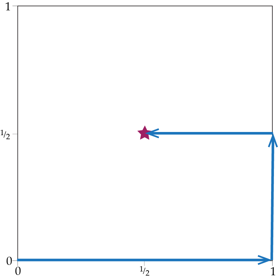
Refer to caption
Figure 6: The path of STON’R for f⁡(θ,ω)=(θ−1/2)⋅(ω−1/2)f(\theta,\omega)=(\theta-1/2)\cdot(\omega-1/2).

First, using our notation in Section 2, let x1x_{1} correspond to θ\theta and x2x_{2} correspond to ω\omega. As explained in the same section, finding a local min-max equilibrium can be reduced to a non-monotone VI problem where V1​(x1,x2):=1/2−x2V_{1}(x_{1},x_{2}):=1/2-x_{2} and V2​(x1,x2):=x1−1/2V_{2}(x_{1},x_{2}):=x_{1}-1/2. Next we describe the steps that our algorithm follows.

  • ⊳\triangleright

    x⁡(0)=(0,0),i=1,S=∅,t=0​, STON’R goes to Step 3.x(0)=(0,0),i=1,S=\emptyset,t=0\text{, STON'R goes to Step 3.} V1​(0,0)=1/2>0V_{1}(0,0)=1/2>0 and x1=0x_{1}=0, hence coordinate 11 is not satisfied. Thus, the loop of Step 22 is activated and STON’R goes to Step 33.

  • ⊳\triangleright

    STON’R goes to Step 55 and executes z˙​(τ)=(1,0)\dot{z}(\tau)=(1,0) with initialization z⁡(0)=(0,0)z(0)=(0,0). Note that at x=(0,0)x=(0,0) the only unit direction satisfying the constraints of Definition 2 is (1,0)(1,0) and that the same is true for any point (⋅,0)(\cdot,0). Thus, for all these points D∅1​((,,,))=(1,0)D^{1}_{\emptyset}((\cdot,0))=(1,0), and the continuous-time dynamics executed at Step 55 is z˙​(τ)=(1,0)\dot{z}(\tau)=(1,0).

  • ⊳\triangleright

    STON’R goes to Step 77 and sets x⁡(1)=(1,0)x(1)=(1,0). For any point z=(z1,0)z=(z_{1},0), V1​(z)=1/2V_{1}(z)=1/2. Thus the continuous-time dynamics of Step 55 only terminates when it hits the boundary of the square at point (1,0)(1,0), which happens at time τexit=1\tau_{\rm exit}=1. At Step 77, the algorithm sets x⁡(1)=z⁡(1)=(1,0)x(1)=z(1)=(1,0).

  • ⊳\triangleright

    STON’R goes to Step 1212 and sets i=2i=2. V1​(x⁡(1))=1/2>0V_{1}(x(1))=1/2>0 thus coordinate 11 is boundary-satisfied at this point. Because this is the good event of Definition 3, the condition of the if statement of Step 88 triggers. Because coordinate 11 is boundary-satisfied the condition of the if statement of Step 99 is not triggered. Thus the algorithm arrives at Step 1212 and sets i=2i=2.

  • ⊳\triangleright

    STON’R goes to Step 33 with i=2i=2, S=∅S=\emptyset. At x⁡(1)=(1,0)x(1)=(1,0) coordinate 11 is boundary-satisfied since V1​(1,0)=1/2>0V_{1}(1,0)=1/2>0 but coordinate 22 is not satisfied since V2​(1,0)=1/2>0V_{2}(1,0)=1/2>0. Thus, the while condition of Step 22 is triggered and STON’R goes to Step 33.

  • ⊳\triangleright

    STON’R goes to Step 55 and executes z˙​(τ)=(0,1)\dot{z}(\tau)=(0,1) with initialization z⁡(0)=(1,0)z(0)=(1,0). Note that at x=(1,0)x=(1,0) the only unit direction satisfying the constraints of Definition 2 is (0,1)(0,1) and that the same is true for any point (1,⋅)(1,\cdot). Thus, for all these points D∅2​((,,,))=(0,1)D^{2}_{\emptyset}((1,\cdot))=(0,1), and the continuous-time dynamics executed at Step 55 is z˙​(τ)=(0,1)\dot{z}(\tau)=(0,1).

  • ⊳\triangleright

    STON’R goes to Step 77 and sets x⁡(1.5)=(1,0.5)x(1.5)=(1,0.5). For any point z=(1,z2)z=(1,z_{2}), V1​(z)=1/2−z2V_{1}(z)=1/2-z_{2} and V2=1/2V_{2}=1/2. Thus the continuous-time dynamics of Step 55 only terminates when it hits point (1,0.5)(1,0.5), which happens at time τexit=1/2\tau_{\rm exit}=1/2. The reason the continuous-time dynamics terminates at this point is because the middling condition of Definition 3 is triggered for j=1j=1. Indeed, coordinate 11 is boundary satisfied from the beginning of the continuous-time dynamics until it reaches point (1,0.5)(1,0.5) but if the continuous-time dynamics were to continue onward, then coordinate 11 would become unsatisfied as V1V_{1} would turn negative. Thus the continuous-time dynamics stops at time τexit=1/2\tau_{\rm exit}=1/2, the algorithm moves to Step 77 and it sets x⁡(1.5)=z⁡(0.5)=(1,0.5)x(1.5)=z(0.5)=(1,0.5).

  • ⊳\triangleright

    STON’R goes to Step 1818 and sets S={1}S=\{1\}. Since the most recently executed continuous-time dynamics at Step 55 ended at a middling exit point, the condition of Step 1717 is activated, so the algorihtm moves to Step 1818 where SS is set to {1}\{1\}.

  • ⊳\triangleright

    STON’R goes to Step 33 with i=2i=2, S={1}S=\{1\}. At x⁡(1.5)=(1,0.5)x(1.5)=(1,0.5) coordinate 11 is both zero- and boundary-satisfied since V1​(1,0.5)=0V_{1}(1,0.5)=0 but coordinate 22 is still not satisfied since V2​(1,0.5)=1/2V_{2}(1,0.5)=1/2. Thus, the while condition of Step 22 is triggered and STON’R goes to Step 33.

  • ⊳\triangleright

    STON’R goes to Step 55 and executes z˙​(τ)=(−1,0)\dot{z}(\tau)=(-1,0) with initialization z⁡(0)=(1,0.5)z(0)=(1,0.5). Note that at x=(1,0.5)x=(1,0.5) the only unit direction satisfying the constraints of Definition 2 is (−1,0)(-1,0) and that the same is true for any point (⋅,0.5)(\cdot,0.5). Thus, for all these points D{1}2​((,,,))=(−1,0)D^{2}_{\{1\}}((\cdot,0.5))=(-1,0), and the continuous-time dynamics executed at Step 55 is z˙​(τ)=(−1,0)\dot{z}(\tau)=(-1,0).

  • ⊳\triangleright

    STON’R goes to Step 77 and sets x⁡(2)=(0.5,0.5)x(2)=(0.5,0.5). For any point z=(z1,0.5)z=(z_{1},0.5), V1​(z)=0V_{1}(z)=0 and V2=z1−1/2V_{2}=z_{1}-1/2. Thus the continuous-time dynamics of Step 55 only terminates when it hits point (0.5,0.5)(0.5,0.5), which happens at time τexit=1/2\tau_{\rm exit}=1/2. The reason the continuous-time dynamics terminates at this point is because the good condition of Definition 3 is triggered for i=2i=2 at this point. Thus the continuous-time dynamics stops at time τexit=1/2\tau_{\rm exit}=1/2, the algorithm moves to Step 77 and it sets x⁡(2)=z⁡(0.5)=(0.5,0.5)x(2)=z(0.5)=(0.5,0.5).

  • ⊳\triangleright

    STON’R goes to Step 2222 and outputs (0.5,0.5)(0.5,0.5). The condition of the if statement of both Steps 88 and 99 are triggered, so S={1,2}S=\{1,2\} and i=3i=3. At x⁡(2)=(0.5,0.5)x(2)=(0.5,0.5) both coordinate 11 and coordinate 22 are satisfied, so the while loop of Step 22 is not activated. So the algorithm goes to Step 2222 and returns (0.5,0.5)(0.5,0.5).

It is easy to verify that the point (θ,ω)=(1/2,1/2)(\theta,\omega)=(1/2,1/2) is a (local) min-max equilibrium of (θ−1/2)⋅(ω−1/2)(\theta-1/2)\cdot(\omega-1/2).

Appendix C Proof of Lemma 1

Proof.

(⟵)(\longleftarrow) Let ZZ denote the zero-satisfied coordinates (Vi​(x)=0V_{i}(x)=0), BS+\mathrm{BS}^{+} the boundary satisfied coordinates with xi=1x_{i}=1 (and thus Vi​(x)>0V_{i}(x)>0) and BS−\mathrm{BS}^{-} the boundary satisfied coordinates with xi=0x_{i}=0 (and thus Vi​(x)<0V_{i}(x)<0). For any y∈[0,1]ny\in[0,1]^{n}, we have ∑i=1nVi​(x)​(xi−yi)≥0\sum_{i=1}^{n}V_{i}(x)(x_{i}-y_{i})\geq 0, which can easily be seen by breaking up the sum into three sums corresponding to indices in ZZ, BS+\mathrm{BS}^{+} and BS−\mathrm{BS}^{-}.

(⟶)(\longrightarrow) Let x∈[0,1]nx\in[0,1]^{n} be a solution of the V, i.e. V​(x)⊤​(x−y)≤0V(x)^{\top}(x-y)\leq 0 for all y∈[0,1]ny\in[0,1]^{n}. Consider an arbitrary i∈[n]i\in[n] and a vector yy such that yj=xjy_{j}=x_{j} for all j≠ij\neq i. If xi=1x_{i}=1, take yi=0y_{i}=0, and plug this into V​(x)​(x−y)≤0V(x)(x-y)\leq 0 to get Vi​(x)≥0V_{i}(x)\geq 0. If xi=0x_{i}=0, take yi=1y_{i}=1, and plug this into V​(x)⊤​(x−y)≤0V(x)^{\top}(x-y)\leq 0 to get Vi​(x)≤0V_{i}(x)\leq 0. If xi∈(0,1)x_{i}\in(0,1) consider first yi=xi+δy_{i}=x_{i}+\delta for some small δ>0\delta>0 and plug this into V​(x)⊤​(x−y)≤0V(x)^{\top}(x-y)\leq 0 we get V⁡(xi)≥0V(x_{i})\geq 0. By repeating the same argument for yi=xi−δy_{i}=x_{i}-\delta we that get Vi​(x)≤0V_{i}(x)\leq 0. As a result, Vi​(x)=0V_{i}(x)=0. ∎

Appendix D Proof of Theorem 1

In this section we present the proof of Theorem 1. The proof follows closely the sketch exhibited in Section 5.3 with some slight modifications on the definition of the nodes NN of the directed graph GG.

D.1 Helpful Definitions and Lemmas

We start with the definition of pivots that will play the role of nodes NN.

Definition 4.

A point x∈[0,1]nx\in[0,1]^{n} is called a pivot if and only if the following hold,

  • •

    If coordinate ii is not satisfied then Vi​(x)>0V_{i}(x)>0.

  • •

    If ℓ\ell is the minimum unsatisfied coordinate then xj=0x_{j}=0 for all coordinates j≥ℓ+1j\geq\ell+1.

  • •

    If ℓ\ell is the minimum unsatisfied coordinate then there exists at least one coordinate j∈M∪{ℓ}j\in M\cup\{\ell\} with xj=0x_{j}=0 or xj=1x_{j}=1 where M:={j≤ℓ−1:Vj​(x)=0}M:=\{j\leq\ell-1:\penalty\ V_{j}(x)=0\}.

As in the proof sketch of Section 5.3, given a pivot xx (that admits at least one unsatisfied variable) we argue that STOR’N visits another pivot at some finite time. As depicted in Dynamics 2, the latter happens by following the continuous curve z˙​(t)=DSi​(z⁡(t))\dot{z}(t)=D_{S}^{i}(z(t)). Recall that in Dynamics 2 the pair (i,S)(i,S) is updated in the previous steps of the algorithm (Steps 8,13,158,13,15 and 1717). In the next Definitions 5, 6 and 7, we provide an alternative way of "computing locally" the pair (i,S)(i,S) by using only the knowledge of x⁡(t)x(t) at Step 33 of Dynamics 2.

Definition 5.

Consider the direction DSi​(x):=(d1,…,dn)D^{i}_{S}(x):=(d_{1},\ldots,d_{n}) of Definition 2 for the set of zero-satisfied coordinates S={j<i with Vj(x)=0}S=\{j<i\text{ with }V_{j}(x)=0\} (recall that dj=0d_{j}=0 for all j∉S∪{i}j\notin S\cup\{i\}). If, for all k∈Sk\in S, one of the following holds: (a) xk∈(0,1)x_{k}\in(0,1), or (b) xk=0x_{k}=0 and dk≥0d_{k}\geq 0, or (c) xk=1x_{k}=1 and dk≤0d_{k}\leq 0, then we define Di​(x):=DSi​(x)D^{i}(x):=D_{S}^{i}(x). Otherwise, let j∈Sj\in S be the unique coordinate (uniqueness follows from Assumption 2) such that either {xj=0\{x_{j}=0 and dj<0}d_{j}<0\} or {xj=1\{x_{j}=1 and dj>0}d_{j}>0\}, and we define Di​(x):=DS∖{j}i​(x)D^{i}(x):=D_{S\setminus\{j\}}^{i}(x). Di​(x)D^{i}(x) is called the ideal direction of movement at point x∈[0,1]nx\in[0,1]^{n} with respect to coordinate ii.

Definition 6.

Given a point x∈[0,1]nx\in[0,1]^{n} coordinate ii is called frozen if and only if (xi=0x_{i}=0 and 𝑂𝑃𝐸𝑁[Di​(x)]i<0)[D^{i}(x)]_{i}<0) or (xi=1x_{i}=1 and 𝑂𝑃𝐸𝑁[Di​(x)]i>0)[D^{i}(x)]_{i}>0) where Di​(x)D^{i}(x) is the ideal direction at xx with respect to coordinate ii (Definition 5).

Definition 7.

Given a pivot x∈[0,1]nx\in[0,1]^{n} consider

  • •

    ℓ:=min1≤j≤n⁡{coordinate ​j​ is not satisfied at ​x}.\ell:=\min_{1\leq j\leq n}\{\text{coordinate }j\text{ is not satisfied at }x\}.

  • •

    i:=maxj≤ℓ⁡{coordinate ​j​ is not frozen at ​x}i:=\max_{j\leq\ell}\{\text{coordinate }j\text{ is not frozen at }x\}.

  • •

    S←S\leftarrow the set of coordinates such that Di​(⋅)=DSi​(⋅)D^{i}(\cdot)=D_{S}^{i}(\cdot) (see Definition 5).

The coordinate ii is called the under examination coordinate, the pair (i,S)(i,S) is called the admissible pair for pivot xx.

Remark 2.

Computing the (i,S)(i,S) admissible pair of the pivot x⁡(t)x(t) at Step 33 in Dynamics 2 is equivalent with Dynamics 2 at which (i,S)(i,S) is updated at Steps 8,13,158,13,15 and 1717.

D.2 Main Steps of the Proof

To simplify notation we describe STOR’N using the notion of pivots and admissible pairs (i,S)(i,S) of Definition 4 and 7.

Dynamics 3 STay-ON-the-Ridge (STON’R)
1:  Initially x⁡(0)←(0,…,0)x{(0)}\leftarrow(0,\ldots,0), i←1i\leftarrow 1, S←∅S\leftarrow\emptyset, t←0t\leftarrow 0.
2:  while x⁡(t)x{(t)} is not a VI solution do
3:   At point x⁡(t)x(t) compute the admissible pair (i,S)(i,S) for pivot x⁡(t)x(t).
4:   Follows the continuous-time dynamics, z˙​(τ)=DSi​(z⁡(τ))\dot{z}(\tau)=D^{i}_{S}(z(\tau)), at z⁡(0)=x⁡(t)z(0)=x{(t)}.
5:   while z⁡(τ){z}(\tau) is not an exit point as per Definition 3 do
6:    Execute z˙​(τ)=DSi​(z⁡(τ))\dot{z}(\tau)=D^{i}_{S}(z(\tau)) forward in time.
7:   end while
8:   Set x⁡(t+τ)=z⁡(τ)x{(t+\tau)}=z(\tau) for all τ∈[0,τexit]\tau\in[0,\tau_{\rm exit}] (where τexit\tau_{\rm exit} is earliest time z⁡(τ){z}(\tau) became an exit point).
9:   Set t←t+τexitt\leftarrow t+\tau_{\rm exit}.
10:  end while
11:  return x⁡(t)x(t)

We are now ready to present the topological argument described in Section 5.3. As already mentioned the nodes NN of the directed graph GG will be the set of pivots while we say that there exists an edge (x,x′)(x,x^{\prime}) from pivot xx to pivot x′x^{\prime} in case setting z⁡(0):=xz(0):=x and following the direction z˙​(t)=DSi​(z⁡(t))\dot{z}(t)=D_{S}^{i}(z(t)) (where (i,S)(i,S) is the admissible pair of xx) leads to pivot x′x^{\prime} once one of the "if" loops in Steps 9,11,139,11,13 and 1515 is activated.

In Lemma 3 we establish the fact that the pivots which correspond to the number of nodes of directed graph GG are finite.

Lemma 3.

There exists a finite number of pivots.

In Definition 8 we formalize the notion of directed edge (x,x′)(x,x^{\prime}) in graph GG which we additionally denote as x′=Next⁡(x)x^{\prime}=\mathrm{Next}(x).

Definition 8.

Given a pivot x∈[0,1]nx\in[0,1]^{n} consider the trajectory z˙​(t)=DSi​(z⁡(t))\dot{z}(t)=D_{S}^{i}(z(t)) with z⁡(0)=xz(0)=x where (i,S)(i,S) is the admissible pair of xx. We say that pivot x′x^{\prime} is the next pivot of xx, i.e. x′=Next⁡(x)x^{\prime}=\mathrm{Next}(x) if and only if there exists t∗>0t^{\ast}>0 such that

  • •

    z⁡(t∗)=x′z(t^{\ast})=x^{\prime}

  • •

    z⁡(t)z(t) is not a pivot for all t∈(0,t∗)t\in(0,t^{\ast}).

In Lemma 4 we establish the fact that any pivot with at least one unsatisfied variable must necessarily admit outdegree equal to 11. The latter directly implies that any pivot with outdegree 00 must correspond to a solution since all coordinates are satisfied.

Lemma 4.

For any pivot x∈[0,1]nx\in[0,1]^{n} with at least one unsatisfied coordinate there exists a pivot x′x^{\prime} such that x′=Next⁡(x)x^{\prime}=\mathrm{Next}(x). Moreover let (i,S)(i,S) be the admissible pair for pivot xx, z⁡(t)z(t) be the trajectory z˙​(t)=DSi​(z⁡(t))\dot{z}(t)=D_{S}^{i}(z(t)) with z⁡(0)=xz(0)=x and t′t^{\prime} be the time at which x′=z⁡(t′)x^{\prime}=z(t^{\prime}). Then for all t∈[0,t′]t\in[0,t^{\prime}],

  • •

    all coordinates j∈Sj\in S admit Vj​(z​(t))=0V_{j}(z(t))=0.

  • •

    all coordinates j≤i−1j\leq i-1 are satisfied at z⁡(t)z(t).

  • •

    all coordinates j≥i+1j\geq i+1 admit zj​(t)=0z_{j}(t)=0.

  • •

    all coordinates jj admit zj​(t)∈[0,1]z_{j}(t)\in[0,1].

Using Lemma 4 we additionally obtain Corollary 1 ensuring that the point x⁡(t)x(t) at Step 33 of Dynamics 3 is always a pivot and thus Dynamics 3 is well-defined.

Corollary 1.

Let x⁡(t)x(t) at Step 33 of Dynamics 3 be a pivot. Then the point x⁡(t+τe​x​i​t)x(t+\tau_{exit}) at Step 88 of Dynamics 3 is also a pivot. Moreover the point (0,…,0)(0,\ldots,0) is a pivot.

In Lemma 5 we establish the fact that no pivot/node can admit in-degree more than 22. The latter implies if we start with a pivot with 00 in-degree we must essentially visit a pivot with out-degree 00 that consists a solution.

Lemma 5.

Any pivot x∈[0,1]nx\in[0,1]^{n} admits in-degree at most 11. In other words in case x∗=Next⁡(x1)x^{\ast}=\mathrm{Next}(x_{1}) and x∗=Next⁡(x2)x^{\ast}=\mathrm{Next}(x_{2}) for some pivots x1,x2x_{1},x_{2} then x1=x2x_{1}=x_{2}.

We conclude the proof by showing that (0,…,0)(0,\ldots,0) that is the initial pivot that Dynamics 3 visits admits 00 in-degree.

Lemma 6.

There is no pivot x∈[0,1]nx\in[0,1]^{n} such that Next⁡(x)=(0,…,0)\mathrm{Next}(x)=(0,\ldots,0).

Appendix E Proof of Lemma 3

Lemma 7.

Let the functions F1​(x),…,Fi​(x)F_{1}(x),\ldots,F_{i}(x) where Fℓ:[0,1]i↦ℝF_{\ell}:[0,1]^{i}\mapsto\mathbb{R} and the set B:={x∈[0,1]i:Fℓ(x)=0for all ℓ=1,…,i}B:=\{x\in[0,1]^{i}:\penalty\ \penalty\ F_{\ell}(x)=0\penalty\ \penalty\ \text{for all }\ell=1,\ldots,i\}. In case F1,…,FℓF_{1},\ldots,F_{\ell} satisfy the following assumptions

  • •

    ∥∇Fℓ​(x)−∇Fℓ​(y)∥2≤L⋅∥x−y∥2\lVert\nabla F_{\ell}(x)-\nabla F_{\ell}(y)\rVert_{2}\leq L\cdot\lVert x-y\rVert_{2}

  • •

    For all x∈Bx\in B the matrix

    J⁡(x):=(∂F1​(x)∂x1…∂F1​(x)∂xi∂Fi​(x)∂x1…∂Fi​(x)∂xi)J(x):=\begin{pmatrix}\frac{\partial F_{1}(x)}{\partial x_{1}}&\ldots&\frac{\partial F_{1}(x)}{\partial x_{i}}\\ \vdots&&\vdots\\ \frac{\partial F_{i}(x)}{\partial x_{1}}&\ldots&\frac{\partial F_{i}(x)}{\partial x_{i}}\end{pmatrix}

    admits singular values that are at least σmin\sigma_{\text{min}} and at most σmax\sigma_{\text{max}}.

Then the set BB is finite. More precisely, |B|≤2i/Voli​(2​σm​i​n2i​L​σm​a​x2)|B|\leq 2^{i}/\text{Vol}^{i}\left(\frac{2\sigma^{2}_{min}}{\sqrt{i}L\sigma^{2}_{max}}\right) where Voli​(ρ)\text{Vol}^{i}(\rho) is the volume of the ii-dimensional ball with radius ρ\rho.

Lemma 3 directly follows by Lemma 7. More precisely, we get that the number of pivots in [0,1]n[0,1]^{n} is at most n⋅4n/Voln​(2​σm​i​n2n​L​σm​a​x2)n\cdot 4^{n}/\text{Vol}^{n}\left(\frac{2\sigma^{2}_{min}}{\sqrt{n}L\sigma^{2}_{max}}\right).

E.1 Proof of Lemma 7

Let us assume the existence of x,y∈Bx,y\in B such that ∥x−y∥2≤ρ\lVert x-y\rVert_{2}\leq\rho and x≠yx\neq y. Notice that the ∇F1​(x),…,∇Fi​(x)\nabla F_{1}(x),\ldots,\nabla F_{i}(x) are linearly independent and thus

x−y=∑j=1iμj⋅∇Fj​(x)x-y=\sum_{j=1}^{i}\mu_{j}\cdot\nabla F_{j}(x)

which implies that

∥μ∥2≤ρσmin\lVert\mu\rVert_{2}\leq\frac{\rho}{\sigma_{\text{min}}} (5)

By Taylor expansion of xx and the fact that ∥∇Fℓ​(x)−∇Fℓ​(y)∥≤L⋅∥x−y∥2\lVert\nabla F_{\ell}(x)-\nabla F_{\ell}(y)\rVert\leq L\cdot\lVert x-y\rVert_{2} we get,

|Fℓ​(y)−Fℓ​(x)−(∇Fℓ​(x))⊤⋅∑j=1iμj⋅∇Fj​(x)|≤12​L⋅∥∑ℓ=1iμj⋅∇Fj​(x)∥2\left|F_{\ell}(y)-F_{\ell}(x)-(\nabla F_{\ell}(x))^{\top}\cdot\sum_{j=1}^{i}\mu_{j}\cdot\nabla F_{j}(x)\right|\leq\frac{1}{2}L\cdot\lVert\sum_{\ell=1}^{i}\mu_{j}\cdot\nabla F_{j}(x)\rVert^{2}

which due to the fact that Fℓ​(y)=Fℓ​(x)=0F_{\ell}(y)=F_{\ell}(x)=0 implies,

[J⊤​(x)⋅J⁡(x)⋅μ]ℓ≤12​L⋅σmax2⋅∥μ∥2\left[J^{\top}(x)\cdot J(x)\cdot\mu\right]_{\ell}\leq\frac{1}{2}L\cdot\sigma^{2}_{\text{max}}\cdot\lVert\mu\rVert^{2}

and thus

∥μ∥2≥2​σmini​L​σmax2\lVert\mu\rVert_{2}\geq\frac{2\sigma_{\text{min}}}{\sqrt{i}L\sigma^{2}_{\text{max}}} (6)

Combining Equation 5 and 6 we get ρ≥2​σmin2i​L​σmax2\rho\geq\frac{2\sigma^{2}_{\text{min}}}{\sqrt{i}L\sigma^{2}_{\text{max}}}. To this end we know that in case x,y∈Bx,y\in B with x≠yx\neq y then ∥x−y∥2≥2​σmin2i​L​σmax2\lVert x-y\rVert_{2}\geq\frac{2\sigma^{2}_{\text{min}}}{\sqrt{i}L\sigma^{2}_{\text{max}}}. Thus,

|B|≤2i/Voli​(2​σm​i​n2i​L​σm​a​x2)|B|\leq 2^{i}/\text{Vol}^{i}\left(\frac{2\sigma^{2}_{min}}{\sqrt{i}L\sigma^{2}_{max}}\right)

Appendix F Proof of Lemma 4

Lemma 8.

Let a pivot x∈[0,1]nx\in[0,1]^{n} and (i,S)(i,S) the admissible pair for xx. Then the following hold,

  • •

    There exists a unique trajectory z⁡(t)z(t) with z˙​(t)=DSi​(z⁡(t))\dot{z}(t)=D^{i}_{S}\left(z(t)\right) and z⁡(0)=xz(0)=x.

  • •

    Vj​(z​(t))=0V_{j}(z(t))=0 for all coordinates j∈Sj\in S.

  • •

    There exists t∗>0t^{\ast}>0 such that for all t∈[0,t∗]t\in[0,t^{\ast}] all coordinates j≤i−1j\leq i-1 are satisfied at z⁡(t)z(t) and zj​(t)∈[0,1]z_{j}(t)\in[0,1] for all coordinates jj.

Lemma 9.

Let a set of coordinates SS, a coordinate ii and a point x∈[0,1]x\in[0,1] such that xj∈(0,1)x_{j}\in(0,1) for all j∈S∪{i}j\in S\cup\{i\}. Consider the trajectory γ˙​(t)=DSi​(γ⁡(t))\dot{\gamma}(t)=D_{S}^{i}(\gamma(t)) with γ⁡(0)=x\gamma(0)=x. Then there exists t∗∈(0,C]t^{\ast}\in(0,C] such that

γj​(t∗)=0​ or ​1 for some ​j∈S∪{i}\gamma_{j}(t^{\ast})=0\text{ or }1\penalty\ \penalty\ \text{ for some }j\in S\cup\{i\}

where CC is constant depending on the parameters σmin,σmax\sigma_{\text{min}},\sigma_{\text{max}} and LL.

Lemma 10.

Let a pivot x∈[0,1]nx\in[0,1]^{n} with at least one unsatisfied coordinate. Let (i,S)(i,S) the admissible pair of pivot xx (Definition 7) and ℓ\ell the minimum unsatisfied coordinate at xx. Then the following hold,

  • •

    The under examination variable admits i≥1i\geq 1.

  • •

    xj=0​ for all coordinates ​j≥i+1.x_{j}=0\text{ for all coordinates }j\geq i+1.

Additionally one of the following holds,

  • •

    i=ℓi=\ell and Vℓ​(x)>0V_{\ell}(x)>0

  • •

    xi=1x_{i}=1 and Vi​(x)>0V_{i}(x)>0

  • •

    Vi​(x)=0V_{i}(x)=0 and DSi(x)⊤∇Vi(x)>0D_{S}^{i}(x)^{\top}\nabla V_{i}(x)>0

F.1 Proof of Lemma 4

Given the pivot x∈[0,1]nx\in[0,1]^{n} with at least one unsatisfied variable and let (i,S)(i,S) denote its admissible pair. By Lemma 10 we know that the under examination variable ii admits i≥1i\geq 1. Now consider the the trajectory z˙​(t)=DSi​(z⁡(t))\dot{z}(t)=D^{i}_{S}(z(t)) with z⁡(0)=xz(0)=x. Due to the fact that i≥1i\geq 1 and by Assumption 3 we known that for all t∈(0,δ)t\in(0,\delta) where δ>0\delta>0 is sufficiently small, the following hold

  • •

    zj​(t)∈(0,1)z_{j}(t)\in(0,1) for all j∈S∪{i}j\in S\cup\{i\}

  • •

    zj​(t)=0z_{j}(t)=0 or zj​(t)=1z_{j}(t)=1 for all coordinates j∉S∪{i}j\notin S\cup\{i\}.

By Lemma 9 there exists t∗>0t^{\ast}>0 such that zj​(t∗)=0z_{j}(t^{\ast})=0 or 11 for some coordinate j∈S∪{i}j\in S\cup\{i\} and OPENzj​(t)∈[0,1])z_{j}(t)\in[0,1]) for all coordinates jj and t∈[0,t∗]t\in[0,t^{\ast}].

We first show that if there exists a coordinate j≤i−1j\leq i-1 such that jj is not satisfied at z⁡(t∗)z(t^{\ast}) then there exists t^<t∗\hat{t}<t^{\ast} such that z⁡(t^)z(\hat{t}) is a pivot.

Let ℓ\ell denote the unsatisfied coordinate at z⁡(t∗)z(t^{\ast}). Notice that by Lemma 8 all coordinates j∈Sj\in S admit Vj​(z⁡(t∗))=0V_{j}\left(z(t^{\ast})\right)=0 and thus ℓ∉S\ell\notin S. The latter implies that (xℓ=0x_{\ell}=0 and Vℓ​(x)≤0V_{\ell}(x)\leq 0) or (xℓ=1x_{\ell}=1 and Vℓ​(x)≥0V_{\ell}(x)\geq 0) and since coordinate ℓ\ell stands still in the trajectory z˙​(t)=DSi​(z⁡(t))\dot{z}(t)=D_{S}^{i}(z(t)), zℓ​(t^)=xℓz_{\ell}(\hat{t})=x_{\ell} there are two mutually exclusives cases:

  • •

    xℓ=zℓ​(t^)=0x_{\ell}=z_{\ell}(\hat{t})=0, Vℓ​(x)≤0V_{\ell}(x)\leq 0 and Vℓ​(z​(t^))>0V_{\ell}(z(\hat{t}))>0

  • •

    xℓ=zℓ​(t^)=1x_{\ell}=z_{\ell}(\hat{t})=1, Vℓ​(x)≥0V_{\ell}(x)\geq 0 and Vℓ​(z​(t^))<0V_{\ell}(z(\hat{t}))<0

Then by Lemma 12 we additionally get that for sufficiently small δ>0\delta>0,

  • •

    If xℓ=0x_{\ell}=0 then Vℓ​(z​(t))<0V_{\ell}(z(t))<0 for t∈(0,δ)t\in(0,\delta)

  • •

    If xℓ=1x_{\ell}=1 then Vℓ​(z​(t))>0V_{\ell}(z(t))>0 for t∈(0,δ)t\in(0,\delta)

As a result, in any case there exists tℓ∈(0,t∗)t_{\ell}\in(0,t^{\ast}) such that Vℓ​(z⁡(tℓ))=0V_{\ell}(z(t_{\ell}))=0, coordinate ℓ\ell lies on the boundary at z⁡(tℓ)=0z(t_{\ell})=0 and coordinate ℓ\ell is satisfied at z⁡(t)z(t) for all t∈[0,tℓ]t\in[0,t_{\ell}].

Now consider the set of coordinates A:={j≤i−1:coordinate ​j​ is not satisfied at ​z​(t∗)}A:=\{j\leq i-1:\penalty\ \text{coordinate }j\text{ is not satisfied at }z(t^{\ast})\} and let t^:=minℓ∈A⁡t^ℓ\hat{t}:=\min_{\ell\in A}\hat{t}_{\ell}. Then all coordinates j≤i−1j\leq i-1 are satisfied at z⁡(t^)z(\hat{t}) while there exists a coordinate ℓ^∈A\hat{\ell}\in A such that Vℓ^​(z​(t^))=0V_{\hat{\ell}}(z(\hat{t}))=0 with coordinate ℓ^\hat{\ell} being on the boundary at z⁡(t^)z(\hat{t}). Up next we argue that z⁡(t^)z(\hat{t}) is a pivot.

Consider the set of coordinates M:={j≤i−1:Vj​(z⁡(t^))=0}M:=\{j\leq i-1:\penalty\ V_{j}(z(\hat{t}))=0\}. Since ℓ^∈M\hat{\ell}\in M and ℓ^\hat{\ell} lies on the boundary at z⁡(t^)z(\hat{t}) the third item of Definition 4 is satisfied. Since xx is a pivot, Lemma 10 implies all coordinates j≥i+1j\geq i+1 admit xj=0x_{j}=0. Since [DSi​(⋅)]j=0[D^{i}_{S}(\cdot)]_{j}=0 for all j≥i+1j\geq i+1 the latter implies that zj​(t^)=xj=0z_{j}(\hat{t})=x_{j}=0. Due to the fact that all coordinates j≤i−1j\leq i-1 are satisfied at z⁡(t^)z(\hat{t}) we get that the second item of Definition 4 is satisfied. Finally notice that by Lemma 10, Vi​(z​(t))>0V_{i}(z(t))>0 for all t∈(0,δ)t\in(0,\delta) for sufficiently small δ\delta. In case Vi​(z​(t^))<0V_{i}(z(\hat{t}))<0 then there exist t′<t^t^{\prime}<\hat{t} such that V⁡(z⁡(t′))=0V(z(t^{\prime}))=0 implying that z⁡(t′)z(t^{\prime}) is a pivot. As a result, without loss of generality we assume that Vi​(z​(t^))>0V_{i}(z(\hat{t}))>0 which implies that the first item of Definition 4 is satisfied.

As a result, without loss of generality we assume that all coordinates j≤i−1j\leq i-1 are satisfied for all z⁡(t)z(t) in [0,t∗][0,t^{\ast}]. Up next we show that in this case either the point x∗:=z⁡(t∗)x^{\ast}:=z(t^{\ast}) is a pivot or z⁡(t^)z(\hat{t}) is pivot for some t^∈(0,t∗)\hat{t}\in(0,t^{\ast}).

Notice that by Lemma 10 all coordinates j≥i+1j\geq i+1 admit xj=0x_{j}=0. Since [DSi​(⋅)]j=0[D^{i}_{S}(\cdot)]_{j}=0 for all j≥i+1j\geq i+1 the latter implies that xj∗=xj=0x_{j}^{\ast}=x_{j}=0. As a result, xj∗=0x_{j}^{\ast}=0 for all j≥i+1j\geq i+1. Due to our assumption that all coordinates j≤i−1j\leq i-1 are satisfied at x∗x^{\ast}, the minimum unsatisfied coordinate at x∗x^{\ast} is greater than ii and thus the second item of Definition 4 is satisfied. Moreover due to the fact that xj∗=0x_{j}^{\ast}=0 or 11 for some j∈S∪{i}j\in S\cup\{i\} and Vj​(x∗)=0V_{j}(x^{\ast})=0 for all j∈Sj\in S, the third item of Definition 4 is satisfied.

Up next we argue that in case coordinate ii is not satisfied at x∗x^{\ast} then Vi​(x∗)>0V_{i}(x^{\ast})>0. Let us assume that coordinate ii is not satisfied at x∗x^{\ast} and Vi​(x∗)<0V_{i}(x^{\ast})<0. Let ℓ\ell denote the minimum unsatisfied variable at xx then Lemma 10 provides us with the following mutually exclusive cases:

  • •

    i=ℓi=\ell then Vℓ​(x)>0V_{\ell}(x)>0: Since Vℓ​(z⁡(0))=Vℓ​(z)>0V_{\ell}(z(0))=V_{\ell}(z)>0 and Vℓ​(z⁡(t∗))=Vℓ​(x∗)<0V_{\ell}(z(t^{\ast}))=V_{\ell}(x^{\ast})<0 there exists t^∈(0,t∗)\hat{t}\in(0,t^{\ast}) such that Vℓ​(z​(t^))=0V_{\ell}(z(\hat{t}))=0. Notice that z⁡(t^)z(\hat{t}) satisfies all the three items of Definition 4.

  • •

    xi=1x_{i}=1 with Vi​(x)>0V^{i}(x)>0: Same as above.

  • •

    Vi​(x)=0V_{i}(x)=0 and DSi​(x)⊤⋅Vi​(x)>0D_{S}^{i}(x)^{\top}\cdot V^{i}(x)>0: Notice that Vi​(z​(t))>0V_{i}(z(t))>0 for all t∈(0,δ)t\in(0,\delta) once δ\delta is selected sufficiently small. By repeating the same argument as above we conclude that there is t^\hat{t} such that z⁡(t^)z(\hat{t}) is a pivot.

F.2 Proof of Lemma 8

Let the set of coordinates SS, we first establish in Lemma 11 that DSi​(x)D^{i}_{S}(x) is MM-Lipschitz. The proof of Lemma 11 is presented at Section F.4

Lemma 11.

Let x∈[0,1]nx\in[0,1]^{n} and a set of coordinates SS such that Vj​(x)=0V_{j}(x)=0 for all j∈Sj\in S. Then for any coordinate i∉Si\notin S and for any y∈ℝny\in\mathbb{R}^{n} such that ∥x−y∥2≤σmin/2​L​n\lVert x-y\rVert_{2}\leq\sigma_{\text{min}}/2L\sqrt{n},

∥DSi​(x)−DSi​(y)∥2≤M⋅∥x−y∥2\lVert D^{i}_{S}(x)-D^{i}_{S}(y)\rVert_{2}\leq M\cdot\lVert x-y\rVert_{2}

for M:=Θ⁡(σmaxσmin2⋅n⋅L)M:=\Theta\left(\frac{\sigma_{\text{max}}}{\sigma^{2}_{\text{min}}}\cdot\sqrt{n}\cdot L\right).

To simplify notation let Zi(x):={ℓ<i such that Vℓ(x)=0}Z^{i}(x):=\{\ell<i\text{ such that }V_{\ell}(x)=0\} and Fi(x):={ℓ<i such that coordinate ℓ is fixed at x}F^{i}(x):=\{\ell<i\text{ such that coordinate }\ell\text{ is fixed at }x\}. Since xx is a pivot, all coordinates ℓ≤i−1\ell\leq i-1 are satisfied and thus each coordinate ℓ≤i−1\ell\leq i-1 either belongs to Zi​(x)Z^{i}(x) or to Fi​(x)F^{i}(x).

Let us first consider the case where one of the following holds for all coordinates ℓ∈Zi​(x)\ell\in Z^{i}(x).

  • •

    xℓ∈(0,1)x_{\ell}\in(0,1)

  • •

    xℓ=0x_{\ell}=0 and [DZi​(x)i]ℓ≥0[D^{i}_{Z_{i}(x)}]_{\ell}\geq 0

  • •

    xℓ=1x_{\ell}=1 and [DZi​(x)i]ℓ≤0[D^{i}_{Z_{i}(x)}]_{\ell}\leq 0

Notice that in this case Definition 5 and 7 imply S=Zi​(x)S=Z^{i}(x). Now consider the set B:={y∈ℝn such that ∥x−y∥2≤σmin/2L}B:=\{y\in\mathbb{R}^{n}\text{ such that }\lVert x-y\rVert_{2}\leq\sigma_{\min}/2L\}. Then combining Lemma 11 with the Picard–Lindelöf theorem we get that there exists a unique z⁡(t)z(t) such that

  1. 1.

    z˙​(t)=DSi​(z⁡(t))\dot{z}(t)=D^{i}_{S}\left(z(t)\right)

  2. 2.

    z⁡(0)=xz(0)=x

By taking δ>0\delta>0 sufficiently small we get that for all t∈[0,δ]t\in[0,\delta] the following hold,

  • •

    Vℓ​(z​(t))=0V_{\ell}\left(z(t)\right)=0 for all ℓ∈S\ell\in S

  • •

    zℓ​(t)∈(0,1)z_{\ell}(t)\in(0,1) for all ℓ∈S\ell\in S.

  • •

    coordinate ℓ\ell is boundary satisfied at z⁡(t)z(t) for all ℓ∈{1,…,i−1}/S\ell\in\{1,\ldots,i-1\}/S.

  • •

    zj​(t)∈[0,1]nz_{j}(t)\in[0,1]^{n} for all coordinates jj.

Now consider the case in which there exists a coordinate j∈Zi​(x)j\in Z^{i}(x) such that (xj=0x_{j}=0 and [DZi​(x)i]j<0[D^{i}_{Z_{i}(x)}]_{j}<0) or (xj=1x_{j}=1 and [DZi​(x)i]j>0[D^{i}_{Z_{i}(x)}]_{j}>0). By Assumption 2 we know that such a coordinate must be unique. In this case by Definition 5 we get Di​(x)=DZi​(x)/{j}i​(x)D^{i}(x)=D^{i}_{Z^{i}(x)/\{j\}}(x) and thus by Definition 7, S=Zi​(x)/{j}S=Z^{i}(x)/\{j\}.

Lemma 12 establish the fact that in this case following the direction DSi​(x)D^{i}_{S}(x) consists the variable jj boundary satisfied. The proof of Lemma 12 is presented in Section F.3.

Lemma 12.

For any x∈[0,1]nx\in[0,1]^{n} if there exists coordinate jj with

  • •

    xj=0x_{j}=0 and [DZi​(x)i​(x)]j<0[D^{i}_{Z^{i}(x)}(x)]_{j}<0 then (DZi​(x)/{j}i​(x))⊤⋅∇Vj​(x)<0\left(D^{i}_{Z^{i}(x)/\{j\}}(x)\right)^{\top}\cdot\nabla V_{j}(x)<0.

  • •

    xj=1x_{j}=1 and [DZi​(x)i​(x)]j>0[D^{i}_{Z^{i}(x)}(x)]_{j}>0 then (DZi​(x)/{j}i​(x))⊤⋅∇Vj​(x)>0\left(D^{i}_{Z^{i}(x)/\{j\}}(x)\right)^{\top}\cdot\nabla V_{j}(x)>0.

By the exact same arguments as above, we get that there exists a unique trajectory z⁡(t)z(t) such that z˙​(t)=DSi​(z⁡(t))\dot{z}(t)=D^{i}_{S}\left(z(t)\right) and x⁡(0)=xx(0)=x and by taking δ>0\delta>0 sufficiently small we get,

  • •

    Vℓ​(z​(t))=0V_{\ell}\left(z(t)\right)=0 for all ℓ∈S\ell\in S

  • •

    zℓ​(t)∈(0,1)z_{\ell}(t)\in(0,1) for all ℓ∈S\ell\in S

  • •

    coordinate ℓ\ell is boundary satisfied at z⁡(t)z(t) for all ℓ∈Fi​(x)\ell\in F^{i}(x)

  • •

    zj​(t)∈[0,1]nz_{j}(t)\in[0,1]^{n} for all coordinates jj.

In order to complete the proof of Lemma 8 we need to argue that the coordinate jj is satisfied for all z⁡(t)z(t) with t∈[0,δ′]t\in[0,\delta^{\prime}]. Without loss of generality consider xj=0x_{j}=0 (the case xj=1x_{j}=1 follows symmetrically). Recall that Vj​(x)=0V_{j}(x)=0 and by Lemma 12 we get that (DSi​(x))⊤⋅∇Vj​(x)<0\left(D_{S}^{i}(x)\right)^{\top}\cdot\nabla V_{j}(x)<0. Thus by selecting δ′<δ\delta^{\prime}<\delta sufficiently small we get

Vj​(z⁡(t))<0 and zj​(t)=0V_{j}\left(z(t)\right)<0\penalty\ \penalty\ \text{ and }\penalty\ \penalty\ z_{j}(t)=0

for all t∈(0,δ′]t\in(0,\delta^{\prime}].

F.3 Proof of Lemma 12

To simplify notation let Zi​(x)={1,…,i−1}Z^{i}(x)=\{1,\ldots,i-1\}, DZi​(x)i​(x)=(d1,…,dj,…,di)D^{i}_{Z^{i}(x)}(x)=(d_{1},\ldots,d_{j},\ldots,d_{i}) and DZi​(x)/{j}i​(x)=(d^1,…,d^j−1,d^j−1,…,d^i)D^{i}_{Z^{i}(x)/\{j\}}(x)=(\hat{d}_{1},\ldots,\hat{d}_{j-1},\hat{d}_{j-1},\ldots,\hat{d}_{i}). Moreover let assume that xj=0x_{j}=0 and ii is even. The cases xj=0x_{j}=0 and ii is odd, xj=1x_{j}=1 and ii is even, xj=1x_{j}=1 and ii is odd follow symmetrically.

We will prove that

(d1^,…,d^j−1,d^j+1,…,d^i)⊤⋅(∂Vj​(x)∂x1,…,∂Vj​(x)∂xj−1,∂Vj​(x)∂xj+1,…,∂Vj​(x)∂xi−1)<0\left(\hat{d_{1}},\ldots,\hat{d}_{j-1},\hat{d}_{j+1},\ldots,\hat{d}_{i}\right)^{\top}\cdot\left(\frac{\partial V_{j}(x)}{\partial x_{1}},\ldots,\frac{\partial V_{j}(x)}{\partial x_{j-1}},\frac{\partial V_{j}(x)}{\partial x_{j+1}},\ldots,\frac{\partial V_{j}(x)}{\partial x_{i-1}}\right)<0

Since ii is even we get by Definition 2,

|∂V1​(x)∂x1…∂Vj−1​(x)∂x1∂Vj+1​(x)∂x1…∂Vi−1​(x)∂x1d^1∂V1​(x)∂xj−1…∂Vj−1​(x)∂xj−1∂Vj+1​(x)∂xj−1…∂Vi−1​(x)∂xj−1d^j−1∂V1​(x)∂xj+1…∂Vj−1​(x)∂xj+1∂Vj+1​(x)∂xj+1…∂Vi−1​(x)∂xj+1d^j+1∂V1​(x)∂xi…∂Vj−1​(x)∂xi∂Vj+1​(x)∂xi…∂Vi−1​(x)∂xid^i|>0\begin{vmatrix}\frac{\partial V_{1}(x)}{\partial x_{1}}&\ldots&\frac{\partial V_{j-1}(x)}{\partial x_{1}}&\frac{\partial V_{j+1}(x)}{\partial x_{1}}&\ldots&\frac{\partial V_{i-1}(x)}{\partial x_{1}}&\hat{d}_{1}\\ \vdots&&\vdots&&\vdots&&\vdots\\ \frac{\partial V_{1}(x)}{\partial x_{j-1}}&\ldots&\frac{\partial V_{j-1}(x)}{\partial x_{j-1}}&\frac{\partial V_{j+1}(x)}{\partial x_{j-1}}&\ldots&\frac{\partial V_{i-1}(x)}{\partial x_{j-1}}&\hat{d}_{j-1}\\ \frac{\partial V_{1}(x)}{\partial x_{j+1}}&\ldots&\frac{\partial V_{j-1}(x)}{\partial x_{j+1}}&\frac{\partial V_{j+1}(x)}{\partial x_{j+1}}&\ldots&\frac{\partial V_{i-1}(x)}{\partial x_{j+1}}&\hat{d}_{j+1}\\ \vdots&&\vdots&\vdots&\vdots&&\vdots\\ \frac{\partial V_{1}(x)}{\partial x_{i}}&\ldots&\frac{\partial V_{j-1}(x)}{\partial x_{i}}&\frac{\partial V_{j+1}(x)}{\partial x_{i}}&\ldots&\frac{\partial V_{i-1}(x)}{\partial x_{i}}&\hat{d}_{i}\\ \end{vmatrix}>0 (7)

and that

|∂V1​(x)∂x1…∂Vj−1​(x)∂x1∂Vj​(x)∂x1∂Vj+1​(x)∂x1…∂Vi−1​(x)∂x1d1∂V1​(x)∂xj−1…∂Vj−1​(x)∂xj−1∂Vj​(x)∂xj−1∂Vj+1​(x)∂xj−1…∂Vi−1​(x)∂xj−1dj−1∂V1​(x)∂xj…∂Vj−1​(x)∂xj∂Vj​(x)∂xj∂Vj+1​(x)∂xj…∂Vi−1​(x)∂xjdj∂V1​(x)∂xj+1…∂Vj−1​(x)∂xj+1∂Vj​(x)∂xj+1∂Vj+1​(x)∂xj+1…∂Vi−1​(x)∂xj+1dj+1∂V1​(x)∂xi…∂Vj−1​(x)∂xi∂Vj​(x)∂xi∂Vj+1​(x)∂xi…∂Vi−1​(x)∂xidi|<0\begin{vmatrix}\frac{\partial V_{1}(x)}{\partial x_{1}}&\ldots&\frac{\partial V_{j-1}(x)}{\partial x_{1}}&\frac{\partial V_{j}(x)}{\partial x_{1}}&\frac{\partial V_{j+1}(x)}{\partial x_{1}}&\ldots&\frac{\partial V_{i-1}(x)}{\partial x_{1}}&d_{1}\\ \vdots&&\vdots&\vdots&\vdots&&\vdots&\vdots\\ \frac{\partial V_{1}(x)}{\partial x_{j-1}}&\ldots&\frac{\partial V_{j-1}(x)}{\partial x_{j-1}}&\frac{\partial V_{j}(x)}{\partial x_{j-1}}&\frac{\partial V_{j+1}(x)}{\partial x_{j-1}}&\ldots&\frac{\partial V_{i-1}(x)}{\partial x_{j-1}}&d_{j-1}\\ \frac{\partial V_{1}(x)}{\partial x_{j}}&\ldots&\frac{\partial V_{j-1}(x)}{\partial x_{j}}&\frac{\partial V_{j}(x)}{\partial x_{j}}&\frac{\partial V_{j+1}(x)}{\partial x_{j}}&\ldots&\frac{\partial V_{i-1}(x)}{\partial x_{j}}&d_{j}\\ \frac{\partial V_{1}(x)}{\partial x_{j+1}}&\ldots&\frac{\partial V_{j-1}(x)}{\partial x_{j+1}}&\frac{\partial V_{j}(x)}{\partial x_{j+1}}&\frac{\partial V_{j+1}(x)}{\partial x_{j+1}}&\ldots&\frac{\partial V_{i-1}(x)}{\partial x_{j+1}}&d_{j+1}\\ \vdots&&\vdots&\vdots&\vdots&&\vdots&\vdots\\ \frac{\partial V_{1}(x)}{\partial x_{i}}&\ldots&\frac{\partial V_{j-1}(x)}{\partial x_{i}}&\frac{\partial V_{j}(x)}{\partial x_{i}}&\frac{\partial V_{j+1}(x)}{\partial x_{i}}&\ldots&\frac{\partial V_{i-1}(x)}{\partial x_{i}}&d_{i}\\ \end{vmatrix}<0 (8)

Combining the fact that (∂Vℓ​(x)∂x1,…,∂Vℓ​(x)∂xi)⊤⋅(d1,…,di)=0\left(\frac{\partial V_{\ell}(x)}{\partial x_{1}},\ldots,\frac{\partial V_{\ell}(x)}{\partial x_{i}}\right)^{\top}\cdot(d_{1},\ldots,d_{i})=0 (see Definition 2) with dj<0d_{j}<0 (we have assumed that xj=0x_{j}=0) we get by Equation 8,

|∂V1​(x)∂x1…∂Vj−1​(x)∂x1∂Vj​(x)∂x1∂Vj+1​(x)∂x1…∂Vi−1​(x)∂x1d1∂V1​(x)∂xj−1…∂Vj−1​(x)∂xj−1∂Vj​(x)∂xj−1∂Vj+1​(x)∂xj−1…∂Vi−1​(x)∂xj−1dj−10…000…0d12+…+di2∂V1​(x)∂xj+1…∂Vj−1​(x)∂xj+1∂Vj​(x)∂xj+1∂Vj+1​(x)∂xj+1…∂Vi−1​(x)∂xj+1dj+1∂V1​(x)∂xi…∂Vj−1​(x)∂xi∂Vj​(x)∂xi∂Vj+1​(x)∂xi…∂Vi−1​(x)∂xidi|>0\begin{vmatrix}\frac{\partial V_{1}(x)}{\partial x_{1}}&\ldots&\frac{\partial V_{j-1}(x)}{\partial x_{1}}&\frac{\partial V_{j}(x)}{\partial x_{1}}&\frac{\partial V_{j+1}(x)}{\partial x_{1}}&\ldots&\frac{\partial V_{i-1}(x)}{\partial x_{1}}&d_{1}\\ \vdots&&\vdots&\vdots&\vdots&&\vdots&\vdots\\ \frac{\partial V_{1}(x)}{\partial x_{j-1}}&\ldots&\frac{\partial V_{j-1}(x)}{\partial x_{j-1}}&\frac{\partial V_{j}(x)}{\partial x_{j-1}}&\frac{\partial V_{j+1}(x)}{\partial x_{j-1}}&\ldots&\frac{\partial V_{i-1}(x)}{\partial x_{j-1}}&d_{j-1}\\ 0&\ldots&0&0&0&\ldots&0&d_{1}^{2}+\ldots+d_{i}^{2}\\ \frac{\partial V_{1}(x)}{\partial x_{j+1}}&\ldots&\frac{\partial V_{j-1}(x)}{\partial x_{j+1}}&\frac{\partial V_{j}(x)}{\partial x_{j+1}}&\frac{\partial V_{j+1}(x)}{\partial x_{j+1}}&\ldots&\frac{\partial V_{i-1}(x)}{\partial x_{j+1}}&d_{j+1}\\ \vdots&&\vdots&\vdots&\vdots&&\vdots&\vdots\\ \frac{\partial V_{1}(x)}{\partial x_{i}}&\ldots&\frac{\partial V_{j-1}(x)}{\partial x_{i}}&\frac{\partial V_{j}(x)}{\partial x_{i}}&\frac{\partial V_{j+1}(x)}{\partial x_{i}}&\ldots&\frac{\partial V_{i-1}(x)}{\partial x_{i}}&d_{i}\\ \end{vmatrix}>0 (9)

which implies that

|∂V1​(x)∂x1…∂Vj−1​(x)∂x1∂Vj+1​(x)∂x1…∂Vi−1​(x)∂x1∂Vj​(x)∂x1∂V1​(x)∂xj−1…∂Vj−1​(x)∂xj−1∂Vj+1​(x)∂xj−1…∂Vi−1​(x)∂xj−1∂Vj​(x)∂xj−1∂V1​(x)∂xj+1…∂Vj−1​(x)∂xj+1∂Vj+1​(x)∂xj+1…∂Vi−1​(x)∂xj+1∂Vj​(x)∂xj+1∂V1​(x)∂xi…∂Vj−1​(x)∂xi∂Vj+1​(x)∂xi…∂Vi−1​(x)∂xi∂Vj​(x)∂xi|<0\begin{vmatrix}\frac{\partial V_{1}(x)}{\partial x_{1}}&\ldots&\frac{\partial V_{j-1}(x)}{\partial x_{1}}&\frac{\partial V_{j+1}(x)}{\partial x_{1}}&\ldots&\frac{\partial V_{i-1}(x)}{\partial x_{1}}&\frac{\partial V_{j}(x)}{\partial x_{1}}\\ \vdots&&\vdots&\vdots&\vdots&&\vdots\\ \frac{\partial V_{1}(x)}{\partial x_{j-1}}&\ldots&\frac{\partial V_{j-1}(x)}{\partial x_{j-1}}&\frac{\partial V_{j+1}(x)}{\partial x_{j-1}}&\ldots&\frac{\partial V_{i-1}(x)}{\partial x_{j-1}}&\frac{\partial V_{j}(x)}{\partial x_{j-1}}\\ \frac{\partial V_{1}(x)}{\partial x_{j+1}}&\ldots&\frac{\partial V_{j-1}(x)}{\partial x_{j+1}}&\frac{\partial V_{j+1}(x)}{\partial x_{j+1}}&\ldots&\frac{\partial V_{i-1}(x)}{\partial x_{j+1}}&\frac{\partial V_{j}(x)}{\partial x_{j+1}}\\ \vdots&&\vdots&\vdots&\vdots&&\vdots\\ \frac{\partial V_{1}(x)}{\partial x_{i}}&\ldots&\frac{\partial V_{j-1}(x)}{\partial x_{i}}&\frac{\partial V_{j+1}(x)}{\partial x_{i}}&\ldots&\frac{\partial V_{i-1}(x)}{\partial x_{i}}&\frac{\partial V_{j}(x)}{\partial x_{i}}\\ \end{vmatrix}<0 (10)

Multiplying with Equation 7 we get,

|∂V1​(x)∂x1…∂V1​(x)∂xi∂Vj−1​(x)∂x1…∂Vj−1​(x)∂xi∂Vj+1​(x)∂x1…∂Vj+1​(x)∂xi∂Vi−1​(x)∂x1…∂Vi−1​(x)∂xid^1…d^i|⋅|∂V1​(x)∂x1…∂Vj−1​(x)∂x1∂Vj+1​(x)∂x1…∂Vi−1​(x)∂x1∂Vj​(x)∂x1∂V1​(x)∂xj−1…∂Vj−1​(x)∂xj−1∂Vj+1​(x)∂xj−1…∂Vi−1​(x)∂xj−1∂Vj​(x)∂xj−1∂V1​(x)∂xj+1…∂Vj−1​(x)∂xj+1∂Vj+1​(x)∂xj+1…∂Vi−1​(x)∂xj+1∂Vj​(x)∂xj+1∂V1​(x)∂xi…∂Vj−1​(x)∂xi∂Vj+1​(x)∂xi…∂Vi−1​(x)∂xi∂Vj​(x)∂xi|<0\begin{vmatrix}\frac{\partial V_{1}(x)}{\partial x_{1}}&\ldots&\frac{\partial V_{1}(x)}{\partial x_{i}}\\ \vdots&\vdots&\vdots\\ \frac{\partial V_{j-1}(x)}{\partial x_{1}}&\ldots&\frac{\partial V_{j-1}(x)}{\partial x_{i}}\\ \frac{\partial V_{j+1}(x)}{\partial x_{1}}&\ldots&\frac{\partial V_{j+1}(x)}{\partial x_{i}}\\ \vdots&\vdots&\vdots\\ \frac{\partial V_{i-1}(x)}{\partial x_{1}}&\ldots&\frac{\partial V_{i-1}(x)}{\partial x_{i}}\\ \hat{d}_{1}&\ldots&\hat{d}_{i}\\ \end{vmatrix}\cdot\begin{vmatrix}\frac{\partial V_{1}(x)}{\partial x_{1}}&\ldots&\frac{\partial V_{j-1}(x)}{\partial x_{1}}&\frac{\partial V_{j+1}(x)}{\partial x_{1}}&\ldots&\frac{\partial V_{i-1}(x)}{\partial x_{1}}&\frac{\partial V_{j}(x)}{\partial x_{1}}\\ \vdots&&\vdots&\vdots&\vdots&&\vdots\\ \frac{\partial V_{1}(x)}{\partial x_{j-1}}&\ldots&\frac{\partial V_{j-1}(x)}{\partial x_{j-1}}&\frac{\partial V_{j+1}(x)}{\partial x_{j-1}}&\ldots&\frac{\partial V_{i-1}(x)}{\partial x_{j-1}}&\frac{\partial V_{j}(x)}{\partial x_{j-1}}\\ \frac{\partial V_{1}(x)}{\partial x_{j+1}}&\ldots&\frac{\partial V_{j-1}(x)}{\partial x_{j+1}}&\frac{\partial V_{j+1}(x)}{\partial x_{j+1}}&\ldots&\frac{\partial V_{i-1}(x)}{\partial x_{j+1}}&\frac{\partial V_{j}(x)}{\partial x_{j+1}}\\ \vdots&&\vdots&\vdots&\vdots&&\vdots\\ \frac{\partial V_{1}(x)}{\partial x_{i}}&\ldots&\frac{\partial V_{j-1}(x)}{\partial x_{i}}&\frac{\partial V_{j+1}(x)}{\partial x_{i}}&\ldots&\frac{\partial V_{i-1}(x)}{\partial x_{i}}&\frac{\partial V_{j}(x)}{\partial x_{i}}\\ \end{vmatrix}<0

Now using the fact that (∂Vℓ​(x)∂x1,…,∂Vℓ​(x)∂xj−1,∂Vℓ​(x)∂xj+1,…,∂Vℓ​(x)∂xi)⊤⋅(d^1,…,d^j−1,d^j+1,…,d^i)=0\left(\frac{\partial V_{\ell}(x)}{\partial x_{1}},\ldots,\frac{\partial V_{\ell}(x)}{\partial x_{j-1}},\frac{\partial V_{\ell}(x)}{\partial x_{j+1}},\ldots,\frac{\partial V_{\ell}(x)}{\partial x_{i}}\right)^{\top}\cdot(\hat{d}_{1},\ldots,\hat{d}_{j-1},\hat{d}_{j+1},\ldots,\hat{d}_{i})=0 (see Definition 2) implies that

|Φ1⊤​(x)⋅Φ1​(x)Φ1⊤​(x)⋅Φ2​(x)…Φ1⊤​(x)⋅Φi−1​(x)A1Φ2⊤​(x)⋅Φ1​(x)Φ2T​(x)⋅Φ2​(x)…Φ2T​(x)⋅Φi−1​(x)A2…Φi−1⊤​(x)⋅Φ1​(x)Φi−1⊤​(x)⋅Φ2​(x)…Φi−1⊤​(x)⋅Φi−1​(x)Ai−100…0(d^1,…,d^i)⊤⋅(∂Vj​(x)∂x1,…,∂Vj​(x)∂xi)|<0\begin{vmatrix}\Phi_{1}^{\top}(x)\cdot\Phi_{1}(x)&\Phi_{1}^{\top}(x)\cdot\Phi_{2}(x)&\ldots&\Phi_{1}^{\top}(x)\cdot\Phi_{i-1}(x)&A_{1}\\ \Phi_{2}^{\top}(x)\cdot\Phi_{1}(x)&\Phi_{2}^{T}(x)\cdot\Phi_{2}(x)&\ldots&\Phi_{2}^{T}(x)\cdot\Phi_{i-1}(x)&A_{2}\\ \vdots&\vdots&\ldots&\vdots&\vdots\\ \Phi_{i-1}^{\top}(x)\cdot\Phi_{1}(x)&\Phi_{i-1}^{\top}(x)\cdot\Phi_{2}(x)&\ldots&\Phi_{i-1}^{\top}(x)\cdot\Phi_{i-1}(x)&A_{i-1}\\ 0&0&\ldots&0&(\hat{d}_{1},\ldots,\hat{d}_{i})^{\top}\cdot\left(\frac{\partial V_{j}(x)}{\partial x_{1}},\ldots,\frac{\partial V_{j}(x)}{\partial x_{i}}\right)\end{vmatrix}<0

where Φℓ=(∂Vℓ​(x)∂x1,…,∂Vℓ​(x)∂xj−1,∂Vℓ​(x)∂xj+1,…,∂Vℓ​(x)∂xi)\Phi_{\ell}=\left(\frac{\partial V_{\ell}(x)}{\partial x_{1}},\ldots,\frac{\partial V_{\ell}(x)}{\partial x_{j-1}},\frac{\partial V_{\ell}(x)}{\partial x_{j+1}},\ldots,\frac{\partial V_{\ell}(x)}{\partial x_{i}}\right). The latter implies Claim 12.

F.4 Proof of Lemma 11

To simplify notation let S:={1,…,i−1}S:=\{1,\ldots,i-1\} and for x∈[0,1]nx\in[0,1]^{n} consider the matrix A⁡(x)A(x) and the vector b⁡(x)b(x)

A⁡(x):=(∂V1​(x)∂x1∂V2​(x)∂x1…∂Vi−1​(x)∂x1∂V1​(x)∂x2∂V2​(x)∂x2…∂Vi−1​(x)∂x2∂V1​(x)∂xi−1∂V2​(x)∂xi−1…∂Vi−1​(x)∂xi−1)andb⁡(x):=(∂V1​(x)∂xi∂V2​(x)∂xi∂Vi−1​(x)∂xi)A(x):=\begin{pmatrix}\frac{\partial V_{1}(x)}{\partial x_{1}}&\frac{\partial V_{2}(x)}{\partial x_{1}}&\ldots&\frac{\partial V_{i-1}(x)}{\partial x_{1}}\\ \frac{\partial V_{1}(x)}{\partial x_{2}}&\frac{\partial V_{2}(x)}{\partial x_{2}}&\ldots&\frac{\partial V_{i-1}(x)}{\partial x_{2}}\\ \vdots&\vdots&\vdots&\vdots&\vdots\\ \frac{\partial V_{1}(x)}{\partial x_{i-1}}&\frac{\partial V_{2}(x)}{\partial x_{i-1}}&\ldots&\frac{\partial V_{i-1}(x)}{\partial x_{i-1}}\\ \end{pmatrix}\penalty\ \penalty\ \text{and}\penalty\ \penalty\ b(x):=\begin{pmatrix}\frac{\partial V_{1}(x)}{\partial x_{i}}\\ \frac{\partial V_{2}(x)}{\partial x_{i}}\\ \vdots\\ \frac{\partial V_{i-1}(x)}{\partial x_{i}}\\ \end{pmatrix}

Notice that since Vj​(x)=0V_{j}(x)=0 for all j=1,…,i−1j=1,\ldots,i-1, Assumption 1 ensures that the matrix A⁡(x)A(x) admits singular value greater than σmin\sigma_{\min} and thus A⁡(x)A(x) is invertible. Moreover due to the fact that for all x,y∈[0,1]nx,y\in[0,1]^{n}

∥∇Vj​(x)−∇Vj​(y)∥2≤L⋅∥x−y∥2\lVert\nabla V_{j}(x)-\nabla V_{j}(y)\rVert_{2}\leq L\cdot\lVert x-y\rVert_{2}

we get that

∥A⁡(x)−A⁡(y)∥2≤n​L⋅∥x−y∥2​ and ​∥b⁡(x)−b⁡(y)∥2≤L⋅∥x−y∥2.\lVert A(x)-A(y)\rVert_{2}\leq\sqrt{n}L\cdot\lVert x-y\rVert_{2}\text{ and }\lVert b(x)-b(y)\rVert_{2}\leq L\cdot\lVert x-y\rVert_{2}.

To simplify notation CA:=n​LC_{A}:=\sqrt{n}L and Cb:=LC_{b}:=L. Since ∥x−y∥2≤σmin2​n​L\lVert x-y\rVert_{2}\leq\frac{\sigma_{\text{min}}}{2\sqrt{n}L} we get that A⁡(y)A(y) admits singular value greater than σmin/2\sigma_{\text{min}}/2 and thus A⁡(y)A(y) is invertible.

Notice that the direction DSi​(x)D^{i}_{S}(x) of Definition 2 is either

(A−1​(x)⋅b​(x)1+∥A−1​(x)⋅b⁡(x)∥22,11+∥A−1​(x)⋅b⁡(x)∥22)​ or ​(−A−1​(x)⋅b​(x)1+∥A−1​(x)⋅b⁡(x)∥22,−11+∥A−1​(x)⋅b⁡(x)∥22)\left(\frac{A^{-1}(x)\cdot b(x)}{\sqrt{1+\lVert A^{-1}(x)\cdot b(x)\rVert_{2}^{2}}},\frac{1}{{\sqrt{1+\lVert A^{-1}(x)\cdot b(x)\rVert_{2}^{2}}}}\right)\text{ or }\left(-\frac{A^{-1}(x)\cdot b(x)}{\sqrt{1+\lVert A^{-1}(x)\cdot b(x)\rVert_{2}^{2}}},-\frac{1}{{\sqrt{1+\lVert A^{-1}(x)\cdot b(x)\rVert_{2}^{2}}}}\right)

depending on the sign of the determinant. We show that for an appropriately selected LL,

∥(A−1​(x)⋅b​(x)1+∥A−1​(x)⋅b⁡(x)∥22,11+∥A−1​(x)⋅b⁡(x)∥22)−(A−1​(y)⋅b​(y)1+∥A−1​(y)⋅b⁡(y)∥22,11+∥A−1​(y)⋅b⁡(y)∥22)∥2\displaystyle\lVert\left(\frac{A^{-1}(x)\cdot b(x)}{\sqrt{1+\lVert A^{-1}(x)\cdot b(x)\rVert_{2}^{2}}},\frac{1}{{\sqrt{1+\lVert A^{-1}(x)\cdot b(x)\rVert_{2}^{2}}}}\right)-\left(\frac{A^{-1}(y)\cdot b(y)}{\sqrt{1+\lVert A^{-1}(y)\cdot b(y)\rVert_{2}^{2}}},\frac{1}{{\sqrt{1+\lVert A^{-1}(y)\cdot b(y)\rVert_{2}^{2}}}}\right)\rVert_{2}
≤M⋅∥x−y∥2\displaystyle\leq M\cdot\lVert x-y\rVert_{2}

In order to prove the above, we use a standard lemma in sensitivity analysis of linear systems.

Lemma 13.
22 2 https://www.colorado.edu/amath/sites/default/files/attached-files/linearsystems_0.pdf

Let the invertible square matrices A,BA,B such that F:=∥(A−B)⋅A−1∥2<1F:=\lVert(A-B)\cdot A^{-1}\rVert_{2}<1. Then,

∥A−1​b−B−1​b∥2∥A−1​b∥2≤σmax​(A)σmin​(A)⋅∥F∥21−∥F∥2\frac{\lVert A^{-1}b-B^{-1}b\rVert_{2}}{\lVert A^{-1}b\rVert_{2}}\leq\frac{\sigma_{\text{max}}(A)}{\sigma_{\text{min}}(A)}\cdot\frac{\lVert F\rVert_{2}}{1-\lVert F\rVert_{2}}

We prove the following 44 inequalities,

  • •

    ∥(A−1​(x)⋅b​(x)1+∥A−1​(x)⋅b⁡(x)∥22,11+∥A−1​(x)⋅b⁡(x)∥22)−(A−1​(y)⋅b​(x)1+∥A−1​(x)⋅b⁡(x)∥22,11+∥A−1​(x)⋅b⁡(x)∥22)∥2≤M1⋅∥x−y∥2\lVert\left(\frac{A^{-1}(x)\cdot b(x)}{\sqrt{1+\lVert A^{-1}(x)\cdot b(x)\rVert_{2}^{2}}},\frac{1}{{\sqrt{1+\lVert A^{-1}(x)\cdot b(x)\rVert_{2}^{2}}}}\right)-\left(\frac{A^{-1}(y)\cdot b(x)}{\sqrt{1+\lVert A^{-1}(x)\cdot b(x)\rVert_{2}^{2}}},\frac{1}{{\sqrt{1+\lVert A^{-1}(x)\cdot b(x)\rVert_{2}^{2}}}}\right)\rVert_{2}\leq M_{1}\cdot\lVert x-y\rVert_{2}

  • •

    ∥(A−1​(y)⋅b​(x)1+∥A−1​(x)⋅b⁡(x)∥22,11+∥A−1​(x)⋅b⁡(x)∥22)−(A−1​(y)⋅b​(x)1+∥A−1​(y)⋅b⁡(x)∥22,11+∥A−1​(y)⋅b⁡(x)∥22)∥2≤M2⋅∥x−y∥2\lVert\left(\frac{A^{-1}(y)\cdot b(x)}{\sqrt{1+\lVert A^{-1}(x)\cdot b(x)\rVert_{2}^{2}}},\frac{1}{{\sqrt{1+\lVert A^{-1}(x)\cdot b(x)\rVert_{2}^{2}}}}\right)-\left(\frac{A^{-1}(y)\cdot b(x)}{\sqrt{1+\lVert A^{-1}(y)\cdot b(x)\rVert_{2}^{2}}},\frac{1}{{\sqrt{1+\lVert A^{-1}(y)\cdot b(x)\rVert_{2}^{2}}}}\right)\rVert_{2}\leq M_{2}\cdot\lVert x-y\rVert_{2}

  • •

    ∥(A−1​(y)⋅b​(x)1+∥A−1​(y)⋅b⁡(x)∥22,11+∥A−1​(y)⋅b⁡(x)∥22)−(A−1​(y)⋅b​(y)1+∥A−1​(y)⋅b⁡(x)∥22,11+∥A−1​(y)⋅b⁡(x)∥22)∥2≤M3⋅∥x−y∥2\lVert\left(\frac{A^{-1}(y)\cdot b(x)}{\sqrt{1+\lVert A^{-1}(y)\cdot b(x)\rVert_{2}^{2}}},\frac{1}{{\sqrt{1+\lVert A^{-1}(y)\cdot b(x)\rVert_{2}^{2}}}}\right)-\left(\frac{A^{-1}(y)\cdot b(y)}{\sqrt{1+\lVert A^{-1}(y)\cdot b(x)\rVert_{2}^{2}}},\frac{1}{{\sqrt{1+\lVert A^{-1}(y)\cdot b(x)\rVert_{2}^{2}}}}\right)\rVert_{2}\leq M_{3}\cdot\lVert x-y\rVert_{2}

  • •

    ∥(A−1​(y)⋅b​(y)1+∥A−1​(y)⋅b⁡(x)∥22,11+∥A−1​(y)⋅b⁡(x)∥22)−(A−1​(y)⋅b​(y)1+∥A−1​(y)⋅b⁡(y)∥22,11+∥A−1​(y)⋅b⁡(y)∥22)∥22≤M4⋅∥x−y∥2\lVert\left(\frac{A^{-1}(y)\cdot b(y)}{\sqrt{1+\lVert A^{-1}(y)\cdot b(x)\rVert_{2}^{2}}},\frac{1}{{\sqrt{1+\lVert A^{-1}(y)\cdot b(x)\rVert_{2}^{2}}}}\right)-\left(\frac{A^{-1}(y)\cdot b(y)}{\sqrt{1+\lVert A^{-1}(y)\cdot b(y)\rVert_{2}^{2}}},\frac{1}{{\sqrt{1+\lVert A^{-1}(y)\cdot b(y)\rVert_{2}^{2}}}}\right)\rVert_{2}^{2}\leq M_{4}\cdot\lVert x-y\rVert_{2}

and then Lemma 2 follows for M:=M1+M2+M3+M4M:=M_{1}+M_{2}+M_{3}+M_{4}.

Let the matrix F:=(A⁡(x)−A⁡(y))⋅A−1​(x)F:=\left(A(x)-A(y)\right)\cdot A^{-1}(x) then the fact that ∥x−y∥2≤σmin2​CA\lVert x-y\rVert_{2}\leq\frac{\sigma_{\text{min}}}{2C_{A}} implies,

∥F∥2=∥(A⁡(x)−A⁡(y))⋅A−1​(x)∥2≤CAσmin⋅∥x−y∥2≤12\lVert F\rVert_{2}=\lVert(A(x)-A(y))\cdot A^{-1}(x)\rVert_{2}\leq\frac{C_{A}}{\sigma_{\text{min}}}\cdot\lVert x-y\rVert_{2}\leq\frac{1}{2} (11)

For the first case we get,

∥(A−1​(x)⋅b​(x)1+∥A−1​(x)⋅b⁡(x)∥22,11+∥A−1​(x)⋅b⁡(x)∥22)−(A−1​(y)⋅b​(x)1+∥A−1​(x)⋅b⁡(x)∥22,11+∥A−1​(x)⋅b⁡(x)∥22)∥22\displaystyle\lVert\left(\frac{A^{-1}(x)\cdot b(x)}{\sqrt{1+\lVert A^{-1}(x)\cdot b(x)\rVert_{2}^{2}}},\frac{1}{{\sqrt{1+\lVert A^{-1}(x)\cdot b(x)\rVert_{2}^{2}}}}\right)-\left(\frac{A^{-1}(y)\cdot b(x)}{\sqrt{1+\lVert A^{-1}(x)\cdot b(x)\rVert_{2}^{2}}},\frac{1}{{\sqrt{1+\lVert A^{-1}(x)\cdot b(x)\rVert_{2}^{2}}}}\right)\rVert_{2}^{2}
=∥A−1​(x)⋅b⁡(x)−A−1​(y)⋅b⁡(x)∥221+∥A−1​(x)⋅b⁡(x)∥22\displaystyle=\frac{\lVert A^{-1}(x)\cdot b(x)-A^{-1}(y)\cdot b(x)\rVert_{2}^{2}}{1+\lVert A^{-1}(x)\cdot b(x)\rVert_{2}^{2}}
≤∥A−1​(x)⋅b⁡(x)−A−1​(y)⋅b⁡(x)∥22∥A−1​(x)⋅b⁡(x)∥22\displaystyle\leq\frac{\lVert A^{-1}(x)\cdot b(x)-A^{-1}(y)\cdot b(x)\rVert_{2}^{2}}{\lVert A^{-1}(x)\cdot b(x)\rVert_{2}^{2}}
≤(σmaxσmin⋅∥F∥21−∥F∥2)2by Lemma2\displaystyle\leq\left(\frac{\sigma_{\text{max}}}{\sigma_{\text{min}}}\cdot\frac{\lVert F\rVert_{2}}{1-\lVert F\rVert_{2}}\right)^{2}\penalty\ \penalty\ \penalty\ \penalty\ \penalty\ \penalty\ \penalty\ \penalty\ \text{by Lemma}\penalty\ \ref{l:sens}
≤(σmaxσmin⋅2⋅∥F∥2)2by Equation11\displaystyle\leq\left(\frac{\sigma_{\text{max}}}{\sigma_{\text{min}}}\cdot 2\cdot\lVert F\rVert_{2}\right)^{2}\penalty\ \penalty\ \penalty\ \penalty\ \penalty\ \penalty\ \penalty\ \penalty\ \text{by Equation}\penalty\ \ref{eq:1/2}
≤σmax2σmin2⋅4⋅∥(A⁡(x)−A⁡(y))⋅A−1​(x)∥22≤4​σmax2σmin4⋅CA2⋅∥x−y∥22\displaystyle\leq\frac{\sigma^{2}_{\text{max}}}{\sigma^{2}_{\text{min}}}\cdot 4\cdot\lVert(A(x)-A(y))\cdot A^{-1}(x)\rVert^{2}_{2}\leq 4\frac{\sigma^{2}_{\text{max}}}{\sigma^{4}_{\text{min}}}\cdot C_{A}^{2}\cdot\lVert x-y\rVert_{2}^{2}

Thus M1:=2​CA​σmaxσmin2M_{1}:=2C_{A}\frac{\sigma_{\text{max}}}{\sigma^{2}_{\text{min}}}

For the second case

∥(A−1​(y)⋅b​(x)1+∥A−1​(x)⋅b⁡(x)∥22,11+∥A−1​(x)⋅b⁡(x)∥22)−(A−1​(y)⋅b​(x)1+∥A−1​(y)⋅b⁡(x)∥22,11+∥A−1​(y)⋅b⁡(x)∥22)∥22\displaystyle\lVert\left(\frac{A^{-1}(y)\cdot b(x)}{\sqrt{1+\lVert A^{-1}(x)\cdot b(x)\rVert_{2}^{2}}},\frac{1}{{\sqrt{1+\lVert A^{-1}(x)\cdot b(x)\rVert_{2}^{2}}}}\right)-\left(\frac{A^{-1}(y)\cdot b(x)}{\sqrt{1+\lVert A^{-1}(y)\cdot b(x)\rVert_{2}^{2}}},\frac{1}{{\sqrt{1+\lVert A^{-1}(y)\cdot b(x)\rVert_{2}^{2}}}}\right)\rVert_{2}^{2}
=(∥A−1​(y)⋅b⁡(x)∥2+1)​(1+∥A−1​(x)⋅b⁡(x)∥22−1+∥A−1​(y)⋅b⁡(x)∥22)2(1+∥A−1​(y)⋅b⁡(x)∥22)⋅(1+∥A−1​(x)⋅b⁡(x)∥22)\displaystyle=\left(\lVert A^{-1}(y)\cdot b(x)\rVert^{2}+1\right)\frac{\left(\sqrt{1+\lVert A^{-1}(x)\cdot b(x)\rVert_{2}^{2}}-\sqrt{1+\lVert A^{-1}(y)\cdot b(x)\rVert_{2}^{2}}\right)^{2}}{(1+\lVert A^{-1}(y)\cdot b(x)\rVert_{2}^{2})\cdot(1+\lVert A^{-1}(x)\cdot b(x)\rVert_{2}^{2})}
≤(∥A−1​(y)⋅b⁡(x)∥2+1)​(∥A−1​(x)⋅b⁡(x)∥2−∥A−1​(y)⋅b⁡(x)∥)2(1+∥A−1​(y)⋅b⁡(x)∥22)⋅(1+∥A−1​(x)⋅b⁡(x)∥22)since ​1+b−1+a≤b−a\displaystyle\leq\left(\lVert A^{-1}(y)\cdot b(x)\rVert^{2}+1\right)\frac{\left(\lVert A^{-1}(x)\cdot b(x)\rVert_{2}-\lVert A^{-1}(y)\cdot b(x)\rVert\right)^{2}}{(1+\lVert A^{-1}(y)\cdot b(x)\rVert_{2}^{2})\cdot(1+\lVert A^{-1}(x)\cdot b(x)\rVert_{2}^{2})}\penalty\ \penalty\ \penalty\ \penalty\ \penalty\ \penalty\ \penalty\ \penalty\ \text{since\penalty\ \penalty\ }\sqrt{1+b}-\sqrt{1+a}\leq\sqrt{b}-\sqrt{a}
≤(∥A−1​(x)⋅b⁡(x)∥2−∥A−1​(y)⋅b⁡(x)∥)2∥A−1​(x)⋅b⁡(x)∥22\displaystyle\leq\frac{\left(\lVert A^{-1}(x)\cdot b(x)\rVert_{2}-\lVert A^{-1}(y)\cdot b(x)\rVert\right)^{2}}{\lVert A^{-1}(x)\cdot b(x)\rVert_{2}^{2}}
≤∥A−1​(x)⋅b⁡(x)−A−1​(y)⋅b⁡(x)∥22∥A−1​(x)⋅b⁡(x)∥22\displaystyle\leq\frac{\lVert A^{-1}(x)\cdot b(x)-A^{-1}(y)\cdot b(x)\rVert_{2}^{2}}{\lVert A^{-1}(x)\cdot b(x)\rVert_{2}^{2}}

Applying the exact same arguments as before, we get M2:=2​CA​σmaxσmin2M_{2}:=2C_{A}\frac{\sigma_{\text{max}}}{\sigma^{2}_{\text{min}}}.

For the third case,

∥(A−1​(y)⋅b​(x)1+∥A−1​(y)⋅b⁡(x)∥22,11+∥A−1​(y)⋅b⁡(x)∥22)−(A−1​(y)⋅b​(y)1+∥A−1​(y)⋅b⁡(x)∥22,11+∥A−1​(y)⋅b⁡(x)∥22)∥22\displaystyle\lVert\left(\frac{A^{-1}(y)\cdot b(x)}{\sqrt{1+\lVert A^{-1}(y)\cdot b(x)\rVert_{2}^{2}}},\frac{1}{{\sqrt{1+\lVert A^{-1}(y)\cdot b(x)\rVert_{2}^{2}}}}\right)-\left(\frac{A^{-1}(y)\cdot b(y)}{\sqrt{1+\lVert A^{-1}(y)\cdot b(x)\rVert_{2}^{2}}},\frac{1}{{\sqrt{1+\lVert A^{-1}(y)\cdot b(x)\rVert_{2}^{2}}}}\right)\rVert_{2}^{2}
=∥A−1​(y)⋅b⁡(y)−A−1​(y)⋅b⁡(x)∥221+∥A−1​(y)⋅b⁡(x)∥22≤Cb2σmin2⋅∥x−y∥22\displaystyle=\frac{\lVert A^{-1}(y)\cdot b(y)-A^{-1}(y)\cdot b(x)\rVert_{2}^{2}}{1+\lVert A^{-1}(y)\cdot b(x)\rVert_{2}^{2}}\leq\frac{C_{b}^{2}}{\sigma^{2}_{\text{min}}}\cdot\lVert x-y\rVert_{2}^{2}

For the forth case,

∥(A−1​(y)⋅b​(y)1+∥A−1​(y)⋅b⁡(x)∥22,11+∥A−1​(y)⋅b⁡(x)∥22)−(A−1​(y)⋅b​(y)1+∥A−1​(y)⋅b⁡(y)∥22,11+∥A−1​(y)⋅b⁡(y)∥22)∥22\displaystyle\lVert\left(\frac{A^{-1}(y)\cdot b(y)}{\sqrt{1+\lVert A^{-1}(y)\cdot b(x)\rVert_{2}^{2}}},\frac{1}{{\sqrt{1+\lVert A^{-1}(y)\cdot b(x)\rVert_{2}^{2}}}}\right)-\left(\frac{A^{-1}(y)\cdot b(y)}{\sqrt{1+\lVert A^{-1}(y)\cdot b(y)\rVert_{2}^{2}}},\frac{1}{{\sqrt{1+\lVert A^{-1}(y)\cdot b(y)\rVert_{2}^{2}}}}\right)\rVert_{2}^{2}
≤(∥A−1​(y)⋅b⁡(y)∥22+1)⋅∥A−1​(y)⋅b⁡(y)−A−1​(y)⋅b⁡(x)∥2(1+∥A−1​(y)⋅b⁡(y)∥2)⋅(1+∥A−1​(y)⋅b⁡(x)∥2)\displaystyle\leq\left(\lVert A^{-1}(y)\cdot b(y)\rVert_{2}^{2}+1\right)\cdot\frac{\lVert A^{-1}(y)\cdot b(y)-A^{-1}(y)\cdot b(x)\rVert^{2}}{\left(1+\lVert A^{-1}(y)\cdot b(y)\rVert^{2}\right)\cdot\left(1+\lVert A^{-1}(y)\cdot b(x)\rVert^{2}\right)}
≤∥A−1​(y)⋅b⁡(y)−A−1​(y)⋅b⁡(x)∥≤Cb2σmin2⋅∥x−y∥22\displaystyle\leq\lVert A^{-1}(y)\cdot b(y)-A^{-1}(y)\cdot b(x)\rVert\leq\frac{C_{b}^{2}}{\sigma^{2}_{\text{min}}}\cdot\lVert x-y\rVert_{2}^{2}

As a result, we overall get that M:=Θ⁡(σmaxσmin2⋅L⋅n)M:=\Theta\left(\frac{\sigma_{\text{max}}}{\sigma^{2}_{\text{min}}}\cdot L\cdot\sqrt{n}\right).

F.5 Proof of Lemma 9

To simplify notation let S:=(1,…,i−1)S:=(1,\ldots,i-1) and let DSi​(x)D_{S}^{i}(x) be denoted as D⁡(x)D(x). The existence and uniqueness of trajectory γ⁡(t)\gamma(t) follows by the Picard–Lindelöf theorem and the fact that D⁡(x)D(x) is MM-Lipschitz continuous (see the proof Lemma 8 and Lemma 11).

We also denote as Φℓ​(x)\Phi_{\ell}(x) the gradient of Vℓ​(x)V_{\ell}(x) with respect to the coordinates {1,…,i}\{1,\ldots,i\}, i.e. Φ⁡(x):=(∂Vℓ​(x)∂x1,…,∂Vℓ​(x)∂xi)\Phi(x):=\left(\frac{\partial V_{\ell}(x)}{\partial x_{1}},\ldots,\frac{\partial V_{\ell}(x)}{\partial x_{i}}\right). To simplify things we repeat the definition of D⁡(x)D(x) of Definition 2 with respect to the notation of this section.

Definition 9.

Given x∈[0,1]ix\in[0,1]^{i} the direction D⁡(x)D(x) is defined as follows,

  • •

    ∇Vj(x)⊤⋅(d1,…,di−1,di)=0\nabla V_{j}(x)^{\top}\cdot\left(d_{1},\ldots,d_{i-1},d_{i}\right)=0 for all j=1,…,ij=1,\ldots,i.

  • •

    the sign of |∂V1​(x)∂x1∂V2​(x)∂x1…∂Vi−1​(x)∂x1d1∂V1​(x)∂x2∂V2​(x)∂x2…∂Vi−1​(x)∂x2d2∂V1​(x)∂xi∂V2​(x)∂xi…∂Vi−1​(x)∂xidi|\begin{vmatrix}\frac{\partial V_{1}(x)}{\partial x_{1}}&\frac{\partial V_{2}(x)}{\partial x_{1}}&\ldots&\frac{\partial V_{i-1}(x)}{\partial x_{1}}&d_{1}\\ \frac{\partial V_{1}(x)}{\partial x_{2}}&\frac{\partial V_{2}(x)}{\partial x_{2}}&\ldots&\frac{\partial V_{i-1}(x)}{\partial x_{2}}&d_{2}\\ \vdots&\vdots&\vdots&\vdots&\vdots\\ \frac{\partial V_{1}(x)}{\partial x_{i}}&\frac{\partial V_{2}(x)}{\partial x_{i}}&\ldots&\frac{\partial V_{i-1}(x)}{\partial x_{i}}&d_{i}\\ \end{vmatrix} equals sign​((−1)i−1)\text{sign}\left((-1)^{i-1}\right).

  • •

    d12+⋯+di−12+di2=1d_{1}^{2}+\cdots+d_{i-1}^{2}+d_{i}^{2}=1.

Assumption 1 ensures that at any point x∈[0,1]ix\in[0,1]^{i} the matrix

Φ⁡(x):=(Φ1​(x)Φ2​(x)Φi−1​(x)):=(∇V1​(x)∇V2​(x)∇Vi−1​(x))\Phi(x):=\begin{pmatrix}\Phi_{1}(x)\\ \Phi_{2}(x)\\ \vdots\\ \Phi_{i-1}(x)\\ \end{pmatrix}:=\begin{pmatrix}\nabla V_{1}(x)\\ \nabla V_{2}(x)\\ \vdots\\ \nabla V_{i-1}(x)\\ \end{pmatrix} (12)

admits singular values greater than σmin\sigma_{\text{min}} and smaller than σmax\sigma_{\text{max}}.

Corollary 2.

For all x,y∈[0,1]ix,y\in[0,1]^{i} with Vℓ​(x)=Vℓ​(y)=0V_{\ell}(x)=V_{\ell}(y)=0 for ℓ∈{1,…,i−1}\ell\in\{1,\ldots,i-1\},

∥D⁡(x)−D⁡(y)∥2≤M⋅∥x−y∥2\lVert D(x)-D(y)\rVert_{2}\leq M\cdot\lVert x-y\rVert_{2}

for M:=Θ⁡(σmaxσmin2⋅n⋅L)M:=\Theta(\frac{\sigma_{\text{max}}}{\sigma^{2}_{\text{min}}}\cdot\sqrt{n}\cdot L).

Corollary 2 follows directly by Lemma 11. Up next we show that there exist a finite time t∗>0t^{\ast}>0 at which γ⁡(t)\gamma(t) hits the boundary [0,1]i[0,1]^{i}.

Claim 1.

For each t0t_{0}, there exists t≤1/Mt\leq 1/M such that ∥γ⁡(t+t0)−γ⁡(t0)∥2≥14​M\lVert\gamma(t+t_{0})-\gamma(t_{0})\rVert_{2}\geq\frac{1}{4M}.

Proof.

To simplify notation let t0:=0t_{0}:=0. and let us assume that ∥γ⁡(t)−γ⁡(0)∥2≤14​M\lVert\gamma(t)-\gamma(0)\rVert_{2}\leq\frac{1}{4M} for all t∈[0,1/M]t\in[0,1/M]. The latter implies that for all t1,t2∈[0,1/M]t_{1},t_{2}\in[0,1/M],

∥γ⁡(t1)−γ⁡(t2)∥2≤12​M\lVert\gamma(t_{1})-\gamma(t_{2})\rVert_{2}\leq\frac{1}{2M}

which implies that for all t1,t2∈[0,1/M]t_{1},t_{2}\in[0,1/M]

∥D⁡(γ⁡(t1))−D⁡(γ⁡(t2))∥2≤12.\lVert D(\gamma(t_{1}))-D(\gamma(t_{2}))\rVert_{2}\leq\frac{1}{2}.

Using the fact that ∥D⁡(γ⁡(t1))∥2=∥D⁡(γ⁡(t2))∥2=1\lVert D(\gamma(t_{1}))\rVert_{2}=\lVert D(\gamma(t_{2}))\rVert_{2}=1 we get that,

D⊤​(γ⁡(t1))⋅D⁡(γ⁡(t2))≥1/2D^{\top}(\gamma(t_{1}))\cdot D(\gamma(t_{2}))\geq 1/2

As a result,

∥γ⁡(1/M)−γ⁡(0)∥22\displaystyle\lVert\gamma(1/M)-\gamma(0)\rVert_{2}^{2} =\displaystyle= ∥∫01/MD⁡(γ⁡(s))​∂s∥2\displaystyle\lVert\int_{0}^{1/M}D(\gamma(s))\penalty\ \partial s\rVert^{2}
=\displaystyle= ∫01/M∫01/MD⊤(γ(s))⋅D(γ(s′))∂s∂s′≥12​M2\displaystyle\int_{0}^{1/M}\int_{0}^{1/M}D^{\top}(\gamma(s))\cdot D(\gamma(s^{\prime}))\penalty\ \partial s\penalty\ \partial s^{\prime}\geq\frac{1}{2M^{2}}

and thus ∥γ⁡(1/M)−γ⁡(0)∥2≥12​M\lVert\gamma(1/M)-\gamma(0)\rVert_{2}\geq\frac{1}{\sqrt{2}M} which is a contradiction. ∎

Claim 2.

For any t0t_{0}, there exist 0≤t1,t2≤1M0\leq t_{1},t_{2}\leq\frac{1}{M} such that

  1. 1.

    ∥γ⁡(t0+t1)−γ⁡(t0)∥2≥14​M\lVert\gamma(t_{0}+t_{1})-\gamma(t_{0})\rVert_{2}\geq\frac{1}{4M}.

  2. 2.

    ∥γ⁡(t0−t2)−γ⁡(t0)∥2≥14​M\lVert\gamma(t_{0}-t_{2})-\gamma(t_{0})\rVert_{2}\geq\frac{1}{4M}

Proof.

Symmetrically as Claim 1. ∎

Lemma 14.

Let δ≤1/4\delta\leq 1/4 and γ∈[0,1]n\gamma\in[0,1]^{n} such that ∥γ⁡(t0)−γ∥≤δ2​M\lVert\gamma(t_{0})-\gamma\rVert\leq\frac{\delta}{2M}. Then there exists t∗∈[−1/M,1/M]t^{\ast}\in[-1/M,1/M] such that

  • •

    ∥γ⁡(t∗+t0)−γ⁡(t0)∥2≤δM\lVert\gamma(t^{\ast}+t_{0})-\gamma(t_{0})\rVert_{2}\leq\frac{\delta}{M}.

  • •

    D⊤​(γ⁡(t∗+t0))⋅(γ⁡(t∗+t0)−γ)=0D^{\top}(\gamma(t^{\ast}+t_{0}))\cdot(\gamma(t^{\ast}+t_{0})-\gamma)=0.

Proof.

By Claim 2 there exists 0≤t1≤1/M0\leq t_{1}\leq 1/M such that ∥γ⁡(t1+t0)−γ⁡(t0)∥≥14​M\lVert\gamma(t_{1}+t_{0})-\gamma(t_{0})\rVert\geq\frac{1}{4M}. Let t′=inf0≤t≤1/M{∥γ(t+t0)−γ(t0)∥2≥δM}t^{\prime}=\text{inf}_{0\leq t\leq 1/M}\{\lVert\gamma(t+t_{0})-\gamma(t_{0})\rVert_{2}\geq\frac{\delta}{M}\}. By the triangle inequality, we get that ∥γ⁡(t′+t0)−γ∥2≥δ2​M\lVert\gamma(t^{\prime}+t_{0})-\gamma\rVert_{2}\geq\frac{\delta}{2M} and thus there exists t^1∈[0,t′]\hat{t}_{1}\in[0,t^{\prime}] such that

  • •

    ∥γ⁡(t^1+t0)−γ∥2=δ2​M\lVert\gamma(\hat{t}_{1}+t_{0})-\gamma\rVert_{2}=\frac{\delta}{2M}

  • •

    ∥γ⁡(t+t0)−γ∥2<δ2​M\lVert\gamma(t+t_{0})-\gamma\rVert_{2}<\frac{\delta}{2M} for t≤t^1t\leq\hat{t}_{1}.

The latter implies that

  • •

    ∥γ⁡(t+t0)−γ⁡(t0)∥2≤δM\lVert\gamma(t+t_{0})-\gamma(t_{0})\rVert_{2}\leq\frac{\delta}{M} for all 0≤t≤t^10\leq t\leq\hat{t}_{1}.

  • •

    D⊤​(γ⁡(t0+t^1))⋅(γ⁡(t0+t^1)−γ)≥0D^{\top}\left(\gamma(t_{0}+\hat{t}_{1})\right)\cdot\left(\gamma(t_{0}+\hat{t}_{1})-\gamma\right)\geq 0.

Symmetrically we can prove that there exists t2^\hat{t_{2}} such that

  • •

    ∥γ⁡(t0−t)−γ⁡(t0)∥2≤δM\lVert\gamma(t_{0}-t)-\gamma(t_{0})\rVert_{2}\leq\frac{\delta}{M} for all 0≤t≤t^20\leq t\leq\hat{t}_{2}.

  • •

    D⊤​(γ⁡(t0−t^2))⋅(γ⁡(t0−t^2)−γ)≤0D^{\top}\left(\gamma(t_{0}-\hat{t}_{2})\right)\cdot(\gamma(t_{0}-\hat{t}_{2})-\gamma)\leq 0.

The proof follows by continuity of g⁡(t):=D⊤​(γ⁡(t0+t))⋅(γ⁡(t0+t)−γ)g(t):=D^{\top}\left(\gamma(t_{0}+t)\right)\cdot(\gamma(t_{0}+t)-\gamma) for t∈[−t^2,t^1]t\in[-\hat{t}_{2},\hat{t}_{1}]. ∎

Up next we present the main lemma of the section.

Lemma 15.

Let ρ=Θ⁡(σmin3n⋅σmax2⋅L)\rho=\Theta\left(\frac{\sigma^{3}_{\text{min}}}{\sqrt{n}\cdot\sigma^{2}_{\text{max}}\cdot L}\right) and a point p∈𝔹⁡(γ⁡(t0),ρ)p\in\mathbb{B}(\gamma(t_{0}),\rho) with p∉γ⁡[t−1/M,t+1/M]p\notin\gamma[t-1/M,t+1/M] then Vℓ​(p)≠0V_{\ell}(p)\neq 0 for some j≤i−1j\leq i-1.

Proof.

Let δ=M⋅ρ\delta=M\cdot\rho and assume the that Vℓ​(p)=0V_{\ell}(p)=0 for all j≤i−1j\leq i-1. By Lemma 14 we get that there exists t∗∈[t−1/M,t+1/M]t^{\ast}\in[t-1/M,t+1/M] such that

  1. 1.

    ∥γ⁡(t0+t∗)−γ⁡(t0)∥2≤δM\lVert\gamma(t_{0}+t^{\ast})-\gamma(t_{0})\rVert_{2}\leq\frac{\delta}{M}.

  2. 2.

    D⊤​(γ⁡(t∗+t0))⋅(γ⁡(t∗+t0)−p)=0D^{\top}(\gamma(t^{\ast}+t_{0}))\cdot(\gamma(t^{\ast}+t_{0})-p)=0.

Using the fact that the matrix Φ⁡(γ⁡(t+t0))\Phi\left(\gamma(t+t_{0})\right) admits singular value greater than σmin\sigma_{\text{min}} we get that,

  1. 1.

    ∥γ⁡(t0+t∗)−γ⁡(t0)∥2≤δM\lVert\gamma(t_{0}+t^{\ast})-\gamma(t_{0})\rVert_{2}\leq\frac{\delta}{M}.

  2. 2.

    p=γ⁡(t0+t∗)+∑j=1i−1μj⋅Φj​(γ⁡(t0+t∗))p=\gamma(t_{0}+t^{\ast})+\sum_{j=1}^{i-1}\mu_{j}\cdot\Phi_{j}\left(\gamma(t_{0}+t^{\ast})\right).

By the fact that ∥γ⁡(t0)−p∥2≤δM\lVert\gamma(t_{0})-p\rVert_{2}\leq\frac{\delta}{M} (recall that δ=M⋅ρ\delta=M\cdot\rho) we get that,

∥∑j=1i−1μj⋅Φj​(γ⁡(t0+t∗))∥2=∥γ⁡(t0+t∗)−p∥2≤∥γ⁡(t0)−γ⁡(t0+t∗)∥2+∥γ⁡(t0)−p∥2≤2​δM\lVert\sum_{j=1}^{i-1}\mu_{j}\cdot\Phi_{j}\left(\gamma(t_{0}+t^{\ast})\right)\rVert_{2}=\lVert\gamma(t_{0}+t^{\ast})-p\rVert_{2}\leq\lVert\gamma(t_{0})-\gamma(t_{0}+t^{\ast})\rVert_{2}+\lVert\gamma(t_{0})-p\rVert_{2}\leq 2\frac{\delta}{M}

and thus

∥μ∥2≤2​δσmin⋅M\lVert\mu\rVert_{2}\leq\frac{2\delta}{\sigma_{\text{min}}\cdot M} (13)

Recall that ∥Φj​(x)−Φj​(y)∥2≤L⋅∥x−y∥2\lVert\Phi_{j}(x)-\Phi_{j}(y)\rVert_{2}\leq L\cdot\lVert x-y\rVert_{2} and thus by applying the Taylor expansion on Vj​(⋅)V_{j}(\cdot) we get that

|Vj​(p)−Vj​(γ⁡(t0+t′))−Φℓ⊤​(γ⁡(t+t∗))⋅∑j=1i−1μj​Φj​(γ⁡(t+t∗))|≤Θ⁡(L⋅∥γ⁡(t+t0)−p∥22)\left|V_{j}(p)-V_{j}\left(\gamma(t_{0}+t^{\prime})\right)-\Phi_{\ell}^{\top}\left(\gamma(t+t^{\ast})\right)\cdot\sum_{j=1}^{i-1}\mu_{j}\Phi_{j}\left(\gamma(t+t^{\ast})\right)\right|\leq\Theta\left(L\cdot\lVert\gamma(t+t_{0})-p\rVert_{2}^{2}\right)

Since Vℓ​(p)=Vℓ​(γ⁡(t+t∗))=0V_{\ell}(p)=V_{\ell}\left(\gamma(t+t^{\ast})\right)=0

|Φℓ⊤​(γ⁡(t+t∗))⋅∑j=1i−1μj​Φj​(γ⁡(t+t∗))|≤Θ⁡(L⋅∥∑j=1i−1μj⋅Φj​(γ⁡(t+t∗))∥2)≤Θ⁡(L⋅σmax2⋅∥μ∥22)\left|\Phi_{\ell}^{\top}\left(\gamma(t+t^{\ast})\right)\cdot\sum_{j=1}^{i-1}\mu_{j}\Phi_{j}\left(\gamma(t+t^{\ast})\right)\right|\leq\Theta\left(L\cdot\lVert\sum_{j=1}^{i-1}\mu_{j}\cdot\Phi_{j}\left(\gamma(t+t^{\ast})\right)\rVert^{2}\right)\leq\Theta\left(L\cdot\sigma_{\text{max}}^{2}\cdot\lVert\mu\rVert_{2}^{2}\right)

meaning that |[ΦT⋅Φ⋅μ]ℓ|≤Θ⁡(L⋅σmax2⋅∥μ∥22)|\left[\Phi^{T}\cdot\Phi\cdot\mu\right]_{\ell}|\leq\Theta\left(L\cdot\sigma_{\text{max}}^{2}\cdot\lVert\mu\rVert_{2}^{2}\right) and thus

σmin2​∥μ∥2≤∥VT⋅V​μ∥2≤Θ⁡(n⋅L⋅σmax2⋅∥μ∥22)→∥μ∥2≥Θ⁡(σmin2n⋅L⋅σmax2)\sigma_{\text{min}}^{2}\lVert\mu\rVert_{2}\leq\lVert V^{T}\cdot V\mu\rVert_{2}\leq\Theta\left(\sqrt{n}\cdot L\cdot\sigma_{\text{max}}^{2}\cdot\lVert\mu\rVert_{2}^{2}\right)\rightarrow\lVert\mu\rVert_{2}\geq\Theta\left(\frac{\sigma_{\text{min}}^{2}}{\sqrt{n}\cdot L\cdot\sigma_{\text{max}}^{2}}\right)

selecting δ≥Θ⁡(σmin3⋅Mn⋅L⋅σmax2)\delta\geq\Theta\left(\frac{\sigma_{\text{min}}^{3}\cdot M}{\sqrt{n}\cdot L\cdot\sigma_{\text{max}}^{2}}\right) leads to contradiction. ∎

We conclude the section with the proof of Lemma 9. Let Voln​(ρ)\text{Vol}^{n}(\rho) denote the volume of nn-dimensional ball with radius ρ\rho and let us assume that γ⁡(t)∈[0,1]n\gamma(t)\in[0,1]^{n} for all t∈(0,2⋅2nM⋅Voln​(ρ/2)]t\in(0,\frac{2\cdot 2^{n}}{M\cdot\text{Vol}^{n}(\rho/2)}] where ρ=Θ⁡(σmin3n⋅σmax2⋅L)\rho=\Theta\left(\frac{\sigma^{3}_{\text{min}}}{\sqrt{n}\cdot\sigma^{2}_{\text{max}}\cdot L}\right).

Let ti:=t1+2​iMt_{i}:=t_{1}+\frac{2i}{M} and let the ball 𝔹i:=𝔹⁡(γ⁡(ti),ρ/2)\mathbb{B}_{i}:=\mathbb{B}(\gamma(t_{i}),\rho/2) where ρ=Θ⁡(σmin3n⋅σmax2⋅L)\rho=\Theta\left(\frac{\sigma^{3}_{\text{min}}}{\sqrt{n}\cdot\sigma^{2}_{\text{max}}\cdot L}\right). Thus there are 2nVoln​(ρ/2)\frac{2^{n}}{\text{Vol}^{n}(\rho/2)} such balls. Notice that by Lemma 15, 𝔹i∩𝔹j=∅\mathbb{B}_{i}\cap\mathbb{B}_{j}=\varnothing for i≠ji\neq j and thus the latter is a contradiction due to the fact that 𝔹i∩[0,1]i\mathbb{B}_{i}\cap[0,1]^{i} are disjoint sets with volume greater than Voln​(ρ/2)2n\frac{\text{Vol}^{n}(\rho/2)}{2^{n}}.

F.6 Proof of Lemma 10

Let Zℓ(x)={coordinates j≤ℓ−1 such that Vj(x)=0}Z^{\ell}(x)=\{\text{coordinates }j\leq\ell-1\text{ such that }V_{j}(x)=0\} and Fℓ(x)={coordinates j≤ℓ−1 that are satisfied at x}F^{\ell}(x)=\{\text{coordinates }j\leq\ell-1\text{ that are satisfied at }x\}
By the definition of pivot we known that Vℓ​(x)>0V_{\ell}(x)>0. In case xℓ∈(0,1)x_{\ell}\in(0,1) then the coordinate is not frozen and the first item of Lemma 10 follows. In case xℓ=0x_{\ell}=0 and [DZℓ​(x)​(x)]ℓ≥0[D_{Z^{\ell}(x)}(x)]_{\ell}\geq 0 then again the first item follows. As a result, without loss of generality we assume that [DZℓ​(x)​(x)]ℓ<0[D_{Z^{\ell}(x)}(x)]_{\ell}<0 and xℓ=0x_{\ell}=0.

At first notice that in case Zℓ​(x)=∅Z^{\ell}(x)=\varnothing then by Definition 2 we get that [Dℓ​(x)]ℓ=1[D^{\ell}(x)]_{\ell}=1 which contradicts with the fact that coordinate ℓ\ell is frozen. Also notice that since xℓ=0x_{\ell}=0, Assumption 2 implies that xj∈(0,1)x_{j}\in(0,1) for all coordinates j∈Zℓ​(x)j\in Z^{\ell}(x).

Let assume that xℓ−1=0x_{\ell-1}=0. As discussed above, Assumption 2 implies that ℓ−1∉Zℓ​(x)\ell-1\notin Z^{\ell}(x) and thus Zℓ−1​(x)=Zℓ​(x)Z^{\ell-1}(x)=Z^{\ell}(x) which implies that sign⁡([Dℓ−1​(x)]ℓ−1)=sign⁡([Dℓ​(x)]ℓ)\mathrm{sign}\left([D^{\ell-1}(x)]_{\ell-1}\right)=\mathrm{sign}\left([D^{\ell}(x)]_{\ell}\right) and thus coordinate ℓ−1\ell-1 is also frozen. As a result, the only candidate is the coordinate

i:= the maximum ​k≤ℓ​ with ​xk>0i:=\text{ the maximum }k\leq\ell\text{ with }x_{k}>0

Note the existence of such a coordinate is guaranteed by the fact that Zℓ​(x)≠∅Z^{\ell}(x)\neq\varnothing and by the fact that for all j∈Zℓ​(x)j\in Z^{\ell}(x), xj∈(0,1)x_{j}\in(0,1) (Assumption 2).

Let us consider the case where xi=1x_{i}=1. Notice again that by Assumption 2, i∉Zi+1​(x)=Zℓ​(x)i\notin Z^{i+1}(x)=Z^{\ell}(x) and thus Zi​(x)=Zi+1​(x)=Zℓ​(x)Z^{i}(x)=Z^{i+1}(x)=Z^{\ell}(x) which implies that [Di​(x)]i<0[D^{i}(x)]_{i}<0. Thus coordinate ii is not frozen and at the same time Vi​(x)>0V_{i}(x)>0 since coordinate ii is satisfied at xx and Vi​(x)≠0V_{i}(x)\neq 0 (Assumption 2).

Now let us consider the case where xi∈(0,1)x_{i}\in(0,1) and coordinate ii is not frozen. Due to the fact that xx is a pivot and thus coordinate ii is satisfied, we get that Vi​(x)=0V_{i}(x)=0 and thus i∈Zℓ​(x)i\in Z^{\ell}(x). Let Dℓ​(x):=(d1,…,di,dℓ)D^{\ell}(x):=(d_{1},\ldots,d_{i},d_{\ell}) and Di​(x):=(d^1,…,d^i)D^{i}(x):=(\hat{d}_{1},\ldots,\hat{d}_{i}). Let us assume that |Zℓ​(x)||Z^{\ell}(x)| is even. Then by Definition 2 we get that,

|∂V1​(x)∂x1…∂Vi​(x)∂x1d1∂V1​(x)∂xi…∂Vi​(x)∂xidi∂V1​(x)∂xℓ…∂Vi​(x)∂xℓdℓ|>0\begin{vmatrix}\frac{\partial V_{1}(x)}{\partial x_{1}}&\ldots&\frac{\partial V_{i}(x)}{\partial x_{1}}&d_{1}\\ \vdots&&\vdots&\vdots\\ \frac{\partial V_{1}(x)}{\partial x_{i}}&\ldots&\frac{\partial V_{i}(x)}{\partial x_{i}}&d_{i}\\ \frac{\partial V_{1}(x)}{\partial x_{\ell}}&\ldots&\frac{\partial V_{i}(x)}{\partial x_{\ell}}&d_{\ell}\\ \end{vmatrix}>0 (14)

Since dℓ<0d_{\ell}<0 then we get that

|∂V1​(x)∂x1…∂Vi​(x)∂x1d1∂V1​(x)∂xi…∂Vi​(x)∂xidi0…0d12+…+di2+dℓ2|<0\begin{vmatrix}\frac{\partial V_{1}(x)}{\partial x_{1}}&\ldots&\frac{\partial V_{i}(x)}{\partial x_{1}}&d_{1}\\ \vdots&&\vdots&\vdots\\ \frac{\partial V_{1}(x)}{\partial x_{i}}&\ldots&\frac{\partial V_{i}(x)}{\partial x_{i}}&d_{i}\\ 0&\ldots&0&d_{1}^{2}+\ldots+d_{i}^{2}+d_{\ell}^{2}\\ \end{vmatrix}<0 (15)

implying that

|∂V1​(x)∂x1…∂Vi​(x)∂x1∂V1​(x)∂xi…∂Vi​(x)∂xi|<0\begin{vmatrix}\frac{\partial V_{1}(x)}{\partial x_{1}}&\ldots&\frac{\partial V_{i}(x)}{\partial x_{1}}\\ \vdots&&\vdots\\ \frac{\partial V_{1}(x)}{\partial x_{i}}&\ldots&\frac{\partial V_{i}(x)}{\partial x_{i}}\\ \end{vmatrix}<0 (16)

Since |Zℓ​(x)||Z^{\ell}(x)| is even then |Zi​(x)||Z^{i}(x)| is odd (Zℓ​(x)=Zi​(x)∪{i}Z^{\ell}(x)=Z^{i}(x)\cup\{i\}) and thus by Definition 2

|∂V1​(x)∂x1…∂Vi−1​(x)∂x1d^1∂V1​(x)∂xi…∂Vi−1​(x)∂xid^i|<0\begin{vmatrix}\frac{\partial V_{1}(x)}{\partial x_{1}}&\ldots&\frac{\partial V_{i-1}(x)}{\partial x_{1}}&\hat{d}_{1}\\ \vdots&&\vdots&\vdots\\ \frac{\partial V_{1}(x)}{\partial x_{i}}&\ldots&\frac{\partial V_{i-1}(x)}{\partial x_{i}}&\hat{d}_{i}\end{vmatrix}<0 (17)

Multiplying Equation 17 with Equation 15 we get that,

(d^1,…,d^i)⊤⋅(∂Vi​(x)∂x1,…,∂Vi​(x)∂xi)>0(\hat{d}_{1},\ldots,\hat{d}_{i})^{\top}\cdot\left(\frac{\partial V_{i}(x)}{\partial x_{1}},\ldots,\frac{\partial V_{i}(x)}{\partial x_{i}}\right)>0

Appendix G Proof of Lemma 5

Let the pivots x1x_{1} and x2x_{2} with admissible pairs (i,S)(i,S) and (i′,S′)(i^{\prime},S^{\prime}) respectively. Consider the trajectory z˙​(t)=DSi​(z⁡(t))\dot{z}(t)=D_{S}^{i}(z(t)) with z⁡(0)=x1z(0)=x_{1} and the trajectory y˙​(t)=DS′i′​(y⁡(t))\dot{y}(t)=D_{S^{\prime}}^{i^{\prime}}(y(t)) for y⁡(0)=x2y(0)=x_{2} where x1≠x2x_{1}\neq x_{2}.

We first assume that x∗=z⁡(t1)x^{\ast}=z(t_{1}) for some t1t_{1} and x∗=y⁡(t2)x^{\ast}=y(t_{2}) for some t2t_{2} where y˙​(t)=DS′i′​(y⁡(t))\dot{y}(t)=D_{S^{\prime}}^{i^{\prime}}(y(t)) for y⁡(0)=x2y(0)=x_{2} and we will reach a contradiction. Let M:=(S′/S)∪(S/S′)M:=(S^{\prime}/S)\cup(S/S^{\prime}).

  • •

    |M|≥2|M|\geq 2:

    • –

      i=i′¯\underline{i=i^{\prime}}: In this case i∉S′i\notin S^{\prime} and i′∉Si^{\prime}\notin S. Let ℓ1,ℓ2∈M\ell_{1},\ell_{2}\in M. We will show that ℓ1\ell_{1} (resp. ℓ2\ell_{2}) lies on the boundary (xℓ1=0x_{\ell_{1}}=0 or xℓ1=0x_{\ell_{1}}=0) and Vℓ1​(x∗)=0V_{\ell_{1}}(x^{\ast})=0. Once the latter is established, consider the set of coordinates A:=S∪S′∪{i}∪{i′}A:=S\cup S^{\prime}\cup\{i\}\cup\{i^{\prime}\} . Notice that xj∗=0x_{j}^{\ast}=0 or xj∗=1x_{j}^{\ast}=1 for any coordinates j∉Aj\notin A. At the same time there exist two coordinates ℓ1,ℓ2∈A\ell_{1},\ell_{2}\in A that both lie on the boundary and admit Vℓ1​(x∗)=Vℓ2​(x∗)=0V_{\ell_{1}}(x^{\ast})=V_{\ell_{2}}(x^{\ast})=0. The latter violates Assumption 2.

      Up next we establish that xℓ1∗=0x^{\ast}_{\ell_{1}}=0 and Vℓ1​(x∗)=0V_{\ell_{1}}(x^{\ast})=0. Without loss of generality let ℓ1∈S′/S\ell_{1}\in S^{\prime}/S. Since x′=Next⁡(x2)x^{\prime}=\mathrm{Next}(x_{2}) and ℓ1∈S′\ell_{1}\in S^{\prime} then Lemma 4 implies that Vℓ1​(x∗)=0V_{\ell_{1}}(x^{\ast})=0. At the same time since ℓ1∉S\ell_{1}\notin S and ℓ1≠i\ell_{1}\neq i, we get that either xℓ11=0x_{\ell_{1}}^{1}=0 or xℓ11=1x_{\ell_{1}}^{1}=1. Since ℓ1∉S\ell_{1}\notin S the coordinate ℓ1\ell_{1} stands still in the trajectory z˙​(t):=DSi​(z⁡(t))\dot{z}(t):=D_{S}^{i}(z(t)) with z⁡(0)=x1z(0)=x_{1} and thus xℓ1∗=1x_{\ell_{1}}^{\ast}=1 or xℓ1∗=0x_{\ell_{1}}^{\ast}=0.

    • –

      i′>ii^{\prime}>i: Since x1x_{1} is a pivot at which ii is the under examination coordinate. By Definition 4 we get that xi′1=0x_{i^{\prime}}^{1}=0. The latter implies that xi′∗=0x_{i^{\prime}}^{\ast}=0 since coordinate i′i^{\prime} stands still in the trajectory z˙​(t)=DSi​(z⁡(t))\dot{z}(t)=D_{S}^{i}(z(t)) with z⁡(0)=x1z(0)=x_{1}. Consider the set A:={j≤i′−1:Vj​(x∗)=0}A:=\{j\leq i^{\prime}-1:\penalty\ V_{j}(x^{\ast})=0\}. Since xj∗=0x_{j}^{\ast}=0 or xj∗=1x_{j}^{\ast}=1 for all j∉A∪{i′}j\notin A\cup\{i^{\prime}\} and xi+1∗=0x_{i+1}^{\ast}=0, Assumption 2 implies that xj∗∈(0,1)x_{j}^{\ast}\in(0,1) for all coordinates j∈Aj\in A. Then Definition 5 and Definition 7 imply that S={j≤i−1:Vj​(x∗)=0}S=\{j\leq i-1:\penalty\ V_{j}(x^{\ast})=0\}.

      Since (i,S)(i,S) is the admissible pair of pivot x1x_{1}, xj1=0x_{j}^{1}=0 for j≥i+1j\geq i+1 which implies that xj∗=0x_{j}^{\ast}=0 for all j≥i+1j\geq i+1. As a result, Vj​(x∗)≠0V_{j}(x^{\ast})\neq 0 for all j≥i+1j\geq i+1. Then Definition 5 and Definition 7 imply that S′⊆{j≤i−1:Vj​(x∗)}∪{i}=S∪{i}S^{\prime}\subseteq\{j\leq i-1:\penalty\ V_{j}(x^{\ast})\}\cup\{i\}=S\cup\{i\}. However the latter contradicts with the fact that |M|=2|M|=2.

  • •

    |M|=1|M|=1 and i′>ii^{\prime}>i: Without loss of generality we consider ℓ∈S′/S\ell\in S^{\prime}/S. Since ℓ∈S′\ell\in S^{\prime}, by Lemma 4 we get that Vℓ​(x∗)=0V_{\ell}(x^{\ast})=0. At the same time since ii is the under examination coordinate at x1x_{1} and i′>ii^{\prime}>i by Lemma 4 we get that xi′∗=0x_{i^{\prime}}^{\ast}=0.

    • –

      ℓ≠i\ell\neq i: Since ℓ≠i\ell\neq i and ℓ∉S\ell\notin S, we get that either xℓ1=0x_{\ell}^{1}=0 or xℓ1=1x_{\ell}^{1}=1. Since coordinate ℓ\ell stands still in the trajectory z˙​(t):=DSi​(z⁡(t))\dot{z}(t):=D^{i}_{S}(z(t)) with z⁡(0)=x1z(0)=x_{1} we get that xℓ∗=0x^{\ast}_{\ell}=0 or xℓ∗=1x^{\ast}_{\ell}=1.

      Since x∗=Next⁡(x1)x^{\ast}=\mathrm{Next}(x_{1}) and ii is the under examination variable at x1x_{1}, by Lemma 4 we know that xj∗=0x_{j}^{\ast}=0 for all j≥i+1j\geq i+1. As a result, xi′∗=0x_{i^{\prime}}^{\ast}=0. Now consider the set of coordinates A={j≤i′−1:Vj​(x∗)=0}∪{i′}A=\{j\leq i^{\prime}-1:\penalty\ V_{j}(x^{\ast})=0\}\cup\{i^{\prime}\}. Notice that xj∗=0x_{j}^{\ast}=0 or xj∗=1x_{j}^{\ast}=1 for all coordinates j∉Aj\notin A. At the same time both coordinates i′,ℓ∈Ai^{\prime},\ell\in A lie on the boundary at x∗x^{\ast}. The latter contradicts with Assumption 2.

    • –

      ℓ=i\ell=i: In this case S′=S∪{i}S^{\prime}=S\cup\{i\}. Since i′>ii^{\prime}>i and ii is the under examination coordinate at point x1x_{1} we get that xi′∗=0x_{i^{\prime}}^{\ast}=0. Due to the fact that i′i^{\prime} is the under examination coordinate at x2x_{2} we also get that [DS′i′​(x∗)]i′=[DS∪{i}i′​(x∗)]i′≤0[D^{i^{\prime}}_{S^{\prime}}(x^{\ast})]_{i^{\prime}}=[D^{i^{\prime}}_{S\cup\{i\}}(x^{\ast})]_{i^{\prime}}\leq 0 while Assumption 3 implies [DS′i′​(x∗)]i′=[DS∪{i}i′​(x∗)]i′<0[D^{i^{\prime}}_{S^{\prime}}(x^{\ast})]_{i^{\prime}}=[D^{i^{\prime}}_{S\cup\{i\}}(x^{\ast})]_{i^{\prime}}<0. The latter implies that DSi​(x∗)⊤⋅∇Vi​(x∗)>0D^{i}_{S}(x^{\ast})^{\top}\cdot\nabla V_{i}(x^{\ast})>033 3 See Equations (14)-(17) in the proof of Lemma 10..

      Since i∈S′i\in S^{\prime}, Lemma 4 implies that Vi​(x∗)=0V_{i}(x^{\ast})=0. Since ii is the under examination coordinate at x1x_{1}, by Lemma 10 we get that Vi​(z​(t))>0V_{i}(z(t))>0 for all t∈(0,δ)t\in(0,\delta) where δ\delta is sufficiently small. Since Vi​(x∗)=0V_{i}(x^{\ast})=0 the latter implies that DSi(x∗)⊤∇Vi(x∗)≤0D^{i}_{S}(x^{\ast})^{\top}\nabla V_{i}(x^{\ast})\leq 0 which is a contradiction.

  • •

    |M|=1|M|=1 and i′=ii^{\prime}=i: Consider ℓ∈S′/S\ell\in S^{\prime}/S. Since x∗=Next⁡(x2)x^{\ast}=\mathrm{Next}(x_{2}) by Lemma 4 we get that Vℓ​(x∗)=0V_{\ell}(x^{\ast})=0 since ℓ∈S′\ell\in S^{\prime}. By the fact that ℓ∉S\ell\notin S, i≠ℓi\neq\ell and x1x_{1} is a pivot, we know by Definition 4 that either xℓ1=0x_{\ell}^{1}=0 or xℓ1=1x_{\ell}^{1}=1. Since [DSi​(⋅)]ℓ=0[D^{i}_{S}(\cdot)]_{\ell}=0, we get that xℓ∗=0x^{\ast}_{\ell}=0 or xℓ∗=1x^{\ast}_{\ell}=1.

    Let us consider the following mutually exclusive cases,

    • –

      xi=0x_{i}=0 or xi=1x_{i}=1: Consider the set of coordinates A={j≤i−1:Vj​(x∗)=0}∪{i}A=\{j\leq i-1:\penalty\ V_{j}(x^{\ast})=0\}\cup\{i\}. For all coordinates j∈Sj\in S it holds Vj​(x∗)=0V_{j}(x^{\ast})=0 while for j∉Sj\notin S, xj∗=0x_{j}^{\ast}=0 or xj∗=1x_{j}^{\ast}=1. Since S⊆AS\subseteq A, all coordinates j∉Aj\notin A admit xj∗=0x_{j}^{\ast}=0 or xj∗=1x_{j}^{\ast}=1. Notice that both coordinates i,ℓ∈Ai,\ell\in A lie on the boundary at x∗x^{\ast} which contradicts Assumption 2.

    • –

      xi∈(0,1)x_{i}\in(0,1) and Vi​(x∗)=0V_{i}(x^{\ast})=0: Consider the set A:={j≤i−1:Vj​(x∗)=0}∪{i}∪{i+1}A:=\{j\leq i-1:\penalty\ V_{j}(x^{\ast})=0\}\cup\{i\}\cup\{i+1\}. For all coordinates j∈Sj\in S it holds Vj​(x∗)=0V_{j}(x^{\ast})=0 while for j∉Sj\notin S, xj∗=0x_{j}^{\ast}=0 or xj∗=1x_{j}^{\ast}=1. Since S⊆AS\subseteq A, all coordinates j∉Aj\notin A admit xj∗=0x_{j}^{\ast}=0 or xj∗=1x_{j}^{\ast}=1. At the same time coordinates ℓ,i+1∈A′\ell,i+1\in A^{\prime} lie on the boundary at x∗x^{\ast}. The latter violates Assumption 2.

    • –

      xi∈(0,1)x_{i}\in(0,1) and Vi​(x∗)>0V_{i}(x^{\ast})>0: Without loss of generality we assume that xℓ∗=0x^{\ast}_{\ell}=0. By Lemma 4 we know that ℓ\ell remains satisfied during the trajectory z˙​(t)=DSi​(z⁡(t))\dot{z}(t)=D_{S}^{i}(z(t)) with z⁡(0)=x1z(0)=x_{1}. Moreover zℓ​(t)=0z_{\ell}(t)=0 since [DSℓ​(z⁡(t))]ℓ=0[D^{\ell}_{S}(z(t))]_{\ell}=0 and xℓ1=0x^{1}_{\ell}=0. The latter implies that DSi​(x∗)⊤⋅∇Vℓ​(x∗)≥0D^{i}_{S}(x^{\ast})^{\top}\cdot\nabla V_{\ell}(x^{\ast})\geq 0.

      Since ℓ∈S′\ell\in S^{\prime}, we get that yℓ​(t)∈(0,1)y_{\ell}(t)\in(0,1) for t∈(0,t2)t\in(0,t_{2}). The latter implies that [DS′i​(x∗)]ℓ=[DS∪{ℓ}i​(x∗)]ℓ≤0[D^{i}_{S^{\prime}}(x^{\ast})]_{\ell}=[D^{i}_{S\cup\{\ell\}}(x^{\ast})]_{\ell}\leq 0. By Assumption 3 we additionally get that [DS′i​(x∗)]ℓ=[DS∪{ℓ}i​(x∗)]ℓ<0[D^{i}_{S^{\prime}}(x^{\ast})]_{\ell}=[D^{i}_{S\cup\{\ell\}}(x^{\ast})]_{\ell}<0. Then Lemma 12 implies that DSi​(x∗)⊤⋅∇Vℓ​(x∗)<0D^{i}_{S}(x^{\ast})^{\top}\cdot\nabla V_{\ell}(x^{\ast})<0 which is a contradiction.

  • •

    |M|=0|M|=0 and i′>ii^{\prime}>i: Without loss of generality let us assume that i′>ii^{\prime}>i. Since ii is the under examination variable at x1x_{1}, Lemma 4 implies that xi′∗=0x_{i^{\prime}}^{\ast}=0. Since yi′​(t)∈[0,1]y_{i^{\prime}}(t)\in[0,1] for all t∈[0,t2]t\in[0,t_{2}] we additionally get that [DSi′​(x∗)]i′<0[D^{i^{\prime}}_{S}(x^{\ast})]_{i^{\prime}}<0. Since i∉Si\notin S, sign⁡([DSi​(x∗)]i)=sign⁡([DSi′​(x∗)]i′)<0\mathrm{sign}([D_{S}^{i}(x^{\ast})]_{i})=\mathrm{sign}([D_{S}^{i^{\prime}}(x^{\ast})]_{i^{\prime}})<0 (see the proof of Lemma 10).

    Since i<i′i<i^{\prime} we know that coordinate ii is satisfied at x∗x^{\ast} and thus one of the following holds,

    • –

      xi∗∈(0,1)x_{i}^{\ast}\in(0,1) and Vi​(x∗)=0V_{i}(x^{\ast})=0.

    • –

      xi∗=1x_{i}^{\ast}=1 and Vi​(x∗)≥0V_{i}(x^{\ast})\geq 0.

    • –

      xi∗=0x_{i}^{\ast}=0 and Vi​(x∗)≤0V_{i}(x^{\ast})\leq 0.

    Since i∉Si\notin S coordinate ii lies on the boundary at point x2x_{2} while it stands still in the trajectory y˙​(t)=DSi′​(y⁡(t))\dot{y}(t)=D_{S}^{i^{\prime}}(y(t)) with y⁡(0)=x2y(0)=x_{2}. Thus xi∗=0x_{i}^{\ast}=0 or xi∗=1x_{i}^{\ast}=1. The latter excludes the first case. Since coordinate ii is under examination at x1x_{1}, in case xi∗=1x_{i}^{\ast}=1 then [DSi​(x∗)]i≥0[D_{S}^{i}(x^{\ast})]_{i}\geq 0 which contradicts with the fact that [DSi​(x∗)]i<0[D_{S}^{i}(x^{\ast})]_{i}<0. Up next we exclude the third case where xi∗=0x_{i}^{\ast}=0 and Vi​(x∗)≤0V_{i}(x^{\ast})\leq 0. By Lemma 10 we know that Vi​(z​(t))>0V_{i}(z(t))>0 for all t∈(0,δ)t\in(0,\delta) once δ\delta is selected sufficiently small. The latter together with the fact that Vi​(x∗)≤0V_{i}(x^{\ast})\leq 0 implies that Vi​(x∗)=0V_{i}(x^{\ast})=0. Now consider the set A:=S∪{i}∪{i′}A:=S\cup\{i\}\cup\{i^{\prime}\} and notice that xj∗=0x_{j}^{\ast}=0 for all j∉Aj\notin A. The fact that xi∗=xi′∗=0x^{\ast}_{i}=x^{\ast}_{i^{\prime}}=0 and Vj​(x∗)=0V_{j}(x^{\ast})=0 for all j∈S∪{i}j\in S\cup\{i\} contradicts with Assumption 2.

  • •

    |M|=0|M|=0 and i′=ii^{\prime}=i: In case i=i′i=i^{\prime} then z˙​(t)=DSi​(z⁡(t))\dot{z}(t)=D_{S}^{i}(z(t)) and y˙​(t)=DSi​(y⁡(t))\dot{y}(t)=D_{S}^{i}(y(t)). The Lipschitz-continuity of DSi​(⋅)D_{S}^{i}(\cdot) implies that z⁡(t1)=y⁡(t2)z(t_{1})=y(t_{2}) can only occur in case x1=x2x_{1}=x_{2}.

Appendix H Proof of Lemma 6

Let the trajectory z˙​(t)=DSi​(z⁡(t))\dot{z}(t)=D_{S}^{i}(z(t)) with z⁡(0)=xz(0)=x where xx is a pivot and (i,S)(i,S) is an admissible pair for pivot xx. Let us assume that there exists t∗t^{\ast} such that z⁡(t∗)=(0,…,0)z(t^{\ast})=(0,\ldots,0) and z⁡(t)z(t) is not a pivot for all t∈(0,t∗)t\in(0,t^{\ast}). Notice that in case |S|=0|S|=0 then [DSi​(z⁡(t))]i=1[D_{S}^{i}(z(t))]_{i}=1 which leads to a contradiction. As a result, |S|≥1|S|\geq 1. Notice that for all j∈Sj\in S, Vj​(z​(t))=0V_{j}(z(t))=0 for all t∈[0,t∗]t\in[0,t^{\ast}] and thus Vj​(0,…,0)=0V_{j}(0,\ldots,0)=0 for all coordinates j∈Sj\in S. Now consider the set A={j≤i−1:Vj​(0,…,0)=0}∪{i}A=\{j\leq i-1:\penalty\ V_{j}(0,\ldots,0)=0\}\cup\{i\}. Notice that all coordinates j∈Aj\in A admit Vj​(0,…,0)=0V_{j}(0,\ldots,0)=0 and Assumption 3 is violated.

Appendix I Discrete-Time Dynamics

We begin with the adaptation of the Dynamics 2 to discrete-time algorithms. The main change we need to make is to change the step 5 of Dynamics 2 to the following z(k+1)←z(k)+DSi​(z(k))z^{(k+1)}\leftarrow z^{(k)}+D^{i}_{S}(z^{(k)}). But then we need also to adapt the notion of exit points as follows.

Definition 10 ((ε,γ)(\varepsilon,\gamma)-Exit Points).

Suppose i∈[n]i\in[n], S⊆[i−1]S\subseteq[i-1] and x′x^{\prime} is a point where coordinates in SS are zero-satisfied and coordinates in [i−1]∖S[i-1]\setminus S are boundary-satisfied. Then x′x^{\prime} is an exit point for epoch (i,S)(i,S) iff it satisfies one of the following:

  • •

    (Good Exit Point): Coordinate ii is almost satisfied at x′x^{\prime}, i.e., ∥Vi​(x′)∥≤ε\lVert V_{i}(x^{\prime})\rVert\leq\varepsilon, or xi′=0x^{\prime}_{i}=0 and Vi​(x′)<εV_{i}(x^{\prime})<\varepsilon, or xi′=1x^{\prime}_{i}=1 and Vi​(x′)>−εV_{i}(x^{\prime})>-\varepsilon.

  • •

    (Bad Exit Point): For some j∈S∪{i}j\in S\cup\{i\}, it holds that (DSi​(x′))j>0(D^{i}_{S}(x^{\prime}))_{j}>0 and xj′=1x^{\prime}_{j}=1, or (DSi​(x′))j<0(D^{i}_{S}(x^{\prime}))_{j}<0 and xj′=0x^{\prime}_{j}=0; in other words, if the dynamics for epoch (i,S)(i,S) were to continue from x′x^{\prime} onward, they would violate the constraints.

  • •

    (Middling Exit Point): Let x′′=x′+γ​DSi​(x′)x^{\prime\prime}=x^{\prime}+\gamma D^{i}_{S}(x^{\prime}) and for some j∈[i−1]∖Sj\in[i-1]\setminus S, one of the following holds: V⁡(xj′′)>0V(x^{\prime\prime}_{j})>0 and xj′=0x^{\prime}_{j}=0, or V⁡(xj′′)<0V(x^{\prime\prime}_{j})<0 and xj′=1x^{\prime}_{j}=1; in other words, if the dynamics for epoch (i,S)(i,S) were to continue from x′x^{\prime} onward, some boundary-satisfied coordinate would become unsatisfied.

We next present our solution concept for the discrete-time dynamics.

Definition 11.

We say that a point xx is an α\alpha-approximate solution of VI⁡(V,[0,1]n)\mathrm{VI}(V,[0,1]^{n}) if and only if V​(x)⊤​(x−y)≤αV(x)^{\top}(x-y)\leq\alpha.

We also define Π:ℝn→[0,1]n\Pi:\mathbb{R}^{n}\to[0,1]^{n} to be the Euclidean projection of a vector in ℝn\mathbb{R}^{n} to the hypercube [0,1]n[0,1]^{n}. In Dynamics 4 we define our discrete-time dynamics for which we show Theorem 2.

Dynamics 4 Discrete STay-ON-the-Ridge with step size γ\gamma and errors α\alpha, ε\varepsilon
1:  Initially x(0)←(0,…,0)x^{(0)}\leftarrow(0,\ldots,0), i←1i\leftarrow 1, S←∅S\leftarrow\emptyset, m←0m\leftarrow 0.
2:  while x(m)x^{(m)} is not an α\alpha-approximate VI solution do
3:   z(0)←x(m)z^{(0)}\leftarrow x^{(m)}
4:   while Π⁡(z(k))\Pi(z^{(k)}) is not an (ε,γ)(\varepsilon,\gamma)-exit point as per Definition 10 do
5:    z(k+1)←z(k)+γ⋅DSi​(z(k))z^{(k+1)}\leftarrow z^{(k)}+\gamma\cdot D^{i}_{S}(z^{(k)})
6:    k←k+1k\leftarrow k+1
7:   end while
8:   x(m+1)←Π⁡(z(k))x^{(m+1)}\leftarrow\Pi(z^{(k)})
9:   if x(m+1)x^{(m+1)} is a (Good Exit Point) as in Definition 10 then
10:    if ii is zero-satisfied at x⁡(t+1CLOSEx{(t+1} then
11:     Update S←S∪{i}S\leftarrow S\cup\{i\}.
12:    end if
13:    Update i←i+1i\leftarrow i+1.
14:   else if x(m+1)x^{(m+1)} is a (Bad Exit Point) as in Definition 10 for j=ij=i then
15:    Update i←i−1i\leftarrow i-1 and S←S∖{i−1}S\leftarrow S\setminus\{i-1\}.
16:   else if x(m+1)x^{(m+1)} is a (Bad Exit Point) as in Definition 10 for j≠ij\neq i then
17:    Update S←S∖{j}S\leftarrow S\setminus\{j\}.
18:   else if x(m+1)x^{(m+1)} is a (Middling Exit Point) as in Definition 10 for j<ij<i then
19:    Update S←S∪{j}S\leftarrow S\cup\{j\}.
20:   end if
21:   Set m←m+1m\leftarrow m+1.
22:  end while
23:  returnx(m)x^{(m)}
Theorem 2.

We assume Assumptions 1, 2, and 3. For every α>0\alpha>0, there exist constants ε\varepsilon, γ\gamma, M¯\bar{M}, KK such that Dynamics 4 with step size γ\gamma and error ε\varepsilon finish after M≤M¯M\leq\bar{M} iterations of the while-loop at line 2 and it holds that x(M)x^{(M)} is an α\alpha-approximate solution of VI⁡(V,[0,1]n)\mathrm{VI}(V,[0,1]^{n}). Additionally, for every iteration m≤Mm\leq M of the while-loop in line 2, the while-loop in line 4 does at most KK iterations.

Proof.

The main idea of the proof is to show that, for sufficiently small step size γ\gamma, the Dynamics 4 will always stay in Euclidean distance at most δ:=α/Λ\delta:=\alpha/\Lambda from the continuous-time Dynamics 2. Then, since Dynamics 2 converge to a solution of VI⁡(V,[0,1]n)\mathrm{VI}(V,[0,1]^{n}) (see Theorem 1) and since VV is Λ\Lambda-Lipschitz we conclude that the discrete Dynamics 4 will converge to a point that is an α\alpha-approximate solution of VI⁡(V,[0,1]n)\mathrm{VI}(V,[0,1]^{n}).

The proof of Theorem 2 boils down to showing that there exists a step size γ\gamma and an error ε\varepsilon such that Dynamics 4 are always α/Λ\alpha/\Lambda close to Dynamics 2. To show this we use standard tools for the error of Euler discretized differential equations. In particular we use the following theorem.

Theorem 3 (Section 1.2 of [Ise09]).

Let y⁡(t)∈ℝny(t)\in\mathbb{R}^{n} be the solution to the differential equation y˙=G⁡(y)\dot{y}=G(y) with initial condition y⁡(0)=wy(0)=w, where GG is a Lipschitz map ℝn→ℝn\mathbb{R}^{n}\to\mathbb{R}^{n}. Let also y(k+1)=y(k)+γ⋅G⁡(y(k))y^{(k+1)}=y^{(k)}+\gamma\cdot G(y^{(k)}), with initial condition y(0)=w′y^{(0)}=w^{\prime}, with ∥w−w′∥2≤ζ\lVert w-w^{\prime}\rVert_{2}\leq\zeta. Then, for every η>ζ\eta>\zeta and every T>0T>0, there exists a step size γ>0\gamma>0 such that

∥y⁡(k⋅γ)−y(k)∥2≤η for all ​ 0≤k≤T/γ.\lVert y(k\cdot\gamma)-y^{(k)}\rVert_{2}\leq\eta\penalty\ \penalty\ \penalty\ \penalty\ \text{ for all }\penalty\ \penalty\ 0\leq k\leq T/\gamma.

Additionally, if the above holds for some γ=γ¯\gamma=\bar{\gamma} then it also holds for all γ≤γ¯\gamma\leq\bar{\gamma}.

Given that DSi​(x)D^{i}_{S}(x) is Lipschitz (see Lemma 11) we can apply Theorem 3 to the while-loop of line 4 in Dynamics 4 and inductively show that x(m)x^{(m)} of Dynamics 4 is close to the corresponding point of Dynamics 2.

Let τj\tau_{j} be the value of the τexit\tau_{\mathrm{exit}} variable after the jj-th time that the while-loop of line 4 in Dynamics 2 has ended. For every i∈ℕi\in\mathbb{N} we define ti=∑j=1iτit_{i}=\sum_{j=1}^{i}\tau_{i}. Our goal is to show that the ∥x(m)−x⁡(tm)∥2\lVert x^{(m)}-x(t_{m})\rVert_{2} is small. We do this inductively. For the base of our induction observe that x(0)=x⁡(0)x^{(0)}=x(0). Now assume that we have chosen a step size γm\gamma_{m} and that we have achieved ∥x(m)−x⁡(tm)∥2≤ζm\lVert x^{(m)}-x(t_{m})\rVert_{2}\leq\zeta_{m} Also we assume as an inductive hypothesis that before the beginning of mmth while-loop of line 4 we have same epoch (i,S)(i,S) in both the execution of Dynamics 2 and the execution of Dynamics 4. Then, in the next execution of the while-loop of line 4 we have that ∥z(0)−z⁡(0)∥2≤ζm\lVert z^{(0)}-z(0)\rVert_{2}\leq\zeta_{m}. Also, from the proof of Theorem 1 we know that there exists a finite τm+1\tau_{m+1} such that z⁡(τm+1)z(\tau_{m+1}) is an exit point. Hence, we can apply Theorem 3 and we get that for every η>ζm\eta>\zeta_{m}, there exists a step size Γm+1\Gamma_{m+1} such that

∥z(k)−z⁡(k⋅Γm+1)∥2≤ζm+δ2m+1:=ζm+1for all ​ 0≤k≤τm+1/Γm+1.\lVert z^{(k)}-z(k\cdot\Gamma_{m+1})\rVert_{2}\leq\zeta_{m}+\frac{\delta}{2^{m+1}}:=\zeta_{m+1}\penalty\ \penalty\ \penalty\ \penalty\ \text{for all }\penalty\ \penalty\ 0\leq k\leq\tau_{m+1}/\Gamma_{m+1}.

Since x⁡(tm+τm+1)=z⁡(τm+1)x(t_{m}+\tau_{m+1})=z(\tau_{m+1}) we get that ∥x(m+1)−x⁡(tm+1)∥2≤ζm+1\lVert x^{(m+1)}-x(t_{m+1})\rVert_{2}\leq\zeta_{m+1}. The only thing that is missing is to show that the update on (i,S)(i,S) will be the same in the continuous and the discrete dynamics. Observe that if an exit point happens in the continuous dynamics then due to the Lipschitzness of VV the same exit point has to occur in as an (ζm+1,Γm+1)(\zeta_{m+1},\Gamma_{m+1})-exit point in the discrete dynamics. Now repeating the argument from the proof of Theorem 1 we can easily show that it is impossible for more than one exit events to happen even in the discrete case. In particular, this follows easily from Assumption 2 and Assumption 1. Hence, the update on (i,S)(i,S) will be the same. Then, we set γm+1=min⁡{γm,Γm+1}\gamma_{m+1}=\min\{\gamma_{m},\Gamma_{m+1}\} and due to the last sentence of Theorem 3 we know that using the step size γm+1\gamma_{m+1} in all the steps before m+1m+1 it will result only to better guarantees for the distance between x(ℓ)x^{(\ell)} and x⁡(tℓ)x(t_{\ell}) and therefore our induction follows. At the last iteration MM we will have

∥x(M)−x⁡(tM)∥2≤ζM≤δ⁡(∑j=1m12j)≤δ.\lVert x^{(M)}-x(t_{M})\rVert_{2}\leq\zeta_{M}\leq\delta\left(\sum_{j=1}^{m}\frac{1}{2^{j}}\right)\leq\delta.

Since x⁡(tM)x(t_{M}) is a solution to VI⁡(V,[0,1]n)\mathrm{VI}(V,[0,1]^{n}) we have that x(M)x^{(M)} is an α\alpha-approximate solution to VI⁡(V,[0,1]n)\mathrm{VI}(V,[0,1]^{n}) and the step size that we used is γ=γM\gamma=\gamma_{M}.

Finally, the quantities M¯\bar{M} and KK are bounded by the constant T¯\bar{T} of Theorem 1 divided by γ=γm\gamma=\gamma_{m}. ∎