We introduce a Fourier-Bessel-based spectral solver for Cauchy problems featuring Laplacians in polar coordinates under homogeneous Dirichlet boundary conditions. We use FFTs in the azimuthal direction to isolate angular modes, then perform discrete Hankel transform (DHT) on each mode along the radial direction to obtain spectral coefficients. The two transforms are connected via numerical and cardinal interpolations. We analyze the boundary-dependent error bound of DHT; the worst case is , which governs the method, and the best , which then the numerical interpolation governs. The complexity is . Taking advantage of Bessel functions being the eigenfunctions of the Laplacian operator, we solve linear equations for all times. For non-linear equations, we use a time-splitting method to integrate the solutions. We show examples and validate the method on the two-dimensional wave equation, which is linear, and on two non-linear problems: a time-dependent Poiseuille flow and the flow of a Bose-Einstein condensate on a disk.
Spectral solver for Cauchy problems in polar coordinates using discrete Hankel transforms
keywords
Spectral methods, Discrete Hankel transforms, Initial value problems, Nonlinear partial differential equations, Bose-Einstein condensates1 Introduction
The Laplacian operator is associated with many important physical problems, including diffusion, the Schrödinger equation or the wave equation. It is more complicated under polar and spherical coordinates than in Cartesian coordinates. The literature has explored the use of the finite difference method for solving Poisson-type equations in cylindrical and spherical geometries Lai2002; Lai2002_2, and spectral approaches are often used to avoid coordinate singularities Mohseni2000; Prochnow2017. In this paper, we introduce a novel spectral solver suited for time-dependent problems featuring Laplacian in polar coordinates.
We consider a function on a unit disk that satisfies the homogeneous Dirichlet boundary condition . The periodicity in the azimuthal direction allows for a decomposition of as a Fourier series, namely,
| (1) |
and where denotes the angular mode number. There are various choices of basis functions to decompose the radial function . Boyd and Yu Boyd2011 list five spectral methods that use decompositions of the radial function. Among the listed basis functions, four are families of orthogonal polynomials, such as Zernike Bhatia1954, Logan-Shepp Atkinson2010, modified Chebyshev Shen2000; Matsushima1995; Mohseni2000 or modified Jacobi polynomials Vasil2015. Most of them focus on solving boundary value problems and time-independent partial differential equations (PDEs) in polar coordinates, while Cauchy problems involving time evolution receive comparatively little attention.
To build a Laplacian solver suitable for time-dependent problems, instead of choosing orthogonal polynomial bases, we decided to use Bessel functions of the first kind as our basis to decompose the radial function , given by the Fourier-Bessel series watson1995treatise,
| (2) |
is the -order Bessel function of the first kind and denotes its non-negative zero. Temme Temme1979 provides a fast and accurate algorithm to compute these roots.
The Fourier-Bessel basis (i.e., the combination of the azimuthal Fourier basis of Eqn. 1 and radial Bessel basis of Eqn. 2) has an algebraic rate of convergence for functions satisfying homogeneous Dirichlet boundary conditions Boyd2011, where is the number of basis functions used for approximation. This compares unfavourably with many orthogonal polynomial bases which have an exponential rate. However, Fourier-Bessel modes are eigenfunctions of the Laplacian operator, and the boundary conditions are enforced by the basis functions themselves. Such virtues ensure that a pure spectral scheme can be applied at each iteration. It makes the Fourier-Bessel basis a competitive choice for solving time-dependent initial value problems associated with Laplacians under homogeneous Dirichlet conditions in polar coordinates. We further notice a recent related work marshall2022fast on obtaining Fourier-Bessel coefficients but considering time-independent problems on a Cartesian sampling grid.
To decompose the radial function into Fourier-Bessel series, we use the discrete Hankel transform (DHT). It was first introduced mathematically by Johnson Johnson1987, then independently re-invented by Yu et al. Yu:98 for the zeroth order mode () and Guizar-Sicairos et al. 2004_JOSAA_Guizar-SicairosG for all integer orders. Finally, It was categorized by Baddour Baddour2019DHT as a discrete variation of general Fourier transform.
This paper is organized as follows: we first reformulate the DHTs as pseudospectral collocation method by introducing their discrete inner products, quadrature weights, pseudospectral grid points, and cardinal interpolations in Section 2.1 and 2.2. We analyze error and complexity and discuss the boundary dependency of the error bound in Section 2.3. Then we introduce a systematic way to apply the method to compute Laplacian and solve nonlinear time-dependent equations in Section 2.4. In Section 3 we show three examples: the linear 2-D wave equation where we test the convergence of the method numerically (§ 3.1), a time-dependent Poiseuille flow equation (§ 3.2), and the Gross-Pitaevskii equation (§ 3.3). In Section 4 we conclude the paper and discuss potential improvements.
2 Method
2.1 Discrete Hankel transform and pseudospectral grid points
Our first step is to reformulate the discrete Hankel transforms as pseudospectral collocation methods. The optimal pseudospectral grid points are the zeros of the basis function (boyd2013chebyshev, § 4.3), where is the total number of basis functions, or radial modes, used to approximate the radial function . The basis functions of a -order Hankel transform are then
| (3) |
Thus, the basis function is , and we choose its pseudospectral grid points to be
| (4) |
We can now define the discrete inner product as (Shen2011, § 3.1.4)
| (5) |
are the quadrature weights.
Bessel functions are orthogonal under our discrete inner product, namely Johnson1987
| (6) |
The discrete Hankel transform of the radial function is now defined through the discrete inner product as
| (7) |
By substituting the definition of discrete inner product and pseudospectral grid points , the forward discrete Hankel transform formula is then given by
| (8) |
The value of the radial function at each pseudospectral grid point can be recovered by the Fourier-Bessel series Eqn. (2), namely,
| (9) |
The transform formulae Eqns. (8) and (9) demonstrate symmetry and can be implemented as matrix multiplications. Introducing
| (10) |
we obtain
| (11) |
where is unitary, i.e., . The discrete Hankel transform can be categorized as a Matrix Multiplication Transformation (boyd2013chebyshev, § 10.4), and it demonstrates the spectral methods’ virtue of one-to-one correspondence between spectral coefficients and pseudospectral grid points .
2.2 Interpolation and cardinal functions
To obtain the spectral coefficients of Eqn. (2), we perform a Fast Fourier Transform (FFT) along the azimuthal direction followed in the radial direction by one DHT for each angular mode . The pseudospectral grid points in Eqn. (4) defined for the DHTs are not evenly spaced and vary with the angular mode . Instead of using Baddour and Yao’s unevenly sampled grid Baddour2019; Yao2020, which causes unwanted artifacts in the center of the domain, we choose an evenly sampled grid that is finer in the radial direction before performing the azimuthal FFT (hereafter referred to as the FFT grid), as visualized in Figure 1(a). We then numerically interpolate each radial function on the corresponding DHT grid to obtain , as shown in Figure 1(b).


To achieve optimal numerical accuracy for a given , the number of radial sampling points of the finer FFT grid should be at least (see § 2.3.1) The number of azimuthal sampling points is twice that of the desired angular modes . Conversely, when we transform from the spectral domain back to the physical domain , we perform inverse DHTs followed by an inverse FFT. We use the cardinal functions of Fourier-Bessel series to interpolate from the pseudospectral grid to the finer FFT grid Baddour2019DHT, namely,
| (12) |
We discuss the error introduced by these two interpolations in the following section.
2.3 Error analysis and complexity
2.3.1 Numerical interpolation
The numerical interpolation connecting the finer FFT grid to the pseudospectral grid introduces an error that largely depends on the resolution of the finer FFT grid and the choice of numerical method. We choose the cubic spline interpolation, whose global error to approximate the radial function is bounded by HALL1976105
where is the size of the radial interval of the FFT grid. According to our sampling strategy explained in § 2.2, there are radial FFT sampling points and hence . By assuming that the radial function is well-behaved, the numerical interpolation error goes as
| (13) |
2.3.2 Cardinal interpolation, general error of DHT
This section discusses the error introduced by the cardinal interpolation Eqn. (12), which is also the general error associated with using discrete Hankel transforms. According to the convergence theorem of Fourier-Bessel series, an arbitrary radial function can be fully recovered by Eq. (2). We denote its truncation up to the term by
| (14) |
The truncation error is then
| (15) |
The -order Bessel function of the first kind is characterized by Landau2000
where the ’s are such that , increasing monotonically to around 0.67 as tends to infinity. We can conclude that, for orders , the truncation error is
| (16) |
For , and therefore,
| (17) |
For the algebraically-converging Fourier-Bessel series, the magnitude of the truncation error is given by (boyd2013chebyshev, § 2.13)
| (18) |
Now we denote the interpolated function approximated by radial modes via DHT’s cardinal functions, i.e., Eqn. (12), as . It agrees with the original radial function on the pseudospectral grid points defined in Eqn. (4), namely,
| (19) |
where the ’s are the result of the DHT, i.e., Eqn. (8). Note that because by definition of the ’s, the Dirichlet boundary condition is automatically enforced on the radial function, i.e., . This solves the problem that the pseudospectral grid does not sample the boundary . Using the discrete orthogonality relation Eqn. (6), we show in A that the discrete Hankel transform on pseudospectral grid points produces the exact first Fourier-Bessel coefficients . In other words,
| (20) |
Therefore, the discrete Hankel transform introduces the same amount of error as truncating an infinite Fourier-Bessel series would (i.e., ). From Eqn. (18) and the convergence rate of Fourier-Bessel series for functions satisfying the homogeneous Dirichlet condition, , we obtain the general error of DHTs,
| (21) |
Note that ‘’ above denotes the worst case, whereas the actual error may be smaller depending on the radial function . Indeed, the convergence rate of Fourier-Bessel series depends mainly on the boundary behavior of the function Boyd2011. The series has a faster convergence rate and hence a smaller error if the function satisfies the following condition at the boundary up to its derivative:
| (22) |
The higher , the faster the convergence rate. Following Boyd’s result, such an error bound is given by . That is, for the worst-case scenario in which , i.e., in which the homogeneous Dirichlet condition is satisfied for the function and not its first derivative, Eqn. (21) gives the error. For the best case, , we have an exponential rate of convergence. The DHT error is then governed by , although this occurs very rarely.
2.3.3 Interpolation vs. DHT errors
We saw that there were two competing sources of error in our method, the interpolation error (Eqn. 13) and the DHT error due to the truncation of the infinite Fourier-Bessel series (Eqn. 21). Because vs. in the worst-case scenario described above (case in Eqn. 22), the truncation error dominates. However, if the function is such that is large (cf. Eq. 22), numerical interpolation can become the main source of error.
All the error analyzes conducted so far are in the radial direction, associated with decomposing the radial function . Indeed, in the azimuthal direction, FFTs have an exponential rate of convergence; thus, their error is negligible compared to the largest of the interpolation or DHT errors.
2.3.4 Runtime analysis
Since the main purpose of the method is to solve time-dependent initial value problems, multiple transforms are executed for a large number of time iterations. Therefore, the complexity of the operations is of great concern. We now analyze how the number of operations scales with the spatial resolution. Consider the function , sampled with azimuthal and radial points, where is the number of radial modes. FFTs on such grids have a complexity of .
After the Fourier transform, we perform a cubic spline interpolation (complexity cubic_spline_complex) within each angular mode , where the ’s are integers ranging from to . The complexity of the numerical interpolation with non-periodic boundary conditions is therefore .
The discrete Hankel transform is a multiplication of a -vector with a dense matrix. The total complexity is then . Thus, the DHT operation governs the forward transform from to spectral coefficients , the complexity is given by
Conversely, for the backward transform, the FFT and DHT terms remain the same. We use the cardinal interpolation introduced in § 2.2, instead of cubic splines. It is equivalent to a matrix with a vector multiplication. Thus, its complexity is . Hence, both cardinal interpolation and DHT terms govern the backward transform, the complexity is then
Thus, the total complexity associated with the method is . The matrices for DHT and cardinal interpolation Eqn. (8), (9) and (12), can be pre-computed outside temporal loops and do not affect the complexity when solving initial value problems.
2.4 Applying the Laplacian operator and spectral time scheme
Bessel functions are the eigenfunctions of the Laplacian operator in polar coordinates. That is, for the function decomposed under our method with azimuthal and radial modes, namely,
| (23) |
the Laplacian of this function becomes
| (24) |
The set of basis functions remains unchanged. A pure spectral time scheme can be applied here and the propagators are the Bessel roots . The implementation is straightforward: we use the transform method introduced in previous sections to obtain the spectral coefficients , then apply a time scheme (the operator splitting in our case), and finally transform back to the physical domain. The homogeneous Dirichlet boundary condition is enforced by the Bessel functions without extra operations.
To solve PDEs associated with operators other than the Laplacian, we use the operator splitting method operator_split. It can be applied to differential equations of the form
| (25) |
where is a constant, by creating an intermediate state that would solve . In our case,
| (26) |
where is the time step. The other operator now acts on , and can be treated with other numerical methods. Due to the nature of this spectral time scheme, calculating is mathematically exact, the sole source of error is from approximating the function via DHTs. For PDEs associated with second-order time derivatives, readers can refer to the first example illustrated in § 3.1. The method is fast, accurate, easy to program, and it has many applications in polar coordinates associated with Laplacian operators, as we demonstrate next.
3 Examples
3.1 Drum beats
Vibrations of an elastic membrane are governed by the 2-D wave equation, that is,
| (27) |
where denotes the transverse displacement of the membrane and is the wave speed. It has the following general solution in 2-D polar coordinates under homogeneous Dirichlet conditions,
| (28) |
where and are the Fourier-Bessel coefficients of the initial displacement and velocity fields, namely,
| (29) |
can be directly obtained by the method introduced in this paper. This example demonstrates the great advantage of spectral methods with eigenfunction bases to solve linear equations, because the state at any arbitrary future time can be determined directly from the initial conditions. The time scheme is fully spectral and no time evolution is required.
To validate the method, we construct a circular membrane with initial displacement consisting of two off-centered Gaussians with a prefactor term such that we can control its boundary behavior, and no initial velocity (in which case ). In other words,
| (30) |
where , , and locate the centers of the two Gaussian peaks, respectively,
We perform pairs of forward and backward transforms without time propagation with different ’s (number of azimuthal and radial modes) on Eqn. (30) to check the convergence of the method. We define the total error as
| (31) |
where is the infinitesimal patch of area. Figure 2 shows vs. (number of radial and azimuthal modes) with three different prefactors .

For (blue dots), the convergence rate starts at , then decreases to when reaches . The displacement field satisfies the Dirichlet conditions, but its radial derivative is non-zero at the boundary, and thus , as discussed in §2.3.2. However, the derivative is small: according to our calculation. This explains why the convergence rate here is faster than the theoretical bound; that is, the method is less sensitive to the function’s higher-order derivatives’ boundary conditions when the resolution is low ( is small). It is not practical to check the convergence at very large , but we can predict that it will eventually reach the worst-case error bound as . This is a positive feature, since in practical usages we generally choose , and for such ’s, the method converges faster and thus has less error than the theory.
For , namely, the bump function (black triangles), the convergence rate is given by , and shows no sign of decreasing. The bump function has the property that all its derivatives cancel at , corresponding to in § 2.3.2 and the Fourier-Bessel series of the resulting initial condition has an exponential convergence rate. Thus, the error bound of the method is no longer governed by the DHT, but by the cubic spline interpolation , § 2.3.1, which agrees with our numerical result.
Finally, we let , thus the displacement field no longer satisfies the homogeneous Dirichlet conditions. The convergence rate (purple squares) drops below the theoretical worst-case error bound to around , as the theory predicts.
We have verified our statements on the error bound and demonstrated the boundary-dependent nature of the method. When applying the method to a function, we should always consider the boundary behavior to achieve the desired accuracy.
Figure 3 shows an example using the method to solve the evolution of (30) with at six different times. For simplicity, we set the sound speed to unity (). A remarkable feature of this example is that the system has an infinite period if we have more than one mode, since the Bessel roots ’s are transcendental and have no multiple of one another Siegel2014.

3.2 Impulse start of a Poiseuille pipe flow
Our first non-linear example is the time-dependent Poiseuille pipe flow described by
| (32) |
which solves for the velocity field of an incompressible, homogeneous laminar flow across a unit circle, where is the normalized pressure gradient and is a constant called the Reynolds number of the flow. The initial condition is everywhere on the circle.
First, we consider the simplest case where the pressure gradient is constant throughout the domain at positive times. The problem now has radial symmetry and only the angular mode is involved, reducing to a one-dimensional (1D) problem, whose analytical solution is (Batchelor2000, § 4.3)
| (33) |
Note that as , we recover the classical stationary Poiseuille flow .
Our simulation time-steps the prognostic equation in (32) with the operator-splitting method described in § 2.4. The constant pressure gradient is dealt with the forward Euler method, i.e., . Figures 4(a) and 5(a) show the time evolution of a slice of the velocity field with and . We use and radial modes, respectively. The blue triangles are the simulated values at pseudospectral grid points . Figures 4(b) and 5(b) show the relative percentage errors with respect to the analytical solution, . The error is below 4% except in the boundary layer, where the velocity field in the denominator is close to zero. Increasing the number of radial modes yields a smoother error plot and a diminished the error boundary layer. However, the overall percentage is not significantly reduced. This is due to the error introduced by the Euler method, which we verified by reducing the time step (see Figures 4(c) and 5(c)).


Figure 6 illustrates an example subjected to a nonconstant pressure gradient (varies along the vertical axis) and . The problem is now two-dimensional, and multiple angular modes are involved. Although no analytical solution is available for such a pressure gradient, the resulting steady velocity field satisfies the Dirichlet condition, and the solution respects the symmetry of the applied pressure gradient. With azimuthal and radial modes, and , the simulation took a desktop Intel Core-i7 8700K processor 7.33 seconds to reach , or 2000 iterations.

3.3 Quantum vortices in 2-D Bose-Einstein condensate
This example was studied by Grisouard 2009_GFD_Grisouard, who laid out the basic features of our method. Numerous works have been published in the literature on the numerical methods of Bose-Einstein condensate (BEC) Bao2006; Bao2009; Bao2012; Bao2014 and references therein. We recognize that the referenced works present more appropriate numerical techniques for addressing broader problems related to BECs. Nevertheless, the objective of our paper is to demonstrate the effectiveness of the method we have introduced, rather than pursuing superior solutions. We consider a BEC inside a circular infinite potential well. The dynamics of BECs are governed by the time-dependent Gross-Pitaevskii equation (GPE) Gross:343403; pitaevskii1961vortex, whose nondimensional form is given by
| (34) |
is a dimensionless so-called “healing length” built from the system’s parameters, with the reduced Planck constant, the radius of the potential well that serves as our unit length, the particle mass, a constant potential representing repulsion between particles, and the normalization constant of the probability density function . The details of nondimensionalization are further explained by Guo & Bühler Guo2014. The external potential is set to be infinite (nullifying ) outside the unit radius ( in dimensional units), such that the wave function satisfies the homogeneous Dirichlet condition.
Vortex circulation in a BEC is quantized and thus vortex strength cannot be continuously varied. We initialize a point vortex of circulation , , centered at by adding the wave function
| (35) |
to an initial background wave function that is meant to approximate the steady solution to the GPE, such that
| (36) |
The form, takes, derives from the steady solution to the GPE in the case of an infinite, straight wall located at , namely, Mason2006. That is, a smooth transition between at the wall and a few units of away from it. In our circular domain, this solution is only approximate: having as our sole initial condition results in the creation of waves, oscillating about the exact and steady solution. Here, we use and therefore, is a good approximation of the steady solution to the GPE, i.e., radiation of transient waves is weak.
BEC dynamics share many similarities with classical shallow water systems, as revealed by the Madelung transformation Madelung1927. Thus, vortex motion can be analyzed classically. For example, the time for a point vortex to loop around a unit disk can be calculated by using the method of images. As explained by Mason et al. Mason2006, due to the boundary layer effect caused by the infinite potential well, the actual free-slip boundary (virtual wall) for the method of images to be applied is a distance away from the potential wall. The loop time is then given by KUNDU2016195
| (37) |
We initialize a simulation with an initial wave function described by Eqn. (36). We set and the size of the time step is . We sample the wave function with angular and radial points, so there are radial modes involved in the simulation, as discussed in § 2.2 and 2.3.4. The nondimensional equation (34) is treated with the operator splitting method mentioned in § 2.4. For the nonlinear part, we have
| (38) |
which can be solved analytically because this equation leaves unchanged. Indeed, the variations of go as , where is real, meaning that only the phase of changes. Thus, taking as the initial condition, we can integrate over one time step as
| (39) |
where we recall that is computed by Eqn. (26). Figure 7 shows in the presence of a point vortex with .

Figure 8 shows the invariants of the vortex with over the time period . The total mass , angular momentum , and energy of the BEC are, respectively, 2009_GFD_Grisouard; Guo2014
| (40a) | |||
| (40b) | |||
| (40c) |
The mass is constant within 0.4‱ (Figure 8(a)), the angular momentum fluctuates within 0.5‱ (Figure 8(b)), while the energy fluctuates by about 2.7% (Figure 8(c)). The energy expression (Eqn. 40c) includes the most derivatives, both azimuthal and radial. The former derivative is calculated spectrally using FFTs, and the latter via a second-order finite-difference scheme. The latter suggests that the fluctuations might be due to the lack of precision of our postprocessing methods, rather than to that of the spectral method itself.


We then run a suite of single-vortex simulations, each with a different initial radius for the vortex center: , , , , , , and . All vortices start from . Figure 9 shows the trajectories of the vortex centers over a period of time of . The marker pairs show the start and end positions of the vortex centers. As mentioned earlier, the vortex centre moves parallel to the circular wall, describing circles around the domain center. However, those circles are not perfect due to interactions with BEC waves.

Figure 10 shows measurements of the time it takes for a vortex center to describe a full circle around the center of the domain, versus the theoretical values predicted by the image method (Eqn. 37). As expected, the experimental results deviate from the theoretical values when the vortex center is close to or inside the virtual wall at .
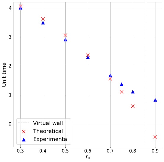
By comparing the looping times and computing the invariants, we validated our method on a nonlinear, pseudo-spectral simulation. This example also demonstrates the method at its full potential. Each simulation requires 30,000 iterations, which takes around 40 minutes to run on the same system as in § 3.2. The method solves a PDE involving Laplacian on a complex field with angular and radial modes below 0.1 s.
4 Conclusions and perspectives
This paper introduced a novel spectral method suited for Cauchy problems featuring Laplacians in polar coordinates. We reformulated the discrete Hankel transforms as pseudospectral methods, and we introduced DHTs’ quadrature weights, cardinal functions, and pseudospectral grids. We discussed the choice of sampling grids for both FFTs and DHTs, and analyzed the error bounds of the numerical interpolation and DHTs. We demonstrated a systematic way to use the method to compute Laplacians and apply spectral time schemes to time-dependent partial differential equations. We then showed a range of time-dependent examples including linear and nonlinear PDEs, fields with complex numbers, and the 2-D wave equation involving the second order time derivative. We verified the theoretical error bound on functions with different boundary conditions. The method was validated by comparing the simulation results with analytical solutions and by checking energy, mass, and angular momentum conservations. Although all our equations and examples are on unit disks throughout this paper for concision, the method can be rescaled to arbitrary radii Baddour2019; 2004_JOSAA_Guizar-SicairosG. We acknowledge that the literature has extensively studied the discretization of the Laplacian operator and Poisson-type equations in polar coordinates, employing finite difference methods, finite element methods, or alternative spectral methods with orthogonal polynomials. Many of these methods exhibit faster convergence rates, resulting in higher accuracy when computing Laplacians compared to the technique we present in this paper. Nevertheless, our method could potentially offer greater time marching efficiency due to the mathematically exact time marching scheme that utilizes eigenfunctions of the Laplacian (see § 2.4). However, a more detailed comparison is required to address this claim, and this also depends on the nonlinear parts.
A way to greatly speed up the method is to implement the program for parallel computing. After the FFT step, for which parallel libraries are widely available, each angular mode is independent of the others, and the following interpolations and DHTs can be distributed to different processes at the same time. Due to the nature of Bessel functions, the method converges poorly if the homogeneous Dirichlet condition is not satisfied. However, there are many known ways to homogenize boundary conditions BISWAS2019721; Friedman1997; Achdou1998, which may be combined with our method for more general problems. We are currently considering a new transform based on Dini series, a variation of the Fourier-Bessel series which works on Neumann and Robin boundary conditions (watson1995treatise, § 18.11). A combination of these transforms has the potential to compute Laplacians under arbitrary boundary conditions. Holman and Kunyansky suggest a reduced polar sampling grid Holman2015, which becomes more sparse towards the domain center. Our current sampling grid has redundancy in the inner part at high angular modes, and adopting their strategy may improve efficiency.
Acknowledgment
N.G. thanks the 2009 WHOI Geophysical Fluid Dynamics program on nonlinear waves and especially Oliver Bühler for fruitful scientific discussions.
References
- (1) M.C. Lai, W.W. Lin, W. Wang, A fast spectral/difference method without pole conditions for poisson-type equations in cylindrical and spherical geometries. IMA Journal of Numerical Analysis 22, 537–548 (2002). 10.1093/imanum/22.4.537
- (2) M.C. Lai, W.C. Wang, Fast direct solvers for poisson equation on 2d polar and spherical geometries. Numerical Methods for Partial Differential Equations 18, 56–68 (2002). 10.1002/num.1038
- (3) K. Mohseni, T. Colonius, Numerical Treatment of Polar Coordinate Singularities. Journal of Computational Physics 157(2), 787–795 (2000). 10.1006/jcph.1999.6382
- (4) B. Prochnow, O. O’Reilly, E.M. Dunham, N.A. Petersson, Treatment of the polar coordinate singularity in axisymmetric wave propagation using high-order summation-by-parts operators on a staggered grid. Computers and Fluids 149, 138–149 (2017). 10.1016/j.compfluid.2017.03.015
- (5) J.P. Boyd, F. Yu, Comparing seven spectral methods for interpolation and for solving the Poisson equation in a disk: Zernike polynomials, Logan-Shepp ridge polynomials, Chebyshev-Fourier Series, cylindrical Robert functions, Bessel-Fourier expansions, square-to-disk confor. Journal of Computational Physics 230(4), 1408–1438 (2011). 10.1016/j.jcp.2010.11.011
- (6) A.B. Bhatia, E. Wolf, On the circle polynomials of Zernike and related orthogonal sets. Mathematical Proceedings of the Cambridge Philosophical Society 50(1), 40–48 (1954). 10.1017/S0305004100029066
- (7) K. Atkinson, D. Chien, O. Hansen, A spectral method for elliptic equations: The Dirichlet problem. Advances in Computational Mathematics 33(2), 169–189 (2010). 10.1007/s10444-009-9125-8. arXiv:arXiv:0809.0021v1
- (8) J. Shen, New fast Chebyshev-Fourier algorithm for Poisson-type equations in polar geometries. Applied Numerical Mathematics 33(1), 183–190 (2000). 10.1016/S0168-9274(99)00082-3
- (9) T. Matsushima, P.S. Marcus, A spectral method for polar coordinates. Journal of Computational Physics 120(2), 365–374 (1995). 10.1006/jcph.1995.1171
- (10) G.M. Vasil, K.J. Burns, D. Lecoanet, S. Olver, B.P. Brown, J.S. Oishi, Tensor calculus in polar coordinates using Jacobi polynomials. Journal of Computational Physics 325, 53–73 (2016). 10.1016/j.jcp.2016.08.013. arXiv:1509.07624
- (11) G.N. Watson, A Treatise on the Theory of Bessel Functions. Cambridge Mathematical Library (Cambridge University Press, 1995), p. 134
- (12) N. Temme, An algorithm with ALGOL 60 program for the computation of the zeros of ordinary bessel functions and those of their derivatives. Journal of Computational Physics 32(2), 270–279 (1979). 10.1016/0021-9991(79)90134-7
- (13) N.F. Marshall, O. Mickelin, A. Singer. Fast expansion into harmonics on the disk: a steerable basis with fast radial convolutions (2022)
- (14) H.F. Johnson, An improved method for computing a discrete Hankel transform. Computer Physics Communications 43(2), 181–202 (1987). 10.1016/0010-4655(87)90204-9
- (15) L. Yu, M. Huang, M. Chen, W. Chen, W. Huang, Z. Zhu, Quasi-discrete Hankel transform. Opt. Lett. 23(6), 409–411 (1998). 10.1364/OL.23.000409
- (16) M. Guizar-Sicairos, J.C. Gutierrez-Vega, Computation of quasi-discrete Hankel transforms of integer order for propagating optical wave fields. Journal of the Optical Society of America A 21(1), 53 (2004). 10.1364/JOSAA.21.000053
- (17) N. Baddour, in Fourier Transforms - Century of Digitalization and Increasing Expectations, vol. 32, ed. by G.S. Nikolic, D.Z. Markovic-Nikolic (IntechOpen, London, UK, 2019), pp. 137–144. 10.5772/intechopen.84399
- (18) J.P. Boyd, Chebyshev and Fourier Spectral Methods: Second Revised Edition. Dover Books on Mathematics (Dover Publications, 2013)
- (19) J. Shen, T. Tang, L.L. Wang, Spectral Methods, Springer Series in Computational Mathematics, vol. 41 (Springer Berlin Heidelberg, Berlin, Heidelberg, 2011). 10.1007/978-3-540-71041-7
- (20) N. Baddour, Discrete two-dimensional fourier transform in polar coordinates part I: Theory and operational rules. Mathematics 7(8), 1–32 (2019). 10.3390/math7080698
- (21) X. Yao, N. Baddour, Discrete two dimensional Fourier Transform in polar coordinates Part II: Numerical computation and approximation of the continuous transform. PeerJ Computer Science 2020(3), 1–38 (2020). 10.7717/peerj-cs.257
- (22) C.A. Hall, W. Meyer, Optimal error bounds for cubic spline interpolation. Journal of Approximation Theory 16(2), 105–122 (1976). https://doi.org/10.1016/0021-9045(76)90040-X
- (23) L.J. Landau, Bessel functions: Monotonicity and bounds. Journal of the London Mathematical Society 61(1), 197–215 (2000). 10.1112/S0024610799008352
- (24) K. Toraichi, K. Katagishi, I. Sekita, R. Mori, Computational complexity of spline interpolation. International Journal of Systems Science 18(5), 945–954 (1987). 10.1080/00207728708964021
- (25) W. H., S.A. Teukolsky, W.T. Vetterling, B.P. Flannery, Numerical Recipes 3rd Edition: The Art of Scientific Computing, 3rd edn. (Cambridge University Press, USA, 2007)
- (26) C.L. Siegel, in On Some Applications of Diophantine Approximations: a translation of Carl Ludwig Siegel’s Über einige Anwendungen diophantischer Approximationen by Clemens Fuchs, with a commentary and the article Integral points on curves: Siegel’s theorem after Siegel’s proof by Clemens Fuchs and Umberto Zannier, ed. by U. Zannier (Scuola Normale Superiore, Pisa, 2014), pp. 81–138. 10.1007/978-88-7642-520-2_2
- (27) G.K. Batchelor, An Introduction to Fluid Dynamics. Cambridge Mathematical Library (Cambridge University Press, 2000). 10.1017/CBO9780511800955
- (28) N. Grisouard, in 2009 program of studies: nonlinear waves, ed. by O. Bühler, K. Helfrich (Woods Hole Oceanographic Institution, 2010), pp. 269–289. 10.1575/1912/3213
- (29) W. Bao, Q. Du, Y. Zhang, Dynamics of rotating bose-einstein condensates and its efficient and accurate numerical computation. SIAM Journal on Applied Mathematics 66, 758–786 (2006). 10.1137/050629392
- (30) W. Bao, H. Li, J. Shen, A generalized-laguerre-fourier-hermite pseudospectral method for computing the dynamics of rotating bose-einstein condensates. SIAM Journal on Scientific Computing 31, 3685–3711 (2009). 10.1137/080739811
- (31) W. Bao, Y. Cai, Mathematical theory and numerical methods for bose-einstein condensation. Kinetic and Related Models 6(1), 1–135 (2013). 10.3934/krm.2013.6.1. URL http://arxiv.org/abs/1212.5341http://dx.doi.org/10.3934/krm.2013.6.1
- (32) W. Bao, Q. Tang, Numerical study of quantized vortex interactions in the nonlinear schrödinger equation on bounded domains. Multiscale Modeling and Simulation 12, 411–439 (2014). 10.1137/130906489
- (33) E.P. Gross, Structure of a quantized vortex in boson systems. Nuovo Cimento 20, 454–477 (1960). 10.1007/BF02731494
- (34) L.P. Pitaevskii, Vortex lines in an imperfect Bose gas. Sov. Phys. JETP 13(2), 451–454 (1961)
- (35) Y. Guo, O. Bühler, Wave-vortex interactions in the nonlinear schrödinger equation. Physics of Fluids 26(2), 1–22 (2014). 10.1063/1.4865837
- (36) P. Mason, N.G. Berloff, A.L. Fetter, Motion of a vortex line near the boundary of a semi-infinite uniform condensate. Physical Review A - Atomic, Molecular, and Optical Physics 74 (2006). 10.1103/PhysRevA.74.043611
- (37) E. Madelung, Quantentheorie in hydrodynamischer Form. Zeitschrift für Physik 40(3), 322–326 (1927). 10.1007/BF01400372
- (38) P.K. Kundu, I.M. Cohen, D.R. Dowling, in Fluid Mechanics (Sixth Edition), ed. by P.K. Kundu, I.M. Cohen, D.R. Dowling, sixth edition edn. (Academic Press, Boston, 2016), pp. 195–226. https://doi.org/10.1016/B978-0-12-405935-1.00005-8
- (39) P. Biswas, S. Singh, H. Bindra, Homogenization of time dependent boundary conditions for multi-layer heat conduction problem in cylindrical polar coordinates. International Journal of Heat and Mass Transfer 129, 721–734 (2019). https://doi.org/10.1016/j.ijheatmasstransfer.2018.10.036
- (40) A. Friedman, B. Hu, A non-stationary multi-scale oscillating free boundary for the laplace and heat equations. Journal of Differential Equations 137(1), 119–165 (1997). 10.1016/S0022-0396(06)80006-9
- (41) Y. Achdou, P. Le Tallec, F. Valentin, O. Pironneau, Constructing wall laws with Domain Decomposition or asymptotic expansion techniques. Computer Methods in Applied Mechanics and Engineering 151(1-2), 215–232 (1998). 10.1016/S0045-7825(97)00118-7
- (42) B. Holman, L. Kunyansky, DRAFT A Second-order Finite Difference Scheme For The Wave Equation on a Reduced Polar Grid (2015). URL https://www.math.arizona.edu/˜leonk/papers/polarFD7.pdf. [Unpublished], Department of Mathematics, The University of Arizona
Appendix A Proof of
We prove the equality in Eqn. (20). By substituting the Fourier-Bessel expansion Eqn. (2) into the forward transform formula Eqn. (8), we have
| (41) |
We rearrange this expression into
| (42) |
Summing the above equation over the pseudospectral grid points , from the orthogonality relation (6), we find the expression we were looking for, namely,
| (43) |
Therefore, applying a DHT with radial modes is equivalent to truncating a Fourier-Bessel series at the term.