跳到论文正文
W Papers独立论文阅读器 arXiv:2210.09721 论文正文 计算阅读时间 · 0%
引用这篇论文根据当前论文元数据生成,正式投稿前建议核对。


License: arXiv.org perpetual non-exclusive license
arXiv:2210.09721v3 [eess.SY] 07 Nov 2023

An incremental input-to-state stability condition for a generic class of recurrent neural networks

William D’Amico    Alessio La Bella    Marcello Farina Thanks: The authors are with Dipartimento di Elettronica, Informazione e Bioingegneria, Politecnico di Milano, Via Ponzio 34/5, 20133, Milano, Italy (e-mail: william.damico@polimi.it, alessio.labella@polimi.it, and marcello.farina@polimi.it). Corresponding author: William D’Amico.
Abstract

This paper proposes a novel sufficient condition for the incremental input-to-state stability of a generic class of recurrent neural networks (RNNs). The established condition is compared with others available in the literature, showing to be less conservative. Moreover, it can be applied for the design of incremental input-to-state stable RNN-based control systems, resulting in a linear matrix inequality constraint for some specific RNN architectures. The formulation of nonlinear observers for the considered system class, as well as the design of control schemes with explicit integral action, are also investigated. The theoretical results are validated through simulation on a referenced nonlinear system.

Index Terms: 
Neural networks, linear matrix inequalities, nonlinear control systems, stability of nonlinear systems.

Neural networks (NNs) have gained interest in many engineering fields, given the ever-growing availability of large amounts of data, e.g., collected measurements from plants, and their significant ability to reproduce nonlinear dynamics [1, 2]. In particular, NNs have shown to be particularly suited for control applications, as they can be used not only to identify unknown systems, but also to directly design feedback controllers from data [3, 4]. Among existing NN architectures, recurrent neural networks (RNNs) are typically adopted for controlling dynamical systems, since they are inherently characterized by the presence of state variables [5].

Despite the increasing popularity of RNNs, their theoretical properties have been rarely analysed. As nonlinear dynamical systems, it is in fact fundamental to characterize conditions that guarantee the stability of their motions, especially when RNNs are part of control systems [6, 7]. In this context incremental input-to-state stability (δ\deltaISS) [8, 9] plays a crucial role. This property entails that, asymptotically, the state trajectories are solely determined by the applied inputs and not by their initial conditions [10]. Thus, the dynamics of a δ\deltaISS RNN is independent of its initialization. The δ\deltaISS property also enables the design of trivial observers for the RNN states: the latter, indeed, can be asymptotically estimated just exploiting the knowledge of the applied inputs. Finally, note that the δ\deltaISS implies other common stability properties, e.g., global asymptotic stability (GAS) of the equilibria and input-to-state stability (ISS) [10, 8].

Motivated by this, the paper presents a novel δ\deltaISS sufficient condition for a generic class of RNN architectures. The proposed condition is applicable to control systems, and in particular for the analysis and design of RNNs-based feedback controllers and feedforward compensators.

-A State of the art and contribution

Despite the large popularity and potentialities of RNNs in control applications, relatively few stability results have been discussed in the literature. Sufficient conditions ensuring stability-related properties for RNNs are presented in [11] and in [12], the latter focusing on a specific class of RNNs, i.e., gated recurrent units (GRU). A stability condition for a generic class of RNNs is discussed in [13], considering however the case with constant inputs. Note that the above-mentioned contributions address stability properties weaker than the δ\deltaISS (e.g., the GAS property), which do not consider the effect of inputs [8]. This has motivated other research studies to focus on conditions guaranteeing δ\deltaISS. The latter, interestingly, can be directly enforced in the data-based RNN training phase, e.g., as discussed in [14, 15]. However, these works focus on open-loop RNNs, and they do not address the design of stabilizing RNN-based feedback controllers.
Regarding control systems, in [16] the stability is analysed in case of feedforward NN (FFNN) controllers and assuming a linear controlled system with uncertainties. Design conditions for FFNN controllers are also provided in [17], considering specific classes of second-order nonlinear systems under control. Also model predictive control (MPC) has been investigated as a method for the design of efficient controllers applicable to systems described by specific classes of RNNs. For instance, the ISS of a MPC-controlled neural nonlinear autoregressive exogenous (NNARX) system is discussed in [18]. Also, MPC regulation strategies for other RNN architectures are presented in [19] and [20], ensuring closed-loop stability if the RNN-based model of the controlled system enjoys the δ\deltaISS property.

In this work we first derive a novel δ\deltaISS condition for a generic class of discrete-time nonlinear systems, which includes the one analysed in [21], as well as different common RNN classes (e.g., echo state networks and NNARX). We prove that the proposed condition is less conservative than existing ones established in the past years for RNNs, e.g., [14, 19, 13]. The established results turn out to be particularly suited for the design of feedback controllers and feedforward compensators. In particular, they allow us to enforce the δ\deltaISS property on control systems, also in case the controlled system does not enjoy the same property. Moreover, we show that, if specific RNN-based control architectures are considered, the design problem translates to a linear matrix inequality (LMI) problem, efficiently solvable by common solvers.

-B Paper outline

The paper is structured as follows. In Section I, the equations of the considered generic class of RNNs are introduced. The novel sufficient condition δ\deltaISS is stated in Section II and it is compared with other existing conditions in the literature. In Section III, the δ\deltaISS properties of feedforward and feedback interconnected RNNs are investigated, whereas Section IV discusses in details the controller design with δ\deltaISS guarantees. Section V shows the application of the theoretical results in this paper to a simulation example, whereas conclusions are drawn in Section VI.

-C Notation and basic definitions

Given a matrix AA, its transpose is ATA^{T}, and the transpose of its inverse is A−TA^{-T}. The entry in the ii-th row and jj-th column of a matrix AA is denoted as ai​ja_{ij}. |A||A| denotes a matrix whose entries are |ai​j||a_{ij}|, for all i,ji,j. The ii-th entry of a vector vv is indicated as viv_{i}. Given a symmetric matrix PP, we use P⪰0P\succeq 0, P≻0P\succ 0, P⪯0P\preceq 0, and P≺0P\prec 0 to indicate that it is positive semidefinite, positive definite, negative semidefinite, and negative definite, respectively. λm​i​n​(P)\lambda_{min}(P) and λm​a​x​(P)\lambda_{max}(P) denote the minimum and maximum eigenvalues of a symmetric matrix PP, respectively. 0n,m0_{n,m} denotes a zero matrix with nn rows and mm columns and InI_{n} is the identity matrix of dimension nn. Given a sequence of square matrices A1,A2,…,AnA_{1},A_{2},\dots,A_{n}, D=D= diag(A1,A2,…,An)(A_{1},A_{2},\dots,A_{n}) is a block diagonal matrix having A1,A2,…,AnA_{1},A_{2},\dots,A_{n} as sub-matrices on the main-diagonal blocks. Moreover, ‖v‖=vT​v\|v\|=\sqrt{v^{T}v} denotes the 2-norm of a column vector vv and ‖v‖Q=vT​Q​v\|v\|_{Q}=\sqrt{v^{T}Qv} denotes the weighted Euclidean norm of vv, where QQ is a positive definite matrix. Given a sequence u→=u⁡(0),u⁡(1),…\vec{u}=u(0),u(1),\dots, we define its infinity norm as ‖u→‖∞=supk∈ℕ‖u⁡(k)‖\|\vec{u}\|_{\infty}=\sup_{k\in\mathbb{N}}\|u(k)\|. Also, i​dn​(⋅)id_{n}(\cdot) denotes a column vector of dimension nn with all elements equal to the identity function i​d​(⋅)id(\cdot). We introduce the following definition.

Definition 1 (​​[22]).

A real function g:ℝ→ℝg:\mathbb{R}\to\mathbb{R} is called globally Lipschitz continuous if there exist a constant Lp≥0L_{p}\geq 0 such that, for any x,y∈ℝx,y\in\mathbb{R}, it holds that

|g⁡(x)−g⁡(y)|≤Lp​|x−y|.|g(x)-g(y)|\leq L_{p}|x-y|\,.

The following property will be used later in the paper.

Property 1 (​​[19]).

Given two vectors a,b∈ℝna,b\in\mathbb{R}^{n}, it holds that ‖a+b‖2≤(1+τ2)​‖a‖2+(1+1τ2)​‖b‖2\|a+b\|^{2}\leq(1+\tau^{2})\|a\|^{2}+\left(1+\frac{1}{\tau^{2}}\right)\|b\|^{2} for any scalar τ≠0\tau\neq 0.

We now consider a general discrete-time nonlinear system expressed as

x⁡(k+1)=fo​(x⁡(k),u⁡(k)),x(k+1)=f^{o}(x(k),u(k))\,, (1)

where fo:𝕏×𝕌→𝕏f^{o}:\mathbb{X}\times\mathbb{U}\to\mathbb{X}, 𝕏⊆ℝn\mathbb{X}\subseteq\mathbb{R}^{n}, 𝕌⊆ℝm\mathbb{U}\subseteq\mathbb{R}^{m}, 0n,1∈𝕏0_{n,1}\in\mathbb{X}, and 0m,1∈𝕌0_{m,1}\in\mathbb{U}. Moreover, fo​(⋅)f^{o}(\cdot) is such that fo​(0n,1,0m,1)=0n,1f^{o}(0_{n,1},0_{m,1})=0_{n,1}, k∈ℤ≥0k\in\mathbb{Z}_{\geq 0} is the discrete-time index, x⁡(k)∈𝕏x(k)\in\mathbb{X} is the state of the system and u⁡(k)∈𝕌u(k)\in\mathbb{U} is the exogenous variable. The set of admissible input sequences u→\vec{u} is denoted by 𝒰\mathcal{U}. We indicate with x⁡(k,x0,u→)x(k,x_{0},\vec{u}) the solution to the system (1) at time kk starting from the initial state x0∈𝕏x_{0}\in\mathbb{X} with input sequence u→∈𝒰\vec{u}\in\mathcal{U}.
Now, we recall some useful notions for the following (see [10]).

Definition 2 (𝒦\mathcal{K} function[10]).

A continuous function α:ℝ≥0→ℝ≥0\alpha:\mathbb{R}_{\geq 0}\to\mathbb{R}_{\geq 0} is a class 𝒦\mathcal{K} function if α⁡(s)>0\alpha(s)>0 for all s>0s>0, it is strictly increasing, and α⁡(0)=0\alpha(0)=0.

Definition 3 (𝒦∞\mathcal{K}_{\infty} function[10]).

A continuous function α:ℝ≥0→ℝ≥0\alpha:\mathbb{R}_{\geq 0}\to\mathbb{R}_{\geq 0} is a class 𝒦∞\mathcal{K}_{\infty} function if it is a class 𝒦\mathcal{K} function and α⁡(s)→∞\alpha(s)\to\infty for s→∞s\to\infty.

Definition 4 (𝒦​ℒ\mathcal{KL} function[10]).

A continuous function β:ℝ≥0×ℤ≥0→ℝ≥0\beta:\mathbb{R}_{\geq 0}\times\mathbb{Z}_{\geq 0}\to\mathbb{R}_{\geq 0} is a class 𝒦​ℒ\mathcal{KL} function if β⁡(s,k)\beta(s,k) is a class 𝒦\mathcal{K} function with respect to ss for all kk, it is strictly decreasing in kk for all s>0s>0, and β⁡(s,k)→0\beta(s,k)\to 0 as k→∞k\to\infty for all s>0s>0.

Definition 5 (δ\deltaISS[10]).

System (1) is called incrementally input-to-state stable if there exists a function β∈𝒦​ℒ\beta\in\mathcal{KL} and a function γ∈𝒦∞\gamma\in\mathcal{K}_{\infty} such that for any k∈ℤ≥0k\in\mathbb{Z}_{\geq 0}, any initial states x01,x02∈𝕏x_{01},x_{02}\in\mathbb{X}, and any couple of input sequences u→1,u→2∈𝒰\vec{u}_{1},\vec{u}_{2}\in\mathcal{U}, it holds that

∥x(k,x01,u→1)−x(k,x02,u→2)∥≤β(∥x01\displaystyle\|x(k,x_{01},\vec{u}_{1})-x(k,x_{02},\vec{u}_{2})\|\leq\beta(\|x_{01} −x02∥,k)+γ(∥u→1−u→2∥∞),\displaystyle-x_{02}\|,k)+\gamma(\|\vec{u}_{1}-\vec{u}_{2}\|_{\infty})\,,

where x⁡(k,x0​i,u→i)x(k,x_{0i},\vec{u}_{i}), i=1,2i=1,2, is the state of system (1) at time step kk, computed from the initial condition x0​i∈𝕏x_{0i}\in\mathbb{X} and with the input trajectory u→i∈𝒰\vec{u}_{i}\in\mathcal{U}.

Definition 6 (Dissipation-form δ\deltaISS Lyapunov function[9]).

A function V:𝕏×𝕏→ℝ≥0V:\mathbb{X}\times\mathbb{X}\to\mathbb{R}_{\geq 0} is called a dissipation-form δ\deltaISS-Lyapunov function for (1), if there exist functions ξ1,ξ2,ξ∈𝒦∞\xi_{1},\xi_{2},\xi\in\mathcal{K}_{\infty} and σ∈𝒦\sigma\in\mathcal{K} so that, for all x1,x2∈𝕏x_{1},x_{2}\in\mathbb{X} and u1,u2∈𝕌u_{1},u_{2}\in\mathbb{U}, it holds that

ξ1​(‖x1−x2‖)≤V⁡(x1,x2)≤ξ2​(‖x1−x2‖),\xi_{1}(\|x_{1}-x_{2}\|)\leq V(x_{1},x_{2})\leq\xi_{2}(\|x_{1}-x_{2}\|)\,, (2)
V⁡(f⁡(x1,u1),f⁡(x2,u2))−V⁡(x1,x2)≤−ξ⁡(‖x1−x2‖)+σ⁡(‖u1−u2‖).\begin{split}V(f(x_{1},u_{1}),f(x_{2},u_{2}))-V(x_{1},x_{2})\leq-\,\xi(\|x_{1}-x_{2}\|)+\,\sigma(\|u_{1}-u_{2}\|)\,.&\end{split} (3)
Theorem 1 (​​[9]).

If system (1) admits a dissipation-form δ\deltaISS Lyapunov function, then it is δ\deltaISS.

I Problem statement

We consider the following class of nonlinear discrete-time systems:

x⁡(k+1)\displaystyle x(k+1) =f⁡(A​x​(k)+B​u​(k)),\displaystyle=f(Ax(k)+Bu(k))\,, (4a)
y⁡(k)\displaystyle y(k) =C​x​(k)+D​u​(k),\displaystyle=Cx(k)+Du(k)\,, (4b)

where u⁡(k)∈ℝmu(k)\in\mathbb{R}^{m} is the exogenous variable, y⁡(k)∈ℝly(k)\in\mathbb{R}^{l} is the output vector, x⁡(k)∈ℝnx(k)\in\mathbb{R}^{n} is the state vector, f⁡(⋅)=[f1​(⋅)…fn​(⋅)]T∈ℝnf(\cdot)=\begin{bmatrix}f_{1}(\cdot)&\dots&f_{n}(\cdot)\end{bmatrix}^{T}\in\mathbb{R}^{n} is a vector of scalar functions applied element-wise, A∈ℝn×nA\in\mathbb{R}^{n\times n}, B∈ℝn×mB\in\mathbb{R}^{n\times m}, C∈ℝl×nC\in\mathbb{R}^{l\times n}, and D∈ℝl×mD\in\mathbb{R}^{l\times m}. The exogenous variable u⁡(k)u(k) takes different roles in the various setups considered in this paper. Namely, u⁡(k)u(k) can be the manipulable input variable in case of open-loop systems, whereas it can be the output reference or the exogenous disturbance in case of closed-loop control systems. In this work, the function f⁡(⋅)f(\cdot) takes the particular form specified in the following assumption.

Assumption 1.

The functions fi​(⋅)f_{i}(\cdot), i=1,…,ni=1,\dots,n, are nonlinear globally Lipschitz continuous functions with Lipschitz constant Lp​iL_{pi}, or the identity function i​d​(⋅)id(\cdot).

Given a system in class (4), let us introduce the set

ℒ={i∈{1,…,n}|fi​(⋅)≠i​d​(⋅)}.\mathcal{L}\!=\!\{i\in\{1,\dots,n\}\,|\;f_{i}(\cdot)\!\neq\!id(\cdot)\}\,.

Note that, under Assumption 1, system (4) is representative of several RNN architectures. For instance, (4) includes the general formulation of RNNs considered in [21], where D=0l,mD=0_{l,m}, f1​(⋅)=⋯=fn​(⋅)=σf​(⋅)f_{1}(\cdot)=\dots=f_{n}(\cdot)=\sigma_{f}(\cdot), and σf:ℝ→ℝ\sigma_{f}:\mathbb{R}\to\mathbb{R} is a globally Lipschitz function (e.g., rectified linear unit (ReLU), sigmoid, or tanh\tanh). Also, as better clarified below, many other RNNs considered in the literature can be written in form (4), possibly under some assumptions and/or minor reformulations.

I-A Example 1: echo state networks (ESNs)

ESNs [23] are particular types of RNNs composed of a dynamical reservoir (hidden layer) in which the connections between neurons are sparse and random. If we consider the formulation proposed in [19], with ν\nu neurons (i.e., states) in the reservoir, input u⁡(k)∈ℝmu(k)\in\mathbb{R}^{m}, output y⁡(k)∈ℝly(k)\in\mathbb{R}^{l}, nonlinear Lipschitz continuous internal units output functions ζ⁡(⋅)\zeta(\cdot) applied element-wise, and linear output units output functions, the ESN equations are:

χ⁡(k+1)\displaystyle\chi(k+1) =ζ⁡(Wx​χ​(k)+Wu​u​(k)+Wy​y​(k)),\displaystyle=\zeta(W_{x}\chi(k)+W_{u}u(k)+W_{y}y(k))\,, (5a)
y⁡(k)\displaystyle y(k) =Wo​u​t1​χ​(k)+Wo​u​t2​u​(k−1),\displaystyle=W_{out_{1}}\chi(k)+W_{out_{2}}u(k-1)\,, (5b)

where Wx∈ℝν×νW_{x}\in\mathbb{R}^{\nu\times\nu}, Wu∈ℝν×mW_{u}\in\mathbb{R}^{\nu\times m}, Wy∈ℝν×lW_{y}\in\mathbb{R}^{\nu\times l}, Wo​u​t1∈ℝl×νW_{out_{1}}\in\mathbb{R}^{l\times\nu}, and Wo​u​t2∈ℝl×mW_{out_{2}}\in\mathbb{R}^{l\times m}.
Note that model (5) can be reformulated as (4) by defining x⁡(k)=[χ​(k)Tz​(k)T]Tx(k)=\begin{bmatrix}\chi(k)^{T}&z(k)^{T}\end{bmatrix}^{T}, where z⁡(k)=u⁡(k−1)z(k)=u(k-1), and by setting

A=[Wx∗Wy​Wo​u​t20m,ν0m,m],\displaystyle A=\left[\begin{matrix}W_{x}^{*}&W_{y}W_{out_{2}}\\ 0_{m,\nu}&0_{m,m}\end{matrix}\right], (6)

B=[WuTIm]TB=\begin{bmatrix}W_{u}^{T}&I_{m}\end{bmatrix}^{T}, C=[Wo​u​t1Wo​u​t2]C=\begin{bmatrix}W_{out_{1}}&W_{out_{2}}\end{bmatrix}, D=0l,mD=0_{l,m}, and f⁡(⋅)=[ζ​(⋅)Ti​dm​(⋅)T]Tf(\cdot)=\begin{bmatrix}\zeta(\cdot)^{T}&id_{m}(\cdot)^{T}\end{bmatrix}^{T}, where Wx∗=Wx+Wy​Wo​u​t1W_{x}^{*}=W_{x}+W_{y}W_{out_{1}}.

I-B Example 2: shallow neural nonlinear autoregressive exogenous (NNARX) models

NNARX is a class of nonlinear autoregressive exogenous models where a FFNN is used as nonlinear regression function. As shown in [14], a shallow (i.e., 1-layer) NNARX, with input u~​(k)∈ℝm~\tilde{u}(k)\in\mathbb{R}^{\widetilde{m}}, output y⁡(k)∈ℝly(k)\in\mathbb{R}^{l}, and ν\nu neurons, is a dynamical system defined by the following equation

y⁡(k+1)=W0​ζ​(Wϕ​ϕ​(k)+Wu​u~​(k)+b)+b0,y(k+1)=W_{0}\zeta(W_{\phi}\phi(k)+W_{u}\tilde{u}(k)+b)+b_{0}\,, (7)

where W0∈ℝl×νW_{0}\in\mathbb{R}^{l\times\nu}, b0∈ℝlb_{0}\in\mathbb{R}^{l}, the vector ϕ⁡(k)∈ℝ(l+m~)​N\phi(k)\in\mathbb{R}^{(l+\widetilde{m})N} is defined as

ϕ(k)=[\displaystyle\phi(k)=\big[ u~(k−N)T,y(k−N+1)T,…,u~(k−2)T,y(k−1)T,u~(k−1)T,y(k)T]T,\displaystyle\tilde{u}(k-N)^{T},y(k-N+1)^{T},...\,,\tilde{u}(k-2)^{T},y(k-1)^{T},\tilde{u}(k-1)^{T},\,y(k)^{T}\,\big]^{T}\,, (8)

ζ⁡(⋅)∈ℝν\zeta(\cdot)\in\mathbb{R}^{\nu} is a vector of Lipschitz continuous activation functions applied element-wise, Wu∈ℝν×m~W_{u}\in\mathbb{R}^{\nu\times\widetilde{m}}, b∈ℝνb\in\mathbb{R}^{\nu}, Wϕ=[Wϕ1Wϕ2Wϕ3]∈ℝν×(m~+l)​NW_{\phi}=\begin{bmatrix}W_{\phi_{1}}&W_{\phi_{2}}&W_{\phi_{3}}\end{bmatrix}\in\mathbb{R}^{\nu\times(\widetilde{m}+l)N}, Wϕ1∈ℝν×(m~+l)W_{\phi_{1}}\in\mathbb{R}^{\nu\times(\widetilde{m}+l)}, Wϕ2∈ℝν×τW_{\phi_{2}}\in\mathbb{R}^{\nu\times\tau}, τ=(l+m~)​N−2​l−m~\tau=(l+\widetilde{m})N-2l-\widetilde{m}, and Wϕ3∈ℝν×lW_{\phi_{3}}\in\mathbb{R}^{\nu\times l}.

Proposition 1.

Model (7) can be reformulated as (4) by defining u⁡(k)=[u~​(k)T1]Tu(k)=\begin{bmatrix}\tilde{u}(k)^{T}&1\end{bmatrix}^{T},

x⁡(k)=[ϕ~​(k)T,υ​(k)T]T,\displaystyle x(k)=\big[\,\widetilde{\phi}(k)^{T},\;\upsilon(k)^{T}\,\big]^{T}\,, (9)

where

ϕ~​(k)\displaystyle\widetilde{\phi}(k) =[u~​(k−N)T,y​(k−N+1)T,…,u~​(k−2)T,y​(k−1)T,u~​(k−1)T]T,\displaystyle=\big[\tilde{u}(k-N)^{T},y(k-N+1)^{T},...\,,\tilde{u}(k-2)^{T},y(k-1)^{T},\tilde{u}(k-1)^{T}\big]^{T}\,,
υ⁡(k)\displaystyle\upsilon(k) =ζ⁡(Wϕ​ϕ​(k−1)+Wu​u~​(k−1)+b),\displaystyle=\zeta(W_{\phi}\phi(k-1)+W_{u}\tilde{u}(k-1)+b)\,,

and by setting

A\displaystyle A =[0τ,l+m~Iτ0τ,ν0l,l+m~0l,τW00m~,l+m~0m~,τ0m~,νWϕ1Wϕ2Wϕ3​W0],\displaystyle=\left[\begin{matrix}0_{\tau,l+\widetilde{m}}&I_{\tau}&0_{\tau,\nu}\\ 0_{l,l+\widetilde{m}}&0_{l,\tau}&W_{0}\\ 0_{\widetilde{m},l+\widetilde{m}}&0_{\widetilde{m},\tau}&0_{\widetilde{m},\nu}\\ W_{\phi_{1}}&W_{\phi_{2}}&W_{\phi_{3}}W_{0}\end{matrix}\right]\,, (10)
B\displaystyle B =[0τ,m~0τ,10l,m~b0Im~0m~,1Wub+Wϕ3​b0],\displaystyle=\left[\begin{matrix}0_{\tau,\widetilde{m}}&0_{\tau,1}\\ 0_{l,\widetilde{m}}&b_{0}\\ I_{\widetilde{m}}&0_{\widetilde{m},1}\\ W_{u}&b+W_{\phi_{3}}b_{0}\end{matrix}\right]\,, (11)

C=[0l,n−νW0]C=\begin{bmatrix}0_{l,n-\nu}&W_{0}\end{bmatrix}, D=[0l,m~b0]D=\begin{bmatrix}0_{l,\widetilde{m}}&b_{0}\end{bmatrix}, and f⁡(⋅)=[i​dn−ν​(⋅)Tζ​(⋅)T]Tf(\cdot)=\begin{bmatrix}id_{n-\nu}(\cdot)^{T}&\zeta(\cdot)^{T}\end{bmatrix}^{T}.

Proof.

Let us consider the extended input u⁡(k)u(k) and the extended state vector x⁡(k)∈ℝnx(k)\in\mathbb{R}^{n}, with n=ν+(l+m~)​N−ln=\nu+(l+\widetilde{m})N-l. Firstly, note that

ϕ~​(k+1)=[0τ,l+m~Iτ0τ,ν0l,l+m~0l,τW00m~,l+m~0m~,τ0m~,ν]​x​(k)+[0τ,m~0τ,10l,m~b0Im~0m~,1]​u​(k).\displaystyle\widetilde{\phi}(k\!+\!1)\!=\!\left[\begin{matrix}0_{\tau,l+\widetilde{m}}\!&\!I_{\tau}\!&\!0_{\tau,\nu}\\ 0_{l,l+\widetilde{m}}\!&\!0_{l,\tau}\!&\!W_{0}\\ 0_{\widetilde{m},l+\widetilde{m}}\!&\!0_{\widetilde{m},\tau}\!&\!0_{\widetilde{m},\nu}\end{matrix}\right]\!x(k)\!+\!\left[\begin{matrix}0_{\tau,\widetilde{m}}\!&\!0_{\tau,1}\\ 0_{l,\widetilde{m}}\!&\!b_{0}\\ I_{\widetilde{m}}\!&\!0_{\widetilde{m},1}\end{matrix}\right]\!u(k).

Secondly,

υ⁡(k+1)\displaystyle\upsilon(k+1) =ζ⁡(Wϕ​ϕ​(k)+Wu​u~​(k)+b)=\displaystyle=\zeta(W_{\phi}\phi(k)+W_{u}\tilde{u}(k)+b)=
=ζ⁡([Wϕ1Wϕ2]​ϕ~​(k)+Wϕ3​y​(k)+Wu​u~​(k)+b)=\displaystyle=\zeta(\begin{bmatrix}W_{\phi_{1}}\!&\!W_{\phi_{2}}\end{bmatrix}\!\widetilde{\phi}(k)\!+\!W_{\phi_{3}}y(k)+W_{u}\tilde{u}(k)+b)=
=ζ⁡([Wϕ1Wϕ2]​ϕ~​(k)+Wϕ3​W0​υ​(k)+Wϕ3​b0+Wu​u~​(k)+b)\displaystyle=\zeta(\begin{bmatrix}W_{\phi_{1}}\!&\!W_{\phi_{2}}\end{bmatrix}\!\widetilde{\phi}(k)\!+\!W_{\phi_{3}}\!W_{0}\upsilon(k)\!+\!W_{\phi_{3}}\!b_{0}\!+\!W_{u}\tilde{u}(k)\!+\!b)

This concludes the proof of the statement. ∎

I-C Example 3: class of RNN systems in [13]

In [13] a slightly different RNN class is considered, i.e.,

x⁡(k+1)=E​x​(k)+O​f​(A^​x​(k)+s),\displaystyle x(k+1)=Ex(k)+O\,f(\hat{A}x(k)+s)\,, (12)

where A^\hat{A} is a full matrix, E=diag​(e1,…,en)E=\text{diag}(e_{1},\dots,e_{n}), O=diag​(o1,…,on)O=\text{diag}(o_{1},\dots,o_{n}), s=[s1…sn]Ts=\begin{bmatrix}s_{1}&\dots&s_{n}\end{bmatrix}^{T} is a vector of constant inputs, with ei,oi,si∈ℝe_{i},\,o_{i},\,s_{i}\in\mathbb{R}, ∀i=1,…,n\forall i=1,\dots,n. Moreover, f⁡(⋅)=[f1​(⋅)…fn​(⋅)]Tf(\cdot)=\begin{bmatrix}f_{1}(\cdot)&\dots&f_{n}(\cdot)\end{bmatrix}^{T}, where each fi​(⋅)f_{i}(\cdot) is a globally Lipschitz continuous activation function with Lipschitz constant Lp​iL_{pi}. Note that, in case E=0n,nE=0_{n,n} and oi=1o_{i}=1 for all i∈ℒi\in\mathcal{L}, system (12) is in the same form of (4a).

Given the generic class of systems (4) under Assumption 1, a sufficient condition ensuring the δ\deltaISS property is established and described in the following section.

II A novel sufficient condition for incremental input-to-state stability of RNNs

Let us consider a generic system (4) fulfilling Assumption 1. The following theorem provides a sufficient condition which guarantees the δ\deltaISS for nonlinear systems lying in the class (4a). We first define a diagonal matrix W=diag​(Lp​1,…,Lp​n)∈ℝn×nW=\text{diag}(L_{p1},\dots,L_{pn})\in\mathbb{R}^{n\times n}, where Lp​i=1L_{pi}=1 for all i∉ℒi\notin\mathcal{L}. We introduce the matrices A~=W​A\widetilde{A}=WA and B~=W​B\widetilde{B}=WB.

Theorem 2.

Let Assumption 1 hold. System (4a) is δ\deltaISS if ∃P=PT≻0\exists P=P^{T}\succ 0 such that pi​j=pj​i=0p_{ij}=p_{ji}=0 ∀i∈ℒ\forall i\!\in\!\mathcal{L}, ∀j∈{1,…,n}\forall j\!\in\!\{1,\dots,n\} with j≠ij\neq i, and

A~T​P​A~−P≺0.\displaystyle\widetilde{A}^{T}P\widetilde{A}-P\prec 0\,. (13)
Proof.

In order to prove the δ\deltaISS of system (4a) we show the existence of a dissipation-form δ\deltaISS Lyapunov function. We consider, as candidate, V⁡(x1​(k),x2​(k))=‖x1​(k)−x2​(k)‖P2V(x_{1}(k),x_{2}(k))=\|x_{1}(k)-x_{2}(k)\|^{2}_{P}.

From now on, for notational simplicity, we drop the dependence on kk. If we consider the 𝒦∞\mathcal{K}_{\infty} functions ξ1​(‖x1−x2‖)=λm​i​n​(P)​‖x1−x2‖2\xi_{1}(\|x_{1}-x_{2}\|)=\lambda_{min}(P)\|x_{1}-x_{2}\|^{2} and ξ2​(‖x1−x2‖)=λm​a​x​(P)​‖x1−x2‖2\xi_{2}(\|x_{1}-x_{2}\|)=\lambda_{max}(P)\|x_{1}-x_{2}\|^{2}, condition (2) is easily verified. To prove that V⁡(x1,x2)V(x_{1},x_{2}) satisfies also condition (3), we introduce the following notation: v1=A​x1+B​u1v_{1}=Ax_{1}+Bu_{1}, x1+=f⁡(v1)x_{1}^{+}=f(v_{1}), v2=A​x2+B​u2v_{2}=Ax_{2}+Bu_{2}, x2+=f⁡(v2)x_{2}^{+}=f(v_{2}), δ​x=x1−x2\delta x=x_{1}-x_{2}, δ​x+=x1+−x2+\delta x^{+}=x_{1}^{+}-x_{2}^{+}, and δ​u=u1−u2\delta u=u_{1}-u_{2}. We can write

δ​x+\displaystyle\delta x^{+} =f⁡(v1)−f⁡(v2)=\displaystyle=f(v_{1})-f(v_{2})=
=W​v1−W​v2+f⁡(v1)−W​v1−f⁡(v2)+W​v2=\displaystyle=Wv_{1}-Wv_{2}+f(v_{1})-Wv_{1}-f(v_{2})+Wv_{2}=
=A~​δ​x+B~​δ​u+Δ,\displaystyle=\widetilde{A}\delta x+\widetilde{B}\delta u\,\,+\Delta\,, (14)

where Δ=f⁡(v1)−W​v1−f⁡(v2)+W​v2\Delta=f(v_{1})-Wv_{1}-f(v_{2})+Wv_{2}. From (14), we obtain that

V⁡(x1+,x2+)−V⁡(x1,x2)\displaystyle V(x_{1}^{+},x_{2}^{+})-V(x_{1},x_{2}) =(δ​x+)T​P​δ​x+−δ​xT​P​δ​x=\displaystyle=(\delta x^{+})^{T}P\delta x^{+}-\delta x^{T}P\delta x=
=(A~​δ​x+B~​δ​u)T​P​(A~​δ​x+B~​δ​u)+2​(A~​δ​x+B~​δ​u)T​P​Δ+ΔT​P​Δ−δ​xT​P​δ​x.\displaystyle=(\widetilde{A}\delta x+\widetilde{B}\delta u)^{T}P(\widetilde{A}\delta x+\widetilde{B}\delta u)+2(\widetilde{A}\delta x+\widetilde{B}\delta u)^{T}P\Delta\,+\Delta^{T}P\Delta-\delta x^{T}P\delta x\,. (15)

Now, we can observe that

2​(A~​δ​x+B~​δ​u)T​P​Δ+ΔT​P​Δ\displaystyle 2(\widetilde{A}\delta x+\widetilde{B}\delta u)^{T}P\Delta+\Delta^{T}P\Delta =2​(W⁡(v1−v2))T​P​Δ+ΔT​P​Δ=\displaystyle=2(W(v_{1}-v_{2}))^{T}P\Delta+\Delta^{T}P\Delta=
=(2​W​v1−2​W​v2+Δ)T​P​Δ=\displaystyle=(2Wv_{1}-2Wv_{2}+\Delta)^{T}P\Delta=
=qT​P​r,\displaystyle=q^{T}Pr\,, (16)

where q,r∈ℝnq,r\in\mathbb{R}^{n}, with q=W​v1+f⁡(v1)−W​v2−f⁡(v2)q=Wv_{1}+f(v_{1})-Wv_{2}-f(v_{2}) and r=f⁡(v1)−W​v1−f⁡(v2)+W​v2r=f(v_{1})-Wv_{1}-f(v_{2})+Wv_{2}. The elements of the vectors qq and rr are

qi={fi​(v1​i)−fi​(v2​i)+Lp​i​(v1​i−v2​i)if​i∈ℒ,2​v1​i−2​v2​iif​i∉ℒ,\centering q_{i}=\left\{\begin{split}&f_{i}(v_{1i})-f_{i}(v_{2i})+L_{pi}(v_{1i}-v_{2i})\hskip 14.22636pt&\text{if}\;i\in\mathcal{L}\,,\\ &2v_{1i}-2v_{2i}&\text{if}\;i\notin\mathcal{L}\,,\\ \end{split}\right.\@add@centering
ri={fi​(v1​i)−fi​(v2​i)−Lp​i​(v1​i−v2​i)if​i∈ℒ,0if​i∉ℒ.\centering r_{i}=\left\{\begin{split}&f_{i}(v_{1i})-f_{i}(v_{2i})-L_{pi}(v_{1i}-v_{2i})\hskip 14.22636pt&\text{if}\;i\in\mathcal{L}\,,\\ &0&\text{if}\;i\notin\mathcal{L}\,.\\ \end{split}\right.\@add@centering

Therefore, by setting pi​j=pj​i=0p_{ij}=p_{ji}=0 ∀i∈ℒ\forall i\!\in\!\mathcal{L} and ∀j∈{1,…,n}\forall j\!\in\!\{1,\dots,n\} with j≠ij\neq i, we can compute from (16) that

qT​P​r=∑i∈ℒpi​i​((fi​(v1​i)−fi​(v2​i))2−Lp​i2​(v1​i−v2​i)2)≤0.\displaystyle q^{T}Pr=\!\sum_{i\in\mathcal{L}}p_{ii}\left((f_{i}(v_{1i})-f_{i}(v_{2i}))^{2}-\!L_{pi}^{2}(v_{1i}-v_{2i})^{2}\right)\leq 0\,. (17)

Inequality (17) holds since, in view of Assumption 1, fi​(⋅)f_{i}(\cdot) are globally Lipschitz continuous functions, for all i∈ℒi\in\mathcal{L}, and pi​i>0p_{ii}>0 ∀i\forall i since P=PT≻0P=P^{T}\succ 0.

As a result, by exploiting (17) and in view of Property 1, for any τ≠0\tau\neq 0, we can write that

V⁡(x1+,x2+)−V⁡(x1,x2)\displaystyle V(x_{1}^{+},x_{2}^{+})-V(x_{1},x_{2}) ≤(A~​δ​x+B~​δ​u)T​P​(A~​δ​x+B~​δ​u)−δ​xT​P​δ​x≤\displaystyle\leq(\widetilde{A}\delta x+\widetilde{B}\delta u)^{T}P(\widetilde{A}\delta x+\widetilde{B}\delta u)-\delta x^{T}P\delta x\leq
≤(1+τ2)​(A~​δ​x)T​P​A~​δ​x+(1+1τ2)​(B~​δ​u)T​P​B~​δ​u−δ​xT​P​δ​x≤\displaystyle\leq(1+\tau^{2})(\widetilde{A}\delta x)^{T}P\widetilde{A}\delta x+\left(1+\frac{1}{\tau^{2}}\right)(\widetilde{B}\delta u)^{T}P\widetilde{B}\delta u-\delta x^{T}P\delta x\leq
≤−λm​i​n​(A∗)​‖x1−x2‖2+λu​‖u1−u2‖2,\displaystyle\leq-\lambda_{min}(A^{*})\|x_{1}-x_{2}\|^{2}+\lambda_{u}\|u_{1}-u_{2}\|^{2}\,,

for any λu>λm​a​x​(B∗)\lambda_{u}>\lambda_{max}(B^{*}), where A∗=P−(1+τ2)​A~T​P​A~≻0A^{*}=P-(1+\tau^{2})\widetilde{A}^{T}P\widetilde{A}\succ 0 in view of (13) for a sufficiently small τ\tau, and B∗=(1+1τ2)​B~T​P​B~⪰0B^{*}=\left(1+\frac{1}{\tau^{2}}\right)\widetilde{B}^{T}P\widetilde{B}\succeq 0.

Finally, note that σ⁡(‖u1−u2‖)=λu​‖u1−u2‖2\sigma(\|u_{1}-u_{2}\|)=\lambda_{u}\|u_{1}-u_{2}\|^{2} is a 𝒦\mathcal{K} function, whereas ξ⁡(‖x1−x2‖)=λm​i​n​(A∗)​‖x1−x2‖2\xi(\|x_{1}-x_{2}\|)=\lambda_{min}(A^{*})\|x_{1}-x_{2}\|^{2} is a 𝒦∞\mathcal{K}_{\infty} function. This concludes the proof. ∎

In short, Theorem 2 ensures that system (4a) is δ\deltaISS if A~\widetilde{A} is Schur stable and if there exists a matrix PP with a specific structure fulfilling the Lyapunov inequality (13). In particular, PP must have zero elements along all the rows and columns (except for the diagonal element) corresponding to the rows of (4a) whose activation function is nonlinear.

The δ\deltaISS condition in Theorem 2 is now compared with other existing conditions for the RNN systems introduced in Section I to show its generality.

II-A Comparison with the stability condition in [19] for ESNs

Note that, in case of ESNs, the assumptions of Theorem 2 require the existence of a positive definite block diagonal matrix P=diag​(P1,P2)P=\text{diag}(P_{1},P_{2}) fulfilling (13), where P1∈ℝν×νP_{1}\in\mathbb{R}^{\nu\times\nu} is a diagonal matrix, as ℒ={1,…,ν}\mathcal{L}=\{1,\dots,\nu\}, and P2∈ℝm×mP_{2}\in\mathbb{R}^{m\times m} is a full symmetric matrix. On the other hand, in [19, Proposition 1] the following sufficient condition for δ\deltaISS of system (5) in state-space is proposed in case ζ⁡(⋅)\zeta(\cdot) has activation functions with Lipschitz constant Lp≤1L_{p}\leq 1.

Proposition 2 (​​[19]).

If ‖Wx∗‖<1\|W_{x}^{*}\|<1, system (5) in the state-space form in [19] is δ\deltaISS.

Below we show that the assumptions of Theorem 2 are less conservative than the one of Proposition 2.

Proposition 3.

Let ζ⁡(⋅)\zeta(\cdot) be a vector of sigmoid Lipschitz continuous functions with Lipschitz constant Lp≤1L_{p}\leq 1. The set of systems (5) satisfying the assumption of Proposition 2 is a subset of the set of systems (5) satisfying the assumptions of Theorem 2.

Proof.

See the Appendix. ∎

We also show an example in which the assumption of Proposition 2 is not fulfilled whereas the assumptions of Theorem 2 are. Let ν=2\nu=2, m=1m=1, l=1l=1,

Wx=[0.8257−0.4711−1.01490.137],Wy=[−0.29190.3018],W_{x}=\left[\begin{matrix}0.8257&-0.4711\\ -1.0149&0.137\end{matrix}\right]\,,\ \ \ W_{y}=\left[\begin{matrix}-0.2919\\ 0.3018\end{matrix}\right]\,,

Wo​u​t1=[0.3999−0.93]W_{out_{1}}=\begin{bmatrix}0.3999&-0.93\end{bmatrix}, and Wo​u​t2=−0.1768W_{out_{2}}=-0.1768. Then, ‖Wx∗‖=1.1413>1\|W_{x}^{*}\|=1.1413>1. With AA defined as in (6) and with the choice

P=[2.14440000.72210001.0254],P=\left[\begin{matrix}2.1444&0&0\\ 0&0.7221&0\\ 0&0&1.0254\\ \end{matrix}\right]\,,

we have that the maximum eigenvalue of AT​P​A−PA^{T}PA-P is equal to −0.3197-0.3197, and thus AT​P​A−P≺0A^{T}PA-P\prec 0.

II-B Comparison with the stability condition in [14] for shallow NNARX models

In case of shallow NNARXs, the assumptions of Theorem 2 require the existence of a symmetric positive definite matrix PP fulfilling (13) such that pi​j=pj​i=0p_{ij}=p_{ji}=0, ∀i∈ℒ={n−ν+1,…,n}\forall i\in\mathcal{L}=\{n-\nu+1,\dots,n\} and ∀j∈{1,…,n}\forall j\in\{1,\dots,n\} with j≠ij\neq i.

In [14, Theorem 8] a sufficient condition for δ\deltaISS of a deep (i.e., MM-layered) NNARX is proposed. For comparison purposes, we recall here the condition for a 1-layer NNARX (7), as this belongs to the class (4), where ζ⁡(⋅)\zeta(\cdot) has activation functions with Lipschitz constant LpL_{p}. Note also that, in [14], a slightly different state-space formulation with respect to the one in this paper is considered.

Proposition 4 (​​[14]).

If ‖W0‖​‖Wϕ‖<1Lp​N\|W_{0}\|\|W_{\phi}\|<\frac{1}{L_{p}\sqrt{N}}, system (7) in the state-space form in [14] is δ\deltaISS.

Below we show that the assumptions of Theorem 2 are less conservative than the one of Proposition 4 for a shallow NNARX.

Proposition 5.

Let ζ⁡(⋅)\zeta(\cdot) be a vector of nonlinear Lipschitz continuous functions with Lipschitz constant LpL_{p}. The set of systems (7) satisfying the assumption of Proposition 4 is a subset of the set of systems (7) satisfying the assumptions of Theorem 2.

Proof.

See the Appendix. ∎

Here we show an example in which the assumption of Proposition 4 is not fulfilled whereas the assumptions of Theorem 2 hold. Let l=1l=1, m~=1\widetilde{m}=1, N=2N=2, ν=1\nu=1, Lp=1L_{p}=1, Wϕ=[−0.2130−0.8657−1.0431−0.2701]W_{\phi}=\left[\begin{matrix}-0.2130&-0.8657&-1.0431&-0.2701\end{matrix}\right] and W0=0.6293W_{0}=0.6293. Then, ‖W0‖​‖Wϕ‖=0.8801>0.7071=1N\|W_{0}\|\|W_{\phi}\|=0.8801>0.7071=\frac{1}{\sqrt{N}}. With the choice

P=[0.82780.00950.184700.00951.22580.753100.18470.75312.587000000.8723],P=\left[\begin{matrix}0.8278&0.0095&0.1847&0\\ 0.0095&1.2258&0.7531&0\\ 0.1847&0.7531&2.5870&0\\ 0&0&0&0.8723\end{matrix}\right]\,,

we have that the maximum eigenvalue of A~T​P​A~−P\widetilde{A}^{T}P\widetilde{A}-P is equal to −0.239-0.239 and, thus, A~T​P​A~−P≺0\widetilde{A}^{T}P\widetilde{A}-P\prec 0.

II-C Comparison with the stability condition in [13] for a class of RNN systems

The work in [13] analyses the stability properties of a slightly different RNN class represented by (12). In [13, Corollary 1] some sufficient conditions for global exponential stability are proposed. Among them, the following condition has a similar structure to the one of Theorem 2, and it is thus compared.

Proposition 6 (​​[13]).

System (12) is globally exponentially stable for any input ss if there exists a matrix P=PT≻0P\!=\!P^{T}\!\succ\!0 such that

M^T​P​M^−P≺0,\displaystyle\hat{M}^{T}P\hat{M}-P\prec 0\,, (18)

where M^=|E|+W​|O|​|A^|\hat{M}=|E|\,+\,W|O||\hat{A}|, and W=diag​(Lp​1,…,Lp​n)W=\text{diag}(L_{p1},\dots,L_{pn}).

For the sake of comparison, we now show that the assumptions of Theorem 2 are less conservative than the one of Proposition 6 for the class of RNN systems (12) with E=0n,nE=0_{n,n} and oi=1o_{i}=1 ∀i∈ℒ\forall i\in\mathcal{L}. Therefore, the following proposition is stated.

Proposition 7.

The set of systems (12) satisfying the assumption of Proposition 6 is a subset of the set of systems (12) satisfying the assumptions of Theorem 2 if E=0n,nE=0_{n,n} and oi=1o_{i}=1 ∀i∈ℒ\forall i\in\mathcal{L}.

Proof.

See the Appendix. ∎

Here we show an example in which the assumption of Proposition 6 is not fulfilled whereas the ones of Theorem 2 hold. Let n=2n=2, E=02,2E=0_{2,2}, O=I2O=I_{2}, W=I2W=I_{2}, ℒ={1,2}\mathcal{L}=\{1,2\},

A^=[0.4178−0.85440.81990.3573].\hat{A}=\left[\begin{matrix}0.4178&-0.8544\\ 0.8199&0.3573\end{matrix}\right].

Hence, the spectral radius of M^\hat{M} is equal to 1.2251.225 and so (18) is never fulfilled. With the choice

P=[1.2122001.2657],P=\left[\begin{matrix}1.2122&0\\ 0&1.2657\end{matrix}\right]\,,

we have that the maximum eigenvalue of A~T​P​A~−P\widetilde{A}^{T}P\widetilde{A}-P is equal to −0.1135-0.1135 and, thus, A~T​P​A~−P≺0\widetilde{A}^{T}P\widetilde{A}-P\prec 0.

III δ\deltaISS of interconnected RNNs

We now show how Theorem 2 also applies to the interconnection of systems in class (4).

III-A Feedforward interconnection

In this section we investigate the δ\deltaISS conditions of the series of MsM_{s} systems lying in the class (4). Specifically, each system is numbered in increasing order with respect to ii and defined by

xi​(k+1)\displaystyle x_{i}(k+1) =fsi​(Ai​xi​(k)+Bi​ui​(k)),\displaystyle=f_{s_{i}}(A_{i}x_{i}(k)+B_{i}u_{i}(k))\,, (19a)
yi​(k)\displaystyle y_{i}(k) =Ci​xi​(k)+Di​ui​(k),\displaystyle=C_{i}x_{i}(k)+D_{i}u_{i}(k)\,, (19b)

where ui​(k)∈ℝmiu_{i}(k)\in\mathbb{R}^{m_{i}}, yi​(k)∈ℝliy_{i}(k)\in\mathbb{R}^{l_{i}}, and xi​(k)∈ℝnix_{i}(k)\in\mathbb{R}^{n_{i}}. Because of the series interconnection, it holds that ui​(k)=yi−1​(k)u_{i}(k)=y_{i-1}(k), for all i=2,…,Msi=2,...,M_{s}, and the following assumption is required to have dimensional consistency,

Assumption 2.

We assume that the dimension of ui​(k)u_{i}(k) is the same of yi−1​(k)y_{i-1}(k), i.e., mi=li−1m_{i}=l_{i-1}, for all i=2,…,Msi=2,...,M_{s}.

We can state the following result.

Proposition 8.

Let Assumption 2 hold. The series of MsM_{s} systems in the class (4) lies in the class (4).

Proof.

Firstly, note that the input of the first subsystem is the input of the overall series interconnection, i.e., u​(k)=u1​(k)u(k)=u_{1}(k), whereas the output of the last subsystem of the series is the overall output, i.e., y​(k)=yMs​(k)y(k)=y_{M_{s}}(k). Since yi​(k)=ui−1​(k)y_{i}(k)=u_{i-1}(k), for all i=2,…,Msi=2,...,M_{s}, due to the series interconnection and under Assumption 2, the second subsystem can be written as

x2​(k+1)=fs2​(A2​x2​(k)+B2​C1​x1​(k)+B2​D1​u​(k)),y2​(k)=C2​x2​(k)+D2​C1​x1​(k)+D2​D1​u​(k).\displaystyle\begin{split}x_{2}(k+1)&=f_{s_{2}}(A_{2}x_{2}(k)+B_{2}C_{1}x_{1}(k)+B_{2}D_{1}u(k))\,,\\ y_{2}(k)&=C_{2}x_{2}(k)+D_{2}C_{1}x_{1}(k)+D_{2}D_{1}u(k)\,.\end{split} (20)

Following the same reasoning, for i=3,…,Msi=3,...,M_{s}, it holds that

xi​(k+1)\displaystyle x_{i}(k+1) =fsi​(Bi​(∑h=1i−2(∏j=0i−h−2Di−1−j)​Ch​xh​(k))+Bi​Ci−1​xi−1​(k)+Ai​xi​(k)+Bi​(∏j=0i−2Di−1−j)​u​(k)),\displaystyle=f_{s_{i}}\big(B_{i}(\sum_{h=1}^{i-2}(\prod_{j=0}^{i-h-2}D_{i-1-j})C_{h}x_{h}(k))+B_{i}C_{i-1}x_{i-1}(k)+A_{i}x_{i}(k)+B_{i}(\prod_{j=0}^{i-2}D_{i-1-j})u(k))\,, (21a)
yi​(k)\displaystyle y_{i}(k) =∑h=1i−1(∏j=0i−h−1Di−j)​Ch​xh​(k)+Ci​xi​(k)+(∏j=0i−1Di−j)​u​(k).\displaystyle=\sum_{h=1}^{i-1}(\prod_{j=0}^{i-h-1}D_{i-j})C_{h}x_{h}(k)+C_{i}x_{i}(k)+(\prod_{j=0}^{i-1}D_{i-j})u(k)\,. (21b)

From (19)-(20)-(21), by introducing the extended state vector x⁡(k)=[x1​(k)T…xMs​(k)T]Tx(k)=\begin{bmatrix}x_{1}(k)^{T}&\dots&x_{M_{s}}(k)^{T}\end{bmatrix}^{T}, it is possible to construct the matrices AA, BB, CC, DD and the vector f⁡(⋅)=[fs1​(⋅)T…fsMs​(⋅)T]Tf(\cdot)=\begin{bmatrix}f_{s_{1}}(\cdot)^{T}&\dots&f_{s_{M_{s}}}(\cdot)^{T}\end{bmatrix}^{T} of the overall system in the form (4). This concludes the proof. ∎

To guarantee the δ\deltaISS of the series of MsM_{s} systems in the form (4), one way is to write the overall series system as (4), and then to impose the sufficient condition for δ\deltaISS in Theorem 2 to the overall system. Alternatively, we can impose the sufficient condition for δ\deltaISS in Theorem 2 to each subsystem. In [8, Proposition 4.7], a theoretical result proves that the series interconnection of two δ\deltaISS continuous-time systems is δ\deltaISS. The same property can be extended to discrete-time systems. In the following Proposition 9 we show that, given a series of discrete-time systems each one satisfying the assumptions of Theorem 2 for δ\deltaISS, their series interconnection satisfies the same assumptions.

Proposition 9.

Let us consider a series of systems in the class (4), each one fulfilling the assumptions of Theorem 2. The series of these systems satisfies the assumptions of Theorem 2.

Proof.

See the Appendix. ∎

III-B Feedback interconnection

Refer to caption
Fig. 1: Feedback control scheme: 𝒞\mathcal{C} is the controller, 𝒮\mathcal{S} is the system to be controlled, rr is the reference signal, ee is the tracking error, usu_{s} is the manipulated variable, and ysy_{s} is the output of the system.

In this section we investigate the δ\deltaISS conditions of the feedback of two systems lying in the class (4). The baseline feedback control scheme is depicted in Figure 1. We define the equations of the controller 𝒞\mathcal{C} as

xc​(k+1)\displaystyle x_{c}(k+1) =fc​(Ac​xc​(k)+Bc​uc​(k)),\displaystyle=f_{c}(A_{c}x_{c}(k)+B_{c}u_{c}(k))\,, (22a)
yc​(k)\displaystyle y_{c}(k) =Cc​xc​(k)+Dc​uc​(k),\displaystyle=C_{c}x_{c}(k)+D_{c}u_{c}(k)\,, (22b)

where uc​(k)∈ℝmcu_{c}(k)\in\mathbb{R}^{m_{c}}, yc​(k)∈ℝlcy_{c}(k)\in\mathbb{R}^{l_{c}}, and xc​(k)∈ℝncx_{c}(k)\in\mathbb{R}^{n_{c}}. We consider the case in which the system is strictly proper to avoid algebraic loops. Thus, we define the equations of the controlled system 𝒮\mathcal{S} as

xs​(k+1)\displaystyle x_{s}(k+1) =fs​(As​xs​(k)+Bs​us​(k)),\displaystyle=f_{s}(A_{s}x_{s}(k)+B_{s}u_{s}(k))\,, (23a)
ys​(k)\displaystyle y_{s}(k) =Cs​xs​(k),\displaystyle=C_{s}x_{s}(k)\,, (23b)

where us​(k)∈ℝmsu_{s}(k)\in\mathbb{R}^{m_{s}}, ys​(k)∈ℝlsy_{s}(k)\in\mathbb{R}^{l_{s}}, and xs​(k)∈ℝnsx_{s}(k)\in\mathbb{R}^{n_{s}}. The following assumption is required to have dimensional consistency.

Assumption 3.

We assume that the dimension of us​(k)u_{s}(k) is the same of yc​(k)y_{c}(k), and the one of uc​(k)u_{c}(k) is the same of ys​(k)y_{s}(k), i.e., ms=lcm_{s}=l_{c} and mc=lsm_{c}=l_{s}.

We can state the following result.

Proposition 10.

Let Assumption 3 hold. The feedback interconnection in Figure 1 of the systems (22)-(23) in the class (4) lies in the class (4).

Proof.

Firstly, note from Figure 1 that r⁡(k)r(k) is overall input to the feedback interconnection, i.e., u⁡(k)=r⁡(k)u(k)=r(k), whereas ys​(k)y_{s}(k) is the overall output, i.e., y​(k)=ys​(k)y(k)=y_{s}(k). Under Assumption 3, since uc​(k)=e⁡(k)=r⁡(k)−ys​(k)=r⁡(k)−Cs​xs​(k)u_{c}(k)=e(k)=r(k)-y_{s}(k)=r(k)-C_{s}x_{s}(k) due to the negative feedback interconnection, and us​(k)=yc​(k)=Cc​xc​(k)+Dc​uc​(k)u_{s}(k)=y_{c}(k)=C_{c}x_{c}(k)+D_{c}u_{c}(k), we can write the equations of the overall closed-loop system in the formulation (4) through the following definitions:

A=[Ac−Bc​CsBs​CcAs−Bs​Dc​Cs],B=[BcBs​Dc],\displaystyle A=\left[\begin{matrix}A_{c}&-B_{c}C_{s}\\ B_{s}C_{c}&A_{s}-B_{s}D_{c}C_{s}\end{matrix}\right]\,,\ \ \ B=\left[\begin{matrix}B_{c}\\ B_{s}D_{c}\end{matrix}\right]\,,

C=[0ls,ncCs]C=\begin{bmatrix}0_{l_{s},n_{c}}&C_{s}\end{bmatrix}, D=0ls,lsD=0_{l_{s},l_{s}}, x⁡(k)=[xc​(k)Txs​(k)T]Tx(k)=\begin{bmatrix}x_{c}(k)^{T}&x_{s}(k)^{T}\end{bmatrix}^{T}, and f⁡(⋅)=[fc​(⋅)Tfs​(⋅)T]Tf(\cdot)=\begin{bmatrix}f_{c}(\cdot)^{T}&f_{s}(\cdot)^{T}\end{bmatrix}^{T}. ∎

It is possible to show that the previous result holds also for the case in which the controller is strictly proper and the system is not. We omit the proof for the sake of conciseness.

In view of Proposition 10 and Theorem 2, it is possible to analyse or enforce (through the tuning of the parameters of 𝒞\mathcal{C}) the δ\deltaISS property to the feedback control scheme in Figure 1, where both the controller and the system are in the class (4).

IV Controller design with δ\deltaISS guarantees

This section discusses the design of controllers that confer δ\deltaISS guarantees to the control system. In this paper, we will not focus on the performances of the control system, which will be a matter of future research.

In general, the δ\deltaISS condition (13) in Theorem 2 corresponds to a nonlinear constraint in control design, which can be handled by common nonlinear solvers. On the other hand, there are some particular cases in which it can be reformulated as a linear matrix inequality (LMI) constraint, as shown in the following section.

IV-A LMI-based control design

We consider a control system whose overall equations are in the class (4). In this section we show that, in some particular cases, the matrix AA of the closed-loop system can be written as A=F+G​JA=F+GJ, or as A=F+J​GA=F+JG, where FF and GG are known matrices depending on the system to be controlled, and JJ is a matrix to be tuned taking the role of the control gain. Therefore, the objective is to tune JJ so that the closed-loop system enjoys the δ\deltaISS property. In this respect, the following results hold.

Proposition 11.

Let us consider a system with equations in the class (4), where A=F+G​JA=F+GJ. Let F~=W​F\widetilde{F}=WF and G~=W​G\widetilde{G}=WG, where W=diag​(Lp​1,…,Lp​n)W=\text{diag}(L_{p1},\dots,L_{pn}) is the diagonal matrix defined in Section II. If ∃P=PT\exists P=P^{T}, having the structure required by Theorem 2, and ∃H\exists H such that

[P(F~​P+G~​H)TF~​P+G~​HP]≻0,\displaystyle\begin{bmatrix}P&(\widetilde{F}P+\widetilde{G}H)^{T}\\ \widetilde{F}P+\widetilde{G}H&P\end{bmatrix}\succ 0\,, (24)

then, if we set J=H​P−1J=HP^{-1}, the system (4) is δ\deltaISS.

Proof.

Firstly, note that from (24) it follows that P≻0P\succ 0 and P−1≻0P^{-1}\succ 0. Secondly, by resorting to the Schur complement, it holds that

P−(F~​P+G~​H)T​P−1​(F~​P+G~​H)≻0,\displaystyle P-(\widetilde{F}P+\widetilde{G}H)^{T}P^{-1}(\widetilde{F}P+\widetilde{G}H)\succ 0\,,

Since H=J​PH=JP, then we can write

P​(F~+G~​J)T​P−1​(F~+G~​J)​P−P​P−1​P\displaystyle P(\widetilde{F}+\widetilde{G}J)^{T}P^{-1}(\widetilde{F}+\widetilde{G}J)P-PP^{-1}P ≺0,\displaystyle\prec 0\,,
P⁡((F~+G~​J)T​P−1​(F~+G~​J)−P−1)​P\displaystyle P((\widetilde{F}+\widetilde{G}J)^{T}P^{-1}(\widetilde{F}+\widetilde{G}J)-P^{-1})P ≺0,\displaystyle\prec 0\,,
A~T​P−1​A~−P−1\displaystyle\widetilde{A}^{T}P^{-1}\widetilde{A}-P^{-1} ≺0,\displaystyle\prec 0\,, (25)

where A~=F~+G~​J\widetilde{A}=\widetilde{F}+\widetilde{G}J. Note that P−1=P−T≻0P^{-1}=P^{-T}\succ 0 is a matrix with the same structure of PP. From (25), the assumptions of Theorem 2 hold, concluding the proof. ∎

Proposition 12.

Let us consider a system with equations in the class (4), where A=F+J​GA=F+JG. Let F~=W​F\widetilde{F}=WF, where W=diag​(Lp​1,…,Lp​n)W=\text{diag}(L_{p1},\dots,L_{pn}) is the diagonal matrix defined in Section II and Lp​i>0L_{pi}>0 ∀i\forall i. If ∃P=PT\exists P=P^{T}, having the structure required by Theorem 2, and ∃H\exists H such that

[P−F~T​P​F~−GT​HT​F~−F~T​H​GGT​HTH​GP]≻0,\displaystyle\begin{bmatrix}P-\widetilde{F}^{T}P\widetilde{F}-G^{T}H^{T}\widetilde{F}-\widetilde{F}^{T}HG&G^{T}H^{T}\\ HG&P\end{bmatrix}\succ 0\,, (26)

then, if we set J=W−1​P−1​HJ=W^{-1}P^{-1}H, the system (4) is δ\deltaISS.

Proof.

Firstly, note that from (26) it follows that P≻0P\succ 0. Secondly, by resorting to the Schur complement, it holds that

P−F~T​P​F~−GT​HT​F~−F~T​H​G−GT​HT​P−1​H​G≻0,\displaystyle P-\widetilde{F}^{T}P\widetilde{F}-G^{T}H^{T}\widetilde{F}-\widetilde{F}^{T}HG-G^{T}H^{T}P^{-1}HG\succ 0\,,

Since H=P​J~H=P\widetilde{J}, where J~=W​J\widetilde{J}=WJ, then we can write

F~T​P​F~+GT​J~T​P​F~+F~T​P​J~​G+GT​J~T​P​J~​G−P\displaystyle\widetilde{F}^{T}P\widetilde{F}+G^{T}\widetilde{J}^{T}P\widetilde{F}+\widetilde{F}^{T}P\widetilde{J}G+G^{T}\widetilde{J}^{T}P\widetilde{J}G-P ≺0,\displaystyle\prec 0\,,
A~T​P​A~−P\displaystyle\widetilde{A}^{T}P\widetilde{A}-P ≺0,\displaystyle\prec 0\,, (27)

where A~=F~+J~​G\widetilde{A}=\widetilde{F}+\widetilde{J}G. From (27), the assumptions of Theorem 2 hold, concluding the proof. ∎

Now, we will show some examples of control design problems which can be solved using the results in Propositions 11 and 12. Note that, if JJ is a full matrix whose elements are the controller parameters, then HH is a full matrix as well. However, if JJ is a block matrix containing some zero blocks, then further constraints on the structure of the matrices HH and PP must be considered, as we will see in some of the following examples.

Example 1. Static linear state-feedback controller

We consider the problem of designing a state-feedback gain matrix KK such that the control system in Figure 2 enjoys δ\deltaISS. The equations of the system are defined as in (23). In this example the equation of the controller is

us​(k)=K​xs​(k)+u0​(k),u_{s}(k)=Kx_{s}(k)+u_{0}(k)\,, (28)

where K∈ℝms×nsK\in\mathbb{R}^{{m_{s}}\times n_{s}}, u0​(k)∈ℝmsu_{0}(k)\in\mathbb{R}^{m_{s}} is a suitable feedforward term possibly depending upon the reference signal, and the state xs​(k)x_{s}(k) is measurable or can be estimated by a suitable observer. Note that the state is certainly known in case it depends only on current and past input and output samples, e.g., a shallow NNARX where W0W_{0} and b0b_{0} are a priori selected and W0W_{0} is invertible. In [19], in case of ESNs, a possible observer is proposed. More generally, some insights about the design of suitable observers for generic systems in the class (4) are provided in Section IV-B.

Refer to caption
Fig. 2: State-feedback control scheme: KK is the state-feedback gain matrix, 𝒮\mathcal{S} is the system to be controlled, ysy_{s} is the output of the system, xsx_{s} is the state of the system, u0u_{0} is the feedforward term, uK=K​xsu_{K}=Kx_{s}, and usu_{s} is the manipulated variable.

Hence, the closed-loop system has equations in the class (4), where A=As+Bs​KA=A_{s}+B_{s}K has the structure required by Proposition 11 with F=AsF=A_{s}, G=BsG=B_{s}, and J=KJ=K.

Example 2. Echo state dynamic output-feedback controller

We consider the problem of designing an output-feedback controller for the control scheme in Figure 1, where the system lies in the class (23) and the controller is described by an ESN. We define the equations of the controller as

xc​(k+1)\displaystyle x_{c}(k+1) =ζc​(Wxc​xc​(k)+We​e​(k)+Wyc​yc​(k)),\displaystyle=\zeta_{c}(W_{x_{c}}x_{c}(k)+W_{e}e(k)+W_{y_{c}}y_{c}(k))\,, (29a)
yc​(k)\displaystyle y_{c}(k) =Wo​u​t1c​xc​(k),\displaystyle=W_{out_{1_{c}}}x_{c}(k)\,, (29b)

where the direct dependence of the input in the output equation is omitted, i.e., Wo​u​t2c=0lc,mcW_{out_{2_{c}}}=0_{l_{c},m_{c}}. By recalling that us​(k)=yc​(k)u_{s}(k)=y_{c}(k) and e⁡(k)=r⁡(k)−ys​(k)e(k)=r(k)-y_{s}(k), the equations of the overall closed-loop system are in the class (4), where x⁡(k)=[xc​(k)Txs​(k)T]Tx(k)=\begin{bmatrix}x_{c}(k)^{T}&x_{s}(k)^{T}\end{bmatrix}^{T}, f⁡(⋅)=[ζc​(⋅)Tfs​(⋅)T]Tf(\cdot)=\begin{bmatrix}\zeta_{c}(\cdot)^{T}&f_{s}(\cdot)^{T}\end{bmatrix}^{T}, C=[0ls,ncCs]C=\begin{bmatrix}0_{l_{s},n_{c}}&C_{s}\end{bmatrix}, D=0ls,lsD=0_{l_{s},l_{s}},

A=[Wxc+Wyc​Wo​u​t1c−We​CsBs​Wo​u​t1cAs],B=[We0ns,ls],\displaystyle A=\left[\begin{matrix}W_{x_{c}}+W_{y_{c}}W_{out_{1_{c}}}&-W_{e}C_{s}\\ B_{s}W_{out_{1_{c}}}&A_{s}\end{matrix}\right]\,,\ \ B=\left[\begin{matrix}W_{e}\\ 0_{n_{s},l_{s}}\end{matrix}\right]\,,

y​(k)=ys​(k)y(k)=y_{s}(k) is the overall output, and u⁡(k)=r⁡(k)u(k)=r(k) is the overall input. Since the system matrices are known and the matrices of the controller in the state equation are randomly generated, the only unknown matrix is Wo​u​t1cW_{out_{1_{c}}}. Hence, it is possible to write A=F+G​JA=F+GJ, where J=[Wo​u​t1c0lc,ns]J=\begin{bmatrix}W_{out_{1_{c}}}&0_{l_{c},n_{s}}\end{bmatrix},

F=[Wxc−We​Cs0ns,ncAs],G=[WycBs].\displaystyle F=\left[\begin{matrix}W_{x_{c}}&-W_{e}C_{s}\\ 0_{n_{s},n_{c}}&A_{s}\end{matrix}\right]\,,\ \ G=\left[\begin{matrix}W_{y_{c}}\\ B_{s}\end{matrix}\right]\,.

Therefore, it is possible to apply the result in Proposition 11. However, in order to obtain a JJ with the required structure, it is necessary to further constrain (i) the structure of the matrix HH, i.e., H=[H~0lc,ns]H=\begin{bmatrix}\widetilde{H}&0_{l_{c},n_{s}}\end{bmatrix}, where H~∈ℝlc×nc\widetilde{H}\in\mathbb{R}^{l_{c}\times n_{c}} is a free variable, and (ii) the structure of the matrix PP, i.e., P=PT=diag​(P1,P2)P=P^{T}=\text{diag}(P_{1},P_{2}), where, in turn, P1∈ℝnc×ncP_{1}\in\mathbb{R}^{n_{c}\times n_{c}} is diagonal, and P2∈ℝns×nsP_{2}\in\mathbb{R}^{n_{s}\times n_{s}} has the structure required by Theorem 2.

Example 3. Shallow NNARX dynamic output-feedback controller

We consider the problem of designing an output-feedback controller for the control scheme in Figure 1, where the system lies in the class (23) and the controller is described by a shallow NNARX (7). We use the subscript cc to denote the matrices and dimensions of the controller. For simplicity, we set bc=0νc,1b_{c}=0_{\nu_{c},1} and b0c=0lc,1b_{0_{c}}=0_{l_{c},1}, which is reasonable in case normalized data are considered. We also assume that W0cW_{0_{c}} is a priori selected, whereas Wϕc=[Wϕ1cWϕ2cWϕ3c]W_{\phi_{c}}=\begin{bmatrix}W_{\phi_{1_{c}}}&W_{\phi_{2_{c}}}&W_{\phi_{3_{c}}}\end{bmatrix} and WucW_{u_{c}} are the controller unknown matrices to be tuned. Note that the controller can be written in the state-space representation (22), where xc​(k)x_{c}(k) is defined as in (9), AcA_{c} as in (10), Bc=[0τc,mcT0lc,mcTImcWucT]TB_{c}=\left[\begin{matrix}0_{\tau_{c},m_{c}}^{T}&0_{l_{c},m_{c}}^{T}&I_{m_{c}}&W_{u_{c}}^{T}\end{matrix}\right]^{T}, Cc=[0lc,nc−νcW0c]C_{c}=\begin{bmatrix}0_{l_{c},n_{c}-\nu_{c}}&W_{0_{c}}\end{bmatrix}, Dc=0lc,mcD_{c}=0_{l_{c},m_{c}}, fc​(⋅)=[i​dnc−νc​(⋅)Tζc​(⋅)T]Tf_{c}(\cdot)=\begin{bmatrix}id_{n_{c}-\nu_{c}}(\cdot)^{T}&\zeta_{c}(\cdot)^{T}\end{bmatrix}^{T}, and uc​(k)=e⁡(k)=r⁡(k)−ys​(k)u_{c}(k)=e(k)=r(k)-y_{s}(k). By recalling that us​(k)=yc​(k)u_{s}(k)=y_{c}(k), the equations of the overall closed-loop system are in the class (4), where x⁡(k)=[xs​(k)Txc​(k)T]Tx(k)=\begin{bmatrix}x_{s}(k)^{T}&x_{c}(k)^{T}\end{bmatrix}^{T}, f⁡(⋅)=[fs​(⋅)Tfc​(⋅)T]Tf(\cdot)=\begin{bmatrix}f_{s}(\cdot)^{T}&f_{c}(\cdot)^{T}\end{bmatrix}^{T}, C=[Cs0ls,nc]C=\begin{bmatrix}C_{s}&0_{l_{s},n_{c}}\end{bmatrix}, D=0ls,lsD=0_{l_{s},l_{s}},

A=[AsBs​Cc−Bc​CsAc],B=[0ns,lsBc],\displaystyle A=\left[\begin{matrix}A_{s}&B_{s}C_{c}\\ -B_{c}C_{s}&A_{c}\end{matrix}\right]\,,\ \ B=\left[\begin{matrix}0_{n_{s},l_{s}}\\ B_{c}\end{matrix}\right]\,,

y​(k)=ys​(k)y(k)=y_{s}(k) is the overall output, and u⁡(k)=r⁡(k)u(k)=r(k) is the overall input. Hence, it is possible to write A=F+J​GA=F+JG, where

F=[AsBs​Cc[0τc,ns0lc,ns−Cs0νc,ns][0τc,lc+mcIτc0τc,νc0lc,lc+mc0lc,τcW0c0ls,lc+mc0ls,τc0ls,νc0νc,lc+mc0νc,τc0νc,νc]],G=[−Cs0ls,nc0nj2−ls,ns[Inc−νc0nc−νc,νc0lc,nc−νcW0c]],J=[0nj1,nj2[WucWϕc]],\displaystyle F=\begin{bmatrix}A_{s}&B_{s}C_{c}\\ \begin{bmatrix}0_{\tau_{c},n_{s}}\\ 0_{l_{c},n_{s}}\\ -C_{s}\\ 0_{\nu_{c},n_{s}}\end{bmatrix}&\begin{bmatrix}0_{\tau_{c},l_{c}+m_{c}}&I_{\tau_{c}}&0_{\tau_{c},\nu_{c}}\\ 0_{l_{c},l_{c}+m_{c}}&0_{l_{c},\tau_{c}}&W_{0_{c}}\\ 0_{l_{s},l_{c}+m_{c}}&0_{l_{s},\tau_{c}}&0_{l_{s},\nu_{c}}\\ 0_{\nu_{c},l_{c}+m_{c}}&0_{\nu_{c},\tau_{c}}&0_{\nu_{c},\nu_{c}}\end{bmatrix}\end{bmatrix}\,,\ \ \ G=\begin{bmatrix}-C_{s}&0_{l_{s},n_{c}}\\ 0_{n_{j_{2}}-l_{s},n_{s}}&\begin{bmatrix}I_{n_{c}-\nu_{c}}&0_{n_{c}-\nu_{c},\nu_{c}}\\ 0_{l_{c},n_{c}-\nu_{c}}&W_{0_{c}}\end{bmatrix}\end{bmatrix}\,,\ \ \ J=\begin{bmatrix}0_{n_{j_{1}},n_{j_{2}}}\\ \begin{bmatrix}W_{u_{c}}&W_{\phi_{c}}\end{bmatrix}\end{bmatrix}\,,

nj1=ns+nc−νcn_{j_{1}}=n_{s}+n_{c}-\nu_{c}, and nj2=(mc+lc)​Nc+mcn_{j_{2}}=(m_{c}+l_{c})N_{c}+m_{c}. Therefore, it is possible to apply the result in Proposition 12. However, in order to obtain a JJ with the required structure, it is necessary to further constrain (i) the structure of the matrix HH, i.e., H=[0nj1,nj2TH~T]TH=\begin{bmatrix}0_{n_{j_{1}},n_{j_{2}}}^{T}&\widetilde{H}^{T}\end{bmatrix}^{T}, where H~∈ℝνc×nj2\widetilde{H}\in\mathbb{R}^{\nu_{c}\times n_{j_{2}}} is a free variable, and (ii) the structure of the matrix PP, i.e., P=PT=diag​(P1,P2)P=P^{T}=\text{diag}(P_{1},P_{2}), where, in turn, P1∈ℝnj1×nj1P_{1}\in\mathbb{R}^{n_{j_{1}}\times n_{j_{1}}} and P2∈ℝνc×νcP_{2}\in\mathbb{R}^{\nu_{c}\times\nu_{c}} are matrices with the structure required by Theorem 2.

IV-B Observer design

In general, if the state is not measurable, the application of state-feedback control schemes (e.g., the one in Figure 2) requires the availability of a state estimate. For a system in class (4), the following observer is proposed to provide a reliable estimate x^\hat{x} of the state xx, based on the input-output measures uu and yy:

x^​(k+1)\displaystyle\hat{x}(k+1) =f⁡(A​x^​(k)+B​u​(k)+L⁡(y⁡(k)−y^​(k)))\displaystyle=f(A\hat{x}(k)+Bu(k)+L(y(k)-\hat{y}(k))) (30a)
y^​(k)\displaystyle\hat{y}(k) =C​x^​(k)+D​u​(k)\displaystyle=C\hat{x}(k)+Du(k) (30b)

where LL is the observer gain to be designed according to the following result.

Proposition 13.

Let us consider a system with equations in the class (4). Let us define the diagonal matrix

W=diag​(Lp​1,…,Lp​n)W=\text{diag}(L_{p1},\dots,L_{pn})

as specified in Section II. If the observer (30) is employed, with LL such that

[1λm​a​x​(W)2​In(A−L​C)TA−L​CIn]≻0,\displaystyle\begin{bmatrix}\frac{1}{\lambda_{max}(W)^{2}}I_{n}&(A-LC)^{T}\\ A-LC&I_{n}\end{bmatrix}\succ 0\,, (31)

then x^​(k)→x​(k)\hat{x}(k)\to x(k) as k→+∞k\to+\infty.

Proof.

Firstly, note that the dynamics of the estimation error is defined as e​(k)=x​(k)−x^​(k)e(k)=x(k)-\hat{x}(k). By jointly considering (4) and (30), the 2-norm of the estimation error at time instant k+1k+1 can be written as

‖e⁡(k+1)‖\displaystyle\|e(k+1)\| =∥f(Ax(k)+Bu(k))−f(Ax^(k)+Bu(k)+L(Cx(k)+Du(k)−(Cx^(k)+Du(k)))∥.\displaystyle=\|f(Ax(k)+Bu(k))-f(A\hat{x}(k)+Bu(k)+L(Cx(k)+Du(k)-(C\hat{x}(k)+Du(k)))\,\|.

According to Assumption 1 and to the definition of WW, we can write

‖e⁡(k+1)‖\displaystyle\|e(k+1)\| ≤λm​a​x(W)∥Ax(k)+Bu(k)−(Ax^(k)+Bu(k)+L(Cx(k)−Cx^(k))∥=\displaystyle\leq\lambda_{max}(W)\|Ax(k)+Bu(k)-(A\hat{x}(k)+Bu(k)+L(Cx(k)-C\hat{x}(k))\|\,=
=λm​a​x​(W)|(A−L​C)​(x⁡(k)−x^​(k))|≤λm​a​x​(W)​‖A−L​C‖​‖e⁡(k)‖.\displaystyle=\,\lambda_{max}(W)\|(A-LC)(x(k)-\hat{x}(k))\|\,\leq\,\lambda_{max}(W)\|A-LC\|\|e(k)\|\,.

Thus, the condition

λm​a​x​(W)​‖A−L​C‖<1,\lambda_{max}(W)\|A-LC\|<1\,, (32)

guarantees that the estimation error converges to 00, i.e., ‖e⁡(k)‖→0\|e(k)\|\to 0 and x^​(k)→x​(k)\hat{x}(k)\to x(k) as k→+∞k\to+\infty. Note that (32) is equivalent to the following condition

1λm​a​x​(W)2​In−(A−L​C)T​In​(A−L​C)≻0,\frac{1}{\lambda_{max}(W)^{2}}I_{n}-(A-LC)^{T}I_{n}(A-LC)\succ 0\,,

which can be recast as (31) in view of the Schur complement. ∎

The study of the convergence rate of the observer as well as the analysis of the case in which a non-measurable disturbance acts on the system state and/or output will be matter of future research.

IV-C Control schemes with zero steady-state error

Refer to caption
(a)
Refer to caption
(b)
Refer to caption
(c)
Fig. 3: Closed-loop control schemes with explicit integral action, where ∫\int is the discrete-time integrator, and 𝒮\mathcal{S} the system to be controlled. (a) Static state-feedback controller with gain KK. (b) Integrator in series to the controller 𝒞\mathcal{C}. (c) Integrator in parallel to the controller 𝒞\mathcal{C}.

In this section the possibility to guarantee zero steady-state error in case of tracking of piecewise constant reference signals for systems in the class (4) is investigated. This can be guaranteed, e.g., using the control schemes in Figure 3, where the system 𝒮\mathcal{S} is in the class (23), the controller 𝒞\mathcal{C} is in the class (22), and the block “∫\int” denotes a discrete-time integrator with equation

η⁡(k+1)\displaystyle\eta(k+1) =η⁡(k)+e⁡(k),\displaystyle=\eta(k)+e(k)\,, (33a)
v⁡(k)\displaystyle v(k) =M⁡(η⁡(k)+e⁡(k)),\displaystyle=M(\eta(k)+e(k))\,, (33b)

where η⁡(k)∈ℝls\eta(k)\in\mathbb{R}^{l_{s}} is the state of the integrator, and M∈ℝls×lsM\in\mathbb{R}^{l_{s}\times l_{s}} is its gain matrix. In the following proposition we will prove that all the control schemes depicted in Figure 3 lead to a common general model of type

χ⁡(k+1)\displaystyle\chi(k+1) =fχ​(Aχ​χ​(k)+Aη​η​(k)+Bχ​r​(k)),\displaystyle=f_{\chi}(A_{\chi}\chi(k)+A_{\eta}\eta(k)+B_{\chi}r(k))\,, (34a)
η⁡(k+1)\displaystyle\eta(k+1) =−Cχ​χ​(k)+η⁡(k)+r⁡(k),\displaystyle=-C_{\chi}\chi(k)+\eta(k)+r(k)\,, (34b)
ys​(k)\displaystyle y_{s}(k) =Cχ​χ​(k),\displaystyle=C_{\chi}\chi(k)\,, (34c)

where r⁡(k)∈ℝlsr(k)\in\mathbb{R}^{l_{s}} is the reference input, ys​(k)∈ℝlsy_{s}(k)\in\mathbb{R}^{l_{s}} is the output of the system, χ⁡(k)∈ℝnχ\chi(k)\in\mathbb{R}^{n_{\chi}} is a vector of states, fχ​(⋅)∈ℝnχf_{\chi}(\cdot)\in\mathbb{R}^{n_{\chi}} is a vector of scalar functions, Aχ∈ℝnχ×nχA_{\chi}\in\mathbb{R}^{n_{\chi}\times n_{\chi}}, Aη∈ℝnχ×lsA_{\eta}\in\mathbb{R}^{n_{\chi}\times l_{s}}, Bχ∈ℝnχ×lsB_{\chi}\in\mathbb{R}^{n_{\chi}\times l_{s}}, and Cχ∈ℝls×nχC_{\chi}\in\mathbb{R}^{l_{s}\times n_{\chi}}. We can state the following result.

Proposition 14.

Let the controller 𝒞\mathcal{C} be in the class (22) and the system 𝒮\mathcal{S} be in the class (23). The equations of the closed-loop systems in Figure 3 lie in the class (34). Moreover, the set of systems in the class (34) is a subset of the set of systems in the class (4).

Proof.

From Figure 3(a), by jointly considering (23), (33), e⁡(k)=r⁡(k)−Cs​xs​(k)e(k)=r(k)-C_{s}x_{s}(k), and us​(k)=K​xs​(k)+v⁡(k)u_{s}(k)=Kx_{s}(k)+v(k), we obtain that the equations of the control system are in the class (34), where χ​(k)=xs​(k)\chi(k)=x_{s}(k), fχ​(⋅)=fs​(⋅)f_{\chi}(\cdot)=f_{s}(\cdot), Aχ=As+Bs​K−Bs​M​CsA_{\chi}=A_{s}+B_{s}K-B_{s}MC_{s}, Aη=Bs​MA_{\eta}=B_{s}M, Bχ=AηB_{\chi}=A_{\eta}, and Cχ=CsC_{\chi}=C_{s}.

From Figure 3(b), by jointly considering (22), (23), (33), e⁡(k)=r⁡(k)−Cs​xs​(k)e(k)=r(k)-C_{s}x_{s}(k), uc​(k)=v​(k)u_{c}(k)=v(k), and us​(k)=yc​(k)u_{s}(k)=y_{c}(k), we obtain that the equations of the control system are in the class (34), where χ⁡(k)=[xc​(k)Txs​(k)T]T\chi(k)=\begin{bmatrix}x_{c}(k)^{T}&x_{s}(k)^{T}\end{bmatrix}^{T}, fχ​(⋅)=[fc​(⋅)Tfs​(⋅)T]Tf_{\chi}(\cdot)=\begin{bmatrix}f_{c}(\cdot)^{T}&f_{s}(\cdot)^{T}\end{bmatrix}^{T}, Bχ=AηB_{\chi}=A_{\eta}, Cχ=[0ls,ncCs]C_{\chi}=\begin{bmatrix}0_{l_{s},n_{c}}&C_{s}\end{bmatrix},

Aχ=[Ac−Bc​M​CsBs​CcAs−Bs​Dc​M​Cs],and​Aη=[Bc​MBs​Dc​M].\displaystyle A_{\chi}=\left[\begin{matrix}A_{c}&-B_{c}MC_{s}\\ B_{s}C_{c}&A_{s}-B_{s}D_{c}MC_{s}\end{matrix}\right]\,,\ \text{and}\ A_{\eta}=\left[\begin{matrix}B_{c}M\\ B_{s}D_{c}M\end{matrix}\right]\,.

From Figure 3(c), by jointly considering (22), (23), (33), e⁡(k)=r⁡(k)−Cs​xs​(k)e(k)=r(k)-C_{s}x_{s}(k), uc​(k)=e​(k)u_{c}(k)=e(k), and us​(k)=v⁡(k)+yc​(k)u_{s}(k)=v(k)+y_{c}(k), we obtain that the equations of the control system are in the class (34), where χ⁡(k)=[xc​(k)Txs​(k)T]T\chi(k)=\begin{bmatrix}x_{c}(k)^{T}&x_{s}(k)^{T}\end{bmatrix}^{T}, fχ​(⋅)=[fc​(⋅)Tfs​(⋅)T]Tf_{\chi}(\cdot)=\begin{bmatrix}f_{c}(\cdot)^{T}&f_{s}(\cdot)^{T}\end{bmatrix}^{T}, Cχ=[0ls,ncCs]C_{\chi}=\begin{bmatrix}0_{l_{s},n_{c}}&C_{s}\end{bmatrix},

Aχ=[Ac−Bc​CsBs​CcAs−Bs​M​Cs−Bs​Dc​Cs],Aη=[0nc,lsBs​M],\displaystyle A_{\chi}=\left[\begin{matrix}A_{c}&-B_{c}C_{s}\\ B_{s}C_{c}&A_{s}-B_{s}MC_{s}-B_{s}D_{c}C_{s}\end{matrix}\right]\,,\ A_{\eta}=\left[\begin{matrix}0_{n_{c},l_{s}}\\ B_{s}M\end{matrix}\right],

and Bχ=[BcT(Bs​M+Bs​Dc)T]TB_{\chi}=\begin{bmatrix}B_{c}^{T}&(B_{s}M+B_{s}D_{c})^{T}\end{bmatrix}^{T}.

Finally, we can easily see that all the systems (34) are in the class (4), where x⁡(k)=[χ​(k)Tη​(k)T]Tx(k)=\begin{bmatrix}\chi(k)^{T}&\eta(k)^{T}\end{bmatrix}^{T}, y​(k)=ys​(k)y(k)=y_{s}(k), u⁡(k)=r⁡(k)u(k)=r(k), f⁡(⋅)=[fχ​(⋅)Ti​dls​(⋅)T]Tf(\cdot)=\begin{bmatrix}f_{\chi}(\cdot)^{T}&id_{l_{s}}(\cdot)^{T}\end{bmatrix}^{T}, C=[Cχ0ls,ls]C=\begin{bmatrix}C_{\chi}&0_{l_{s},l_{s}}\end{bmatrix},

A=[AχAη−CχIls],B=[BχIls],\displaystyle A=\left[\begin{matrix}A_{\chi}&A_{\eta}\\ -C_{\chi}&I_{l_{s}}\end{matrix}\right]\,,\ B=\left[\begin{matrix}B_{\chi}\\ I_{l_{s}}\end{matrix}\right]\,,

and D=0ls,lsD=0_{l_{s},l_{s}}. This concludes the proof. ∎

Given an equilibrium point, provided that the control schemes in Figure 3 are δ\deltaISS, the zero steady-state error is ensured by the explicit integral action, since such an equilibrium is globally asymptotically stable according to Definition 5. However, there are some cases in which the δ\deltaISS property cannot be enforced to the control schemes in Figure 3, e.g., if the output ys​(k)y_{s}(k) of the system is bounded. This is the case of some RNN architectures where all the activation functions are bounded, e.g., the hyperbolic tangent or the sigmoid function. Some examples are ESNs where Wo​u​t2=0ls,msW_{out_{2}}=0_{l_{s},m_{s}} and ζ⁡(⋅)=tanh⁡(⋅)\zeta(\cdot)=\tanh(\cdot) [4] or shallow NNARXs where ζ⁡(⋅)=tanh⁡(⋅)\zeta(\cdot)=\tanh(\cdot). In this regard, the following result holds.

Proposition 15.

Let us consider a control system with equations in the class (34). Let at least one output of the system be bounded, i.e., ys​i​(k)≥ym​i​ny_{si}(k)\geq y_{min} and/or ys​i​(k)≤ym​a​xy_{si}(k)\leq y_{max} for all kk, and for at least one i=1,…,lsi=1,...,l_{s}, where ym​a​x,ym​i​n∈ℝy_{max},y_{min}\in\mathbb{R}. Then, the control system (34) cannot enjoy the δ\deltaISS property.

Proof.

Recall that δ\deltaISS implies ISS (see [10]), and that ISS implies the bounded-input bounded-state property (see [24]). In case ys​i​(k)≤ym​a​xy_{si}(k)\leq y_{max} for all kk, if we take a constant ri​(k)=r¯>ym​a​xr_{i}(k)=\bar{r}>y_{max} for all kk, we have from (34b) that the state ηi​(k)→+∞\eta_{i}(k)\to+\infty for k→+∞k\to+\infty, since ys​i​(k)=Cχi​χ​(k)≤ym​a​xy_{si}(k)=C_{\chi_{i}}\chi(k)\leq y_{max} for all kk, where CχiC_{\chi_{i}} is the ii-th row of CχC_{\chi}. It follows that the bounded-input bounded-state property does not hold, which is necessary for δ\deltaISS. The same result holds for the case in which ys​i​(k)≥ym​i​ny_{si}(k)\geq y_{min} ∀k\forall k, since ηi​(k)→−∞\eta_{i}(k)\to-\infty for k→+∞k\to+\infty by setting ri​(k)=r¯<ym​i​nr_{i}(k)\!=\!\bar{r}\!<\!y_{min} ∀k\forall k. This concludes the proof. ∎

Hence, if we consider the system (34), where fχ​(⋅)f_{\chi}(\cdot) is composed of bounded nonlinear globally Lipschitz continuous functions, we have that the assumptions of Theorem 2 can never be fulfilled, as a consequence of the result in Proposition 15. Nevertheless, if we consider a system structure where at least a state equation in (34a) is linear, and the latter state directly affects the output in (34c), then ys​(k)y_{s}(k) may be unbounded, and the condition in Theorem 2, as well as δ\deltaISS, can be enforced. The following example corroborates the statement in Proposition 15 and our remark.

Example: state-feedback control with explicit integrator

We consider a SISO system in the class (23) with two states, where fs​(⋅)=[tanh⁡(⋅)f2​(⋅)]Tf_{s}(\cdot)=\begin{bmatrix}\tanh(\cdot)&f_{2}(\cdot)\end{bmatrix}^{T}. Let us consider a state-feedback control law and an explicit integral action (33) as in Figure 3(a), i.e., us​(k)=K​xs​(k)+M⁡(η⁡(k)+e⁡(k))u_{s}(k)=Kx_{s}(k)+M(\eta(k)+e(k)), where e⁡(k)=r⁡(k)−Cs​xs​(k)e(k)=r(k)-C_{s}x_{s}(k). As stated in Proposition 14, the closed-loop system is in the class (34), and by extension also in the class (4). The matrix AA of the closed-loop system is

A=[As+Bs​K−Bs​M​CsBs​M−Cs1],\displaystyle A=\left[\begin{matrix}A_{s}+B_{s}K-B_{s}MC_{s}&B_{s}M\\ -C_{s}&1\end{matrix}\right]\,,

and can be rewritten as A=F+G​JA=F+GJ, where

F=[As02,1−Cs1],G=[Bs0],\displaystyle F=\left[\begin{matrix}A_{s}&0_{2,1}\\ -C_{s}&1\end{matrix}\right]\,,\ \ G=\left[\begin{matrix}B_{s}\\ 0\end{matrix}\right]\,,

and J=[K−M​CsM]J=\begin{bmatrix}K-MC_{s}&M\end{bmatrix} takes the role of the control gain. Note that [KM]=J​E−1\begin{bmatrix}K&M\end{bmatrix}=JE^{-1}, where E=[I202,1−Cs1]E=\begin{bmatrix}I_{2}&0_{2,1}\\ -C_{s}&1\end{bmatrix}.

Let us choose As=[−0.46861.098401.15]A_{s}\!=\!\begin{bmatrix}-0.4686&1.0984\\ 0&1.15\end{bmatrix}, Bs=[0.7015−2.0518]B_{s}\!=\!\begin{bmatrix}0.7015\\ -2.0518\end{bmatrix}, Cs=[−0.3538−0.8236]C_{s}=\begin{bmatrix}-0.3538&-0.8236\end{bmatrix}, and f2​(⋅)=i​d​(⋅)f_{2}(\cdot)=id(\cdot).

According to Theorem 2, matrix PP must have the following structure: P=diag​(p1,P2)P=\text{diag}(p_{1},P_{2}), where p1∈ℝp_{1}\in\mathbb{R} and P2∈ℝ2×2P_{2}\in\mathbb{R}^{2\times 2}. A feasible solution is returned by solving (24) (where W=I3W=I_{3}) with YALMIP and MOSEK [25, 26], ensuring that the closed-loop system enjoys the δ\deltaISS property according to Proposition 11. The following matrices and parameters are obtained: P=[2.13170000.588−0.52830−0.52831.3569]P=\begin{bmatrix}2.1317&0&0\\ 0&0.588&-0.5283\\ 0&-0.5283&1.3569\end{bmatrix}, H=[0.16940.2875−0.1088]H=\begin{bmatrix}0.1694&0.2875&-0.1088\end{bmatrix}, K=[0.01960.5016]K=\begin{bmatrix}0.0196&0.5016\end{bmatrix}, and M=0.1694M=0.1694.

Refer to caption
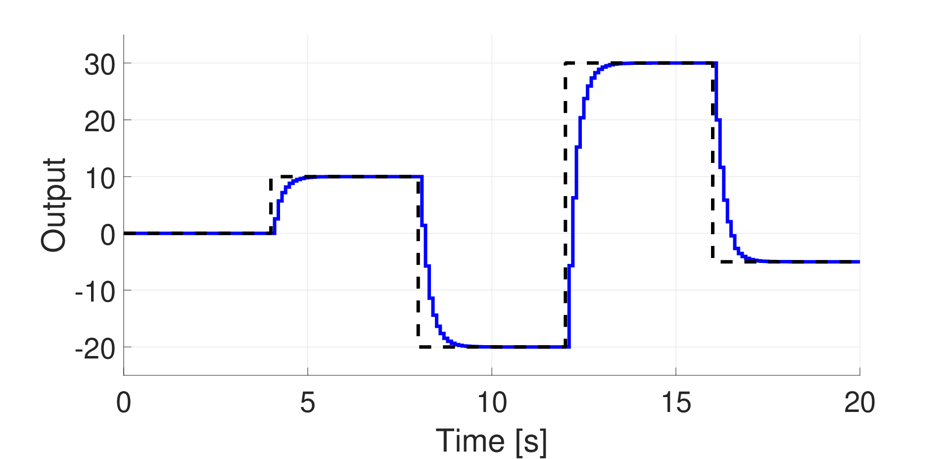
Fig. 4: Output trajectory of the closed-loop discrete-time system with state-feedback and explicit integral action. Black dashed line: reference signal trajectory; blue line: output signal trajectory.

In Figure 4 the reference tracking results of the closed-loop system are depicted, where we can see that the closed-loop system enjoys δ\deltaISS and its equilibria are asymptotically stable even if the open-loop system displays unstable dynamics, as we can see from the second (linear) state equation of the open-loop system. Furthermore, due to the explicit integral action, a zero steady-state error is also achieved.

On the other hand, if we take f2​(⋅)=tanh⁡(⋅)f_{2}(\cdot)=\tanh(\cdot), matrix PP is constrained to have the following structure, on the basis of Theorem 2: P=diag​(p1,p2,p3)P=\text{diag}(p_{1},p_{2},p_{3}), where p1,p2,p3∈ℝp_{1},p_{2},p_{3}\in\mathbb{R}. An unfeasible solution is returned by solving (24) (where W=I3W=I_{3}), corroborating the statement in Proposition 15.

If the control schemes in Figure 3 cannot be used to achieve zero steady-state error while ensuring δ\deltaISS for the closed-loop system, a possible solution to improve the static performance could be the use of a δ\deltaISS feedforward compensator in the class (4). Since it is dynamic, this compensator can be used to enhance both static and dynamic performances. Moreover, provided that the closed-loop system is δ\deltaISS, the addition of a δ\deltaISS feedforward compensator preserves the δ\deltaISS of the overall control system. This fact follows straightforwardly from the result in Proposition 9, since such a component is placed in series to the closed-loop system. Future research will address methods for the design of feedforward compensators, as well as the analysis of the dynamic performances of the control system.

V Simulation results

In order to validate the theoretical results in the previous sections we propose here a simulation example. The case study consists of the control of the following ESN-based nonlinear SISO system with ns=8n_{s}=8 states

xs​(k+1)\displaystyle x_{s}(k+1) =ζs​(Wxs​xs​(k)+Wus​us​(k)+Wys​ys​(k)),\displaystyle\!=\!\zeta_{s}(W_{x_{s}}x_{s}(k)+W_{u_{s}}u_{s}(k)+W_{y_{s}}y_{s}(k))\,, (35a)
ys​(k)\displaystyle y_{s}(k) =Wo​u​t1s​xs​(k),\displaystyle\!=\!W_{out_{1_{s}}}x_{s}(k)\,, (35b)

where the direct dependence of the input in the output equation is absent, i.e., Wo​u​t2s=0W_{out_{2_{s}}}=0, and ζsi​(⋅)=i​d​(⋅)\zeta_{s_{i}}(\cdot)=id(\cdot) for i=1,…,5i=1,\dots,5, whereas ζsi​(⋅)=tanh⁡(⋅)\zeta_{s_{i}}(\cdot)=\tanh(\cdot) for i=6,7,8i=6,7,8. The structure of the state equations, both nonlinear and linear, is such that the output can take unbounded values, paving the way to the possible inclusion of an explicit integral action (according to Proposition 15), and to more freedom in the control design (e.g., see Theorem 2).

The model (35) is identified using a noiseless dataset containing 7000070000 normalized input-output data collected with a sampling time Ts=25​sT_{s}=25\ s from a simulated pH neutralization process (see [19, 27, 28] for a detailed description of the system model). The pH process is a nonlinear SISO dynamical system where the input is the alkaline flowrate, and the output is the pH concentration. The training input data consist of a multilevel pseudo-random signal (MPRS) [27], whose amplitude is in the range [12,16]​m​L/s[12,16]\ mL/s. The training is carried out according to the “ESN training algorithm” (see [19] for an accurate description). Basically, WxsW_{x_{s}}, WusW_{u_{s}}, and WysW_{y_{s}} are randomly generated, whereas Wo​u​t1sW_{out_{1_{s}}} is obtained by solving a least squares problem based on the available dataset, where the initial 500500 data points are discarded to accommodate the effect of the initial transient. To test the identification performance, the following fitting index is calculated over a validation dataset composed of 3000030000 new normalized input-output data

FIT%=100⋅(1−‖y→−y→s‖‖y→−y¯‖)∈(−∞,100],FIT_{\%}=100\cdot\left(1-\frac{\|\vec{y}-\vec{y}_{s}\|}{\|\vec{y}-\bar{y}\|}\right)\in(-\infty,100]\,, (36)

where y→\vec{y} is the real system output sequence, y→s\vec{y}_{s} is the output sequence obtained with (35) and y¯\bar{y} is a vector with all the elements equal to the mean value of the real output sequence y→\vec{y}. A satisfactory fitting FIT%=84.1452%FIT_{\%}=84.1452\% is achieved.

Refer to caption
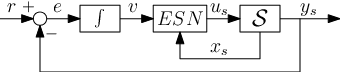
Fig. 5: Control scheme with explicit integral action and ESN in series: ∫\int is the discrete-time integrator, E​S​NESN the echo state dynamic controller, and 𝒮\mathcal{S} the system to be controlled.

The control objective in this example is the achievement of perfect asymptotic tracking of constant reference signals. To this aim, the control architecture in Figure 5 is taken into account, where an explicit integral action is also embedded. In particular, 𝒮\mathcal{S} is the system (35) to be controlled, whose state is assumed measurable, “∫\int” is defined as in (33) by setting M=1M=1, and “E​S​NESN” is a non-strictly proper ESN controller with nc=5n_{c}=5 states, whose input vector contains the integrator output v⁡(k)v(k) jointly to the system state vector xs​(k)x_{s}(k). Overall, the controller equations are the following

xc​(k+1)\displaystyle x_{c}(k+1) =ζc​(Wxc​xc​(k)+Wuc​uc​(k)+Wyc​yc​(k)),\displaystyle=\zeta_{c}(W_{x_{c}}x_{c}(k)+W_{u_{c}}u_{c}(k)+W_{y_{c}}y_{c}(k))\,, (37a)
η⁡(k+1)\displaystyle\eta(k+1) =η⁡(k)+e⁡(k),\displaystyle=\eta(k)+e(k)\,, (37b)
yc​(k)\displaystyle y_{c}(k) =Wo​u​t1c​xc​(k)+Wo​u​t2c​uc​(k),\displaystyle=W_{out_{1_{c}}}x_{c}(k)+W_{out_{2_{c}}}u_{c}(k)\,, (37c)

where ζci​(⋅)=tanh⁡(⋅)\zeta_{c_{i}}(\cdot)=\tanh(\cdot) for all i=1,…,5i=1,\dots,5, uc​(k)=[v⁡(k)xs​(k)T]Tu_{c}(k)=\begin{bmatrix}v(k)&x_{s}(k)^{T}\end{bmatrix}^{T}, and v⁡(k)=η⁡(k)+e⁡(k)v(k)=\eta(k)+e(k). Let us define Wuc=[Wuc​vWuc​x]W_{u_{c}}=\begin{bmatrix}W_{u_{cv}}&W_{u_{cx}}\end{bmatrix}, and Wo​u​t2c=[Wo​u​t2c​vWo​u​t2c​x]W_{out_{2_{c}}}=\begin{bmatrix}W_{out_{2_{cv}}}&W_{out_{2_{cx}}}\end{bmatrix}, where Wuc​v∈ℝncW_{u_{cv}}\in\mathbb{R}^{n_{c}}, Wuc​x∈ℝnc×nsW_{u_{cx}}\in\mathbb{R}^{n_{c}\times n_{s}}, Wo​u​t2c​v∈ℝW_{out_{2_{cv}}}\in\mathbb{R}, and Wo​u​t2c​x∈ℝ1×nsW_{out_{2_{cx}}}\in\mathbb{R}^{1\times n_{s}}. Also, let us introduce x⁡(k)=[xc​(k)Tη⁡(k)xs​(k)T]Tx(k)=\begin{bmatrix}x_{c}(k)^{T}&\eta(k)&x_{s}(k)^{T}\end{bmatrix}^{T}, and f⁡(⋅)=[ζc​(⋅)Ti​d​(⋅)ζs​(⋅)T]Tf(\cdot)=\begin{bmatrix}\zeta_{c}(\cdot)^{T}&id(\cdot)&\zeta_{s}(\cdot)^{T}\end{bmatrix}^{T}. By recalling that us​(k)=yc​(k)u_{s}(k)=y_{c}(k) and e⁡(k)=r⁡(k)−ys​(k)e(k)=r(k)-y_{s}(k), we can write the closed-loop system equations in the class (4), where the matrix AA is defined as

A=[Wxc+Wyc​Wo​u​t1cWuc​v+Wyc​Wo​u​t2c​vA1301,nc1−Wo​u​t1sWus​Wo​u​t1cWus​Wo​u​t2c​vA33],\displaystyle A=\left[\begin{matrix}W_{x_{c}}+W_{y_{c}}W_{out_{1_{c}}}&W_{u_{cv}}+W_{y_{c}}W_{out_{2_{cv}}}&A_{13}\\ 0_{1,n_{c}}&1&-W_{out_{1_{s}}}\\ W_{u_{s}}W_{out_{1_{c}}}&W_{u_{s}}W_{out_{2_{cv}}}&A_{33}\end{matrix}\right]\,,

where A13=Wuc​x−Wuc​v​Wo​u​t1s+Wyc​(Wo​u​t2c​x−Wo​u​t2c​v​Wo​u​t1s)A_{13}=W_{u_{cx}}-W_{u_{cv}}W_{out_{1_{s}}}+W_{y_{c}}(W_{out_{2_{cx}}}-W_{out_{2_{cv}}}W_{out_{1_{s}}}), and A33=Wxs+Wys​Wo​u​t1s+Wus​(Wo​u​t2c​x−Wo​u​t2c​v​Wo​u​t1s)A_{33}=W_{x_{s}}+W_{y_{s}}W_{out_{1_{s}}}+W_{u_{s}}(W_{out_{2_{cx}}}-W_{out_{2_{cv}}}W_{out_{1_{s}}}). Since WxcW_{x_{c}}, WucW_{u_{c}}, and WycW_{y_{c}} are known randomly generated matrices, we can rewrite AA as F+G​JF+GJ, where

F=[WxcWuc​vWuc​x−Wuc​v​Wo​u​t1s01,nc1−Wo​u​t1s0ns,nc0ns,1Wxs+Wys​Wo​u​t1s],G=[Wyc0Wus],\displaystyle F=\left[\begin{matrix}W_{x_{c}}&W_{u_{cv}}&W_{u_{cx}}-W_{u_{cv}}W_{out_{1_{s}}}\\ 0_{1,n_{c}}&1&-W_{out_{1_{s}}}\\ 0_{n_{s},n_{c}}&0_{n_{s},1}&W_{x_{s}}+W_{y_{s}}W_{out_{1_{s}}}\end{matrix}\right]\,,\ \ G=\left[\begin{matrix}W_{y_{c}}\\ 0\\ W_{u_{s}}\end{matrix}\right]\,,

and J=[Wo​u​t1cWo​u​t2c​vWo​u​t2c​x−Wo​u​t2c​v​Wo​u​t1s]J\!=\!\begin{bmatrix}W_{out_{1_{c}}}&W_{out_{2_{cv}}}&W_{out_{2_{cx}}}\!-\!W_{out_{2_{cv}}}\!W_{out_{1_{s}}}\end{bmatrix} takes the role of the control gain. Note that the unknown controller parameters can be computed as [Wo​u​t1cWo​u​t2c]=J​E−1\begin{bmatrix}W_{out_{1_{c}}}&W_{out_{2_{c}}}\end{bmatrix}=JE^{-1}, where

E=[Inc0nc,10nc,ns01,nc1−Wo​u​t1s0ns,nc0ns,1Ins].E=\begin{bmatrix}I_{n_{c}}&0_{n_{c},1}&0_{n_{c},n_{s}}\\ 0_{1,n_{c}}&1&-W_{out_{1_{s}}}\\ 0_{n_{s},n_{c}}&0_{n_{s},1}&I_{n_{s}}\end{bmatrix}\,.

According to Proposition 11, the matrix PP must have the following block diagonal structure: P=diag​(PD1,PF,PD2)P=\text{diag}(P_{D_{1}},P_{F},P_{D_{2}}), where PD1∈ℝ5×5P_{D_{1}}\in\mathbb{R}^{5\times 5} and PD2∈ℝ3×3P_{D_{2}}\in\mathbb{R}^{3\times 3} are diagonal matrices, whereas PF∈ℝ6×6P_{F}\in\mathbb{R}^{6\times 6} is a full symmetric matrix. A feasible solution is returned by solving (24), where W=Inc+ns+1W=I_{n_{c}+n_{s}+1}, with YALMIP and MOSEK [25, 26], ensuring that the closed-loop system enjoys the δ\deltaISS property due to Proposition 11.

Refer to caption
Fig. 6: Denormalized output trajectories of the closed-loop discrete-time system starting from different initial conditions. Black dashed line: reference trajectory; colored lines: output trajectories for 2020 different initial conditions.

In Figure 6 the reference tracking results of the closed-loop system starting from 2020 different random initial conditions are depicted, where we can see that the equilibria are asymptotically stable and the output trajectories converge to each other in view of the δ\deltaISS property. Moreover, due to the explicit integral action, a zero steady-state error is achieved.

The previously tuned controller is also tested on the pH process physics-based simulator. To this aim, some remarks are due. Firstly, in the control scheme, a denormalization of the control variable usu_{s} and a normalization of the output ysy_{s} are performed upstream and downstream of the process, respectively. A normalization of the reference signal is also carried out. The same normalization parameters applied in the identification are employed.

The second issue to be considered concerns the fact that the state measurements of the system (35), necessary for the state-feedback, are not available in this second case. Hence, a suitable observer is required. As suggested in Section IV-B, the following observer is tuned:

x^s​(k+1)\displaystyle\hat{x}_{s}(k+1) =ζs​((Wxs+Wys​Wo​u​t1s)​x^s​(k)+Wus​us​(k)+L⁡(ys​(k)−y^s​(k))),\displaystyle=\zeta_{s}((W_{x_{s}}+W_{y_{s}}W_{out_{1_{s}}})\hat{x}_{s}(k)+W_{u_{s}}u_{s}(k)+L(y_{s}(k)-\hat{y}_{s}(k)))\,, (38a)
y^s​(k)\displaystyle\hat{y}_{s}(k) =Wo​u​t1s​x^s​(k),\displaystyle=W_{out_{1_{s}}}\hat{x}_{s}(k)\,, (38b)

where the observer gain LL is designed using the result in Proposition 13.

Refer to caption
Fig. 7: Output trajectories of the closed-loop system using the simulated pH process and starting from different initial conditions. Black dashed line: reference trajectory; colored lines: output trajectories for 2020 different initial conditions.

In Figure 7 the reference tracking results of the closed-loop system using the simulated pH process and starting from 2020 different random initial conditions are represented, where we can see that the equilibria are asymptotically stable and, due to the explicit integral action, a zero steady-state error is also achieved.

VI Conclusions

In this paper, a δ\deltaISS condition for a generic class of RNNs has been proposed. The reduced conservativeness of this condition with respect to other conditions in the literature has been proven. Moreover, the use of this condition for control design purposes has been widely investigated. Simulation results have corroborated the effectiveness of the theoretical results.
Future work will first tackle a number of issues remained open in this work. Firstly, a possible extension to alternative conditions to the one in Theorem 2 in order to include other classes of RNNs (e.g., multi-layers NNARX or long short-term memory networks) will be addressed. Secondly, the development of a (possibly data-based) cost function which takes into account the desired dynamic performances of the control system will be investigated. Then, we will address the design of a suitable δ\deltaISS feedforward compensator to be used to achieve static precision in case an explicit integral action cannot be embedded in the control scheme. Furthermore, the convergence rate of the observer together with the analysis of the case in which a non-measurable disturbance acts on the system will be studied. Finally, the application of the theoretical results in this paper to an experimental apparatus will be carried out.

Appendix

Proof of Proposition 3.

Firstly, note that the condition ‖Wx∗‖<1\|W_{x}^{*}\|<1 is equivalent to the condition

Wx∗T​In​Wx∗−In≺0.\displaystyle{W_{x}^{*}}^{T}I_{n}W_{x}^{*}-I_{n}\prec 0. (39)

Also note that, since Lp≤1L_{p}\leq 1, we can set W=InW=I_{n}. Then, for ESNs, Theorem 2 states that system (5) in the state-space form (4) is δ\deltaISS if ∃P=PT=diag​(P1,P2)≻0\exists P=P^{T}=\text{diag}(P_{1},P_{2})\succ 0, where P1∈ℝν×νP_{1}\in\mathbb{R}^{\nu\times\nu} is diagonal and P2∈ℝm×mP_{2}\in\mathbb{R}^{m\times m} is full, such that

AT​P​A−P=[Wx∗T​P1​Wx∗−P1Wx∗T​P1​Wy​Wo​u​t2Wo​u​t2T​WyT​P1​Wx∗Wo​u​t2T​WyT​P1​Wy​Wo​u​t2−P2]≺0,\displaystyle\begin{split}A^{T}PA-P=\left[\begin{matrix}W_{x}^{*T}P_{1}W_{x}^{*}-P_{1}&W_{x}^{*T}P_{1}W_{y}W_{out_{2}}\\ W_{out_{2}}^{T}W_{y}^{T}P_{1}W_{x}^{*}&W_{out_{2}}^{T}W_{y}^{T}P_{1}W_{y}W_{out_{2}}-P_{2}\end{matrix}\right]\prec 0\,,\end{split}

where AA is defined as in (6).
We define a generic vector v=[v1Tv2T]Tv=\begin{bmatrix}v_{1}^{T}&v_{2}^{T}\end{bmatrix}^{T}, where v1∈ℝνv_{1}\in\mathbb{R}^{\nu} and v2∈ℝmv_{2}\in\mathbb{R}^{m}. Therefore, we want to prove that vT​(AT​P​A−P)​v<0v^{T}(A^{T}PA-P)v<0 for any v≠0n,1v\neq 0_{n,1}. Hence, vT​(AT​P​A−P)​v=v1T​(Wx∗T​P1​Wx∗−P1)​v1+2​v2T​Wo​u​t2T​WyT​P1​Wx∗​v1+v2T​(Wo​u​t2T​WyT​P1​Wy​Wo​u​t2−P2)​v2v^{T}(A^{T}PA-P)v=v_{1}^{T}(W_{x}^{*T}P_{1}W_{x}^{*}-P_{1})v_{1}+2v_{2}^{T}W_{out_{2}}^{T}W_{y}^{T}P_{1}W_{x}^{*}v_{1}+v_{2}^{T}(W_{out_{2}}^{T}W_{y}^{T}P_{1}W_{y}W_{out_{2}}-P_{2})v_{2}. Furthermore, in view of Property 1, for any τ≠0\tau\neq 0,

vT​(AT​P​A−P)​v≤v1T​((1+τ2)​Wx∗T​P1​Wx∗−P1)​v1+v2T​((1+1τ2)​Wo​u​t2T​WyT​P1​Wy​Wo​u​t2−P2)​v2.\displaystyle v^{T}(A^{T}PA-P)v\leq v_{1}^{T}((1+\tau^{2})W_{x}^{*T}P_{1}W_{x}^{*}-P_{1})v_{1}+v_{2}^{T}((1+\frac{1}{\tau^{2}})W_{out_{2}}^{T}W_{y}^{T}P_{1}W_{y}W_{out_{2}}-P_{2})v_{2}\,.

Now, by setting P1=InP_{1}=I_{n}, it follows from (39) that (1+τ2)​Wx∗T​P1​Wx∗−P1≺0(1+\tau^{2})W_{x}^{*T}P_{1}W_{x}^{*}-P_{1}\prec 0 for a sufficiently small τ\tau. Moreover, note that Aτ∗=(1+1τ2)​Wo​u​t2T​WyT​P1​Wy​Wo​u​t2⪯λm​a​x​(Aτ∗)​ImA_{\tau}^{*}=(1+\frac{1}{\tau^{2}})W_{out_{2}}^{T}W_{y}^{T}P_{1}W_{y}W_{out_{2}}\preceq\lambda_{max}(A_{\tau}^{*})I_{m}, where λm​a​x​(Aτ∗)≥0\lambda_{max}(A_{\tau}^{*})\geq 0. By setting P2=λp​ImP_{2}=\lambda_{p}I_{m}, with λp>λm​a​x​(Aτ∗)\lambda_{p}>\lambda_{max}(A_{\tau}^{*}), we have that (1+1τ2)​Wo​u​t2T​WyT​P1​Wy​Wo​u​t2−P2≺0(1+\frac{1}{\tau^{2}})W_{out_{2}}^{T}W_{y}^{T}P_{1}W_{y}W_{out_{2}}-P_{2}\prec 0. This implies that vT​(AT​P​A−P)​v<0v^{T}(A^{T}PA-P)v<0 for any v≠0n,1v\neq 0_{n,1}, and the statement follows. ∎

Proof of Proposition 5.

The objective is to prove that the fulfilment of the assumption of Proposition 4 implies the fulfilment of the assumptions of Theorem 2. The latter, for a 1-layer NNARX, require the existence of a matrix P=PT≻0P=P^{T}\succ 0 such that

A~T​P​A~−P≺0,\widetilde{A}^{T}P\widetilde{A}-P\prec 0\,,

where A~=W​A\widetilde{A}=WA, A=[0τ,l+m~Iτ0τ,ν0l,l+m~0l,τW00m~,l+m~0m~,τ0m~,νWϕ1Wϕ2Wϕ3​W0]A=\left[\begin{matrix}0_{\tau,l+\widetilde{m}}&I_{\tau}&0_{\tau,\nu}\\ 0_{l,l+\widetilde{m}}&0_{l,\tau}&W_{0}\\ 0_{\widetilde{m},l+\widetilde{m}}&0_{\widetilde{m},\tau}&0_{\widetilde{m},\nu}\\ W_{\phi_{1}}&W_{\phi_{2}}&W_{\phi_{3}}W_{0}\end{matrix}\right], W=[In−ν0n−ν,ν0ν,n−νLp​Iν],P=[P~0n−ν,ν0ν,n−νPD],W=\left[\begin{matrix}I_{n-\nu}&0_{n-\nu,\nu}\\ 0_{\nu,n-\nu}&L_{p}I_{\nu}\\ \end{matrix}\right],\ P=\left[\begin{matrix}\widetilde{P}&0_{n-\nu,\nu}\\ 0_{\nu,n-\nu}&P_{D}\\ \end{matrix}\right], P~∈ℝ(n−ν)×(n−ν)\widetilde{P}\in\mathbb{R}^{(n-\nu)\times(n-\nu)}, and PD∈ℝν×νP_{D}\in\mathbb{R}^{\nu\times\nu} is a diagonal matrix. For notational clarity, we recall that n−ν=τ+l+m~n-\nu=\tau+l+\widetilde{m}. Moreover, we can write A=Aϕ​W~0A=A_{\phi}\widetilde{W}_{0}, by defining

Aϕ=[0τ,l+m~Iτ0τ,l0l,l+m~0l,τIl0m~,l+m~0m~,τ0m~,lWϕ1Wϕ2Wϕ3],A_{\phi}=\left[\begin{matrix}0_{\tau,l+\widetilde{m}}&I_{\tau}&0_{\tau,l}\\ 0_{l,l+\widetilde{m}}&0_{l,\tau}&I_{l}\\ 0_{\widetilde{m},l+\widetilde{m}}&0_{\widetilde{m},\tau}&0_{\widetilde{m},l}\\ W_{\phi_{1}}&W_{\phi_{2}}&W_{\phi_{3}}\end{matrix}\right]\,,

and

W~0=[Il+m~0l+m~,τ0l+m~,ν0τ,l+m~Iτ0τ,ν0l,l+m~0l,τW0].\widetilde{W}_{0}=\left[\begin{matrix}I_{l+\widetilde{m}}&0_{l+\widetilde{m},\tau}&0_{l+\widetilde{m},\nu}\\ 0_{\tau,l+\widetilde{m}}&I_{\tau}&0_{\tau,\nu}\\ 0_{l,l+\widetilde{m}}&0_{l,\tau}&W_{0}\end{matrix}\right]\,.

Furthermore, we can define A~ϕ=W​Aϕ=[QLp​Wϕ]\widetilde{A}_{\phi}=WA_{\phi}=\left[\begin{matrix}Q\\ L_{p}W_{\phi}\end{matrix}\right], where Wϕ=[Wϕ1Wϕ2Wϕ3],W_{\phi}=\begin{bmatrix}W_{\phi_{1}}&W_{\phi_{2}}&W_{\phi_{3}}\end{bmatrix}\,, and

Q=[0τ,l+m~Iτ0τ,l0l,l+m~0l,τIl0m~,l+m~0m~,τ0m~,l].Q=\left[\begin{matrix}0_{\tau,l+\widetilde{m}}&I_{\tau}&0_{\tau,l}\\ 0_{l,l+\widetilde{m}}&0_{l,\tau}&I_{l}\\ 0_{\widetilde{m},l+\widetilde{m}}&0_{\widetilde{m},\tau}&0_{\widetilde{m},l}\end{matrix}\right]\,.

Therefore, the assumptions of Theorem 2 can be rewritten as follows

W~0T​A~ϕT​P​A~ϕ​W~0−P\displaystyle\widetilde{W}_{0}^{T}\widetilde{A}_{\phi}^{T}P\widetilde{A}_{\phi}\widetilde{W}_{0}-P ≺0,\displaystyle\prec 0\,,
W~0T​(QT​P~​Q+Lp2​WϕT​PD​Wϕ)​W~0−P\displaystyle\widetilde{W}_{0}^{T}(Q^{T}\widetilde{P}Q+L_{p}^{2}W_{\phi}^{T}P_{D}W_{\phi})\widetilde{W}_{0}-P ≺0,\displaystyle\prec 0\,,
W~0T​QT​P~​Q​W~0−P+Lp2​W~0T​WϕT​PD​Wϕ​W~0\displaystyle\widetilde{W}_{0}^{T}Q^{T}\widetilde{P}Q\widetilde{W}_{0}-P+L_{p}^{2}\widetilde{W}_{0}^{T}W_{\phi}^{T}P_{D}W_{\phi}\widetilde{W}_{0} ≺0.\displaystyle\prec 0\,. (40)

Now, let us choose a block diagonal P~\widetilde{P}, i.e., P~=P~T=diag​(P~1,P~2,P~3)\widetilde{P}=\widetilde{P}^{T}=\text{diag}(\widetilde{P}_{1},\widetilde{P}_{2},\widetilde{P}_{3}), where P~1∈ℝτ×τ\widetilde{P}_{1}\in\mathbb{R}^{\tau\times\tau}, P~2∈ℝl×l\widetilde{P}_{2}\in\mathbb{R}^{l\times l}, and P~3∈ℝm~×m~\widetilde{P}_{3}\in\mathbb{R}^{\widetilde{m}\times\widetilde{m}}. With this choice, we can compute

W~0T​QT​P~​Q​W~0=W~0T​[0l+m~,l+m~0l+m~,τ0l+m~,l0τ,l+m~P~10τ,l0l,l+m~0l,τP~2]​W~0=[P~00n−ν,ν0ν,n−νW0T​P~2​W0],\displaystyle\widetilde{W}_{0}^{T}Q^{T}\widetilde{P}Q\widetilde{W}_{0}=\widetilde{W}_{0}^{T}\left[\begin{matrix}0_{l+\widetilde{m},l+\widetilde{m}}&0_{l+\widetilde{m},\tau}&0_{l+\widetilde{m},l}\\ 0_{\tau,l+\widetilde{m}}&\widetilde{P}_{1}&0_{\tau,l}\\ 0_{l,l+\widetilde{m}}&0_{l,\tau}&\widetilde{P}_{2}\end{matrix}\right]\widetilde{W}_{0}=\left[\begin{matrix}\widetilde{P}_{0}&0_{n-\nu,\nu}\\ 0_{\nu,n-\nu}&W_{0}^{T}\widetilde{P}_{2}W_{0}\end{matrix}\right]\,,

where P~0=[0l+m~,l+m~0l+m~,τ0τ,l+m~P~1]\widetilde{P}_{0}=\left[\begin{matrix}0_{l+\widetilde{m},l+\widetilde{m}}&0_{l+\widetilde{m},\tau}\\ 0_{\tau,l+\widetilde{m}}&\widetilde{P}_{1}\\ \end{matrix}\right]. Thus, we have that

W~0T​QT​P~​Q​W~0−P=[P~0−P~0n−ν,ν0ν,n−νW0T​P~2​W0−PD].\displaystyle\widetilde{W}_{0}^{T}Q^{T}\widetilde{P}Q\widetilde{W}_{0}-P=\left[\begin{matrix}\widetilde{P}_{0}-\widetilde{P}&0_{n-\nu,\nu}\\ 0_{\nu,n-\nu}&W_{0}^{T}\widetilde{P}_{2}W_{0}-P_{D}\end{matrix}\right]\,.

Then, let us choose

P~1=α⋅diag​(Il+m~,2​Il+m~,…,(N−2)​Il+m~,(N−1)​Im~),\widetilde{P}_{1}=\alpha\cdot\text{diag}(I_{l+\widetilde{m}},2I_{l+\widetilde{m}},\dots,(N-2)I_{l+\widetilde{m}},(N-1)I_{\widetilde{m}})\,,

P~2=α⁡(N−1)​Il\widetilde{P}_{2}=\alpha(N-1)I_{l}, P~3=α​N​Im~\widetilde{P}_{3}=\alpha NI_{\widetilde{m}}, for any scalar α>0\alpha>0, and PD=β​IνP_{D}=\beta I_{\nu}, for any scalar β>0\beta>0. Hence, according to the previous choices, we can rewrite (40) as

[−α​In−ν0n−ν,ν0ν,n−να⁡(N−1)​W0T​W0−β​Iν]+β​Lp2​W~0T​WϕT​Wϕ​W~0≺0.\displaystyle\left[\begin{matrix}-\alpha I_{n-\nu}&0_{n-\nu,\nu}\\ 0_{\nu,n-\nu}&\alpha(N-1)W_{0}^{T}W_{0}-\beta I_{\nu}\end{matrix}\right]+\beta L_{p}^{2}\widetilde{W}_{0}^{T}W_{\phi}^{T}W_{\phi}\widetilde{W}_{0}\prec 0\,.

By adding and subtracting γ​W~0T​W~0\gamma\widetilde{W}_{0}^{T}\widetilde{W}_{0}, for any scalar γ>0\gamma>0, the condition (40) becomes

[−α​In−ν0n−ν,ν0ν,n−να⁡(N−1)​W0T​W0−β​Iν]+γ​W~0T​W~0+W~0T​(β​Lp2​WϕT​Wϕ−γ​I(l+m~)​N)​W~0≺0.\displaystyle\left[\begin{matrix}-\alpha I_{n-\nu}&0_{n-\nu,\nu}\\ 0_{\nu,n-\nu}&\alpha(N-1)W_{0}^{T}W_{0}-\beta I_{\nu}\end{matrix}\right]+\gamma\widetilde{W}_{0}^{T}\widetilde{W}_{0}+\widetilde{W}_{0}^{T}(\beta L_{p}^{2}W_{\phi}^{T}W_{\phi}-\gamma I_{(l+\widetilde{m})N})\widetilde{W}_{0}\prec 0\,. (41)

Now, note that if both

[(γ−α)​In−ν0n−ν,ν0ν,n−ν(α⁡(N−1)+γ)​W0T​W0−β​Iν]\displaystyle\left[\begin{matrix}(\gamma-\alpha)I_{n-\nu}&0_{n-\nu,\nu}\\ 0_{\nu,n-\nu}&(\alpha(N-1)+\gamma)W_{0}^{T}W_{0}-\beta I_{\nu}\end{matrix}\right] ≺0\displaystyle\prec 0 (42)
β​Lp2​WϕT​Wϕ−γ​I(l+m~)​N\displaystyle\beta L_{p}^{2}W_{\phi}^{T}W_{\phi}-\gamma I_{(l+\widetilde{m})N} ≺0\displaystyle\prec 0 (43)

are fulfilled, then (41) certainly holds. Therefore, we want to prove that there exist α>0\alpha>0, β>0\beta>0, and γ>0\gamma>0 such that (42) and (43) hold provided that the assumption of Proposition 4 is fulfilled. Firstly, note that (42) holds if and only if

γ\displaystyle\gamma <α,\displaystyle<\alpha\,, (44)
‖W0‖2=λm​a​x​(W0T​W0)\displaystyle\|W_{0}\|^{2}=\lambda_{max}(W_{0}^{T}W_{0}) <βα⁡(N−1)+γ.\displaystyle<\frac{\beta}{\alpha(N-1)+\gamma}\,. (45)

Secondly, (43) holds if and only if

‖Wϕ‖2=λm​a​x​(WϕT​Wϕ)\displaystyle\|W_{\phi}\|^{2}=\lambda_{max}(W_{\phi}^{T}W_{\phi}) <γβ​Lp2.\displaystyle<\frac{\gamma}{\beta L_{p}^{2}}\,. (46)

Furthermore, if (44) holds, we have that (45) is certainly fulfilled if

‖W0‖2\displaystyle\|W_{0}\|^{2} <βα​N\displaystyle<\frac{\beta}{\alpha N} (47)

holds. Hence, if conditions (44), (46), and (47) are satisfied, we have that (41) holds, implying the fulfilment of the assumptions of Theorem 2. Finally, to have (44), (46), and (47) fulfilled, we have to prove the existence of positive α\alpha, β\beta, and γ\gamma such that

‖Wϕ‖2​Lp2<γβ<αβ<1‖W0‖2​N.\displaystyle\|W_{\phi}\|^{2}L_{p}^{2}<\frac{\gamma}{\beta}<\frac{\alpha}{\beta}<\frac{1}{\|W_{0}\|^{2}N}\,. (48)

In particular, in view of the assumption of Proposition 4, i.e., ‖W0‖​‖Wϕ‖<1Lp​N\|W_{0}\|\|W_{\phi}\|<\frac{1}{L_{p}\sqrt{N}}, it follows that ‖Wϕ‖2​Lp2<1‖W0‖2​N\|W_{\phi}\|^{2}L_{p}^{2}<\frac{1}{\|W_{0}\|^{2}N}. Thus, it is always possible to find positive real numbers α\alpha, β\beta, and γ\gamma such that (48) holds thanks to the completeness axiom of real numbers. This concludes the proof. ∎

Proof of Proposition 7.

Firstly, if E=0n,nE=0_{n,n} and oi=1o_{i}=1 ∀i∈ℒ\forall i\in\mathcal{L}, we have that M^=W​|A|\hat{M}=W|A|, where A=O​A^A=O\hat{A}. Accordingly, the assumption of Proposition 6 requires the existence of a matrix P=PT≻0P=P^{T}\succ 0 such that

|A|T​WT​P​W​|A|−P≺0.\displaystyle|A|^{T}\,W^{T}P\,W\,|A|\,-\,P\prec 0\,. (49)

This condition represents also the stability condition for

x~​(k+1)=W​|A|​x~​(k),\displaystyle\tilde{x}(k+1)=W\,|A|\,\tilde{x}(k)\,, (50)

which is a discrete-time linear positive system. Hence, as stated in [29, Theorem 15], system (50) is asymptotically stable if and only if there exists a diagonal P≻0P\succ 0 fulfilling condition (49).

Therefore, let us consider a matrix P=diag​(p1,…,pn)∈ℝn×nP=\text{diag}(p_{1},\dots,p_{n})\in\mathbb{R}^{n\times n}, with pi>0p_{i}>0. For any generic vector v∈ℝnv\in\mathbb{R}^{n}, v≠0n,1v\neq 0_{n,1}, condition (49) implies that

vT​(|A|T​WT​P​W​|A|−P)​v<0,\displaystyle v^{T}(|A|^{T}\,W^{T}P\,W\,|A|\,-\,P)\,v<0\,,

which becomes

(i)∑j=1npj​Lp​j2​(∑i=1n|aj​i|​vi)2−∑j=1npj​vj2<0.\displaystyle(i)\qquad\sum_{j=1}^{n}p_{j}L_{pj}^{2}\bigg(\sum_{i=1}^{n}|a_{ji}|v_{i}\bigg)^{2}\;-\;\sum_{j=1}^{n}p_{j}v_{j}^{2}<0\,.

On the other hand, following the same reasoning, for all v~∈ℝn\tilde{v}\in\mathbb{R}^{n}, v~≠0n,1\tilde{v}\neq 0_{n,1}, condition (13) in Theorem 2 with a diagonal PP is equivalent to

(i​i)∑j=1npj​Lp​j2​(∑i=1naj​i​v~i)2−∑j=1npj​v~j2<0.\displaystyle(ii)\qquad\sum_{j=1}^{n}p_{j}L_{pj}^{2}\bigg(\sum_{i=1}^{n}a_{ji}\tilde{v}_{i}\bigg)^{2}\;-\;\sum_{j=1}^{n}p_{j}\tilde{v}_{j}^{2}<0\,.

We want to show now that, if (i)(i) holds for any v∈ℝnv\in\mathbb{R}^{n}, v≠0n,1v\neq 0_{n,1}, it follows that (i​i)(ii) holds for any v~∈ℝn\tilde{v}\in\mathbb{R}^{n}, v~≠0n,1\tilde{v}\neq 0_{n,1}.

Let us consider a generic v~∈ℝn\tilde{v}\in\mathbb{R}^{n}, v~≠0n,1\tilde{v}\neq 0_{n,1}. It follows that v=|v~|v=|\tilde{v}| satisfies (i)(i) by assumption. Also, note that

|∑i=1naj​i​v~i|≤∑i=1n|aj​i​v~i|=∑i=1n|aj​i|​|v~i|=∑i=1n|aj​i|​vi,\displaystyle\bigg|\sum_{i=1}^{n}a_{ji}\,\tilde{v}_{i}\bigg|\leq\sum_{i=1}^{n}\Big|a_{ji}\,\tilde{v}_{i}\Big|=\sum_{i=1}^{n}|a_{ji}|\,|\tilde{v}_{i}|\,=\sum_{i=1}^{n}|a_{ji}|\,v_{i}\,,

which implies that

∑j=1npj​Lp​j2​(∑i=1naj​i​v~i)2≤∑j=1npj​Lp​j2​(∑i=1n|aj​i|​vi)2.\displaystyle\sum_{j=1}^{n}p_{j}L_{pj}^{2}\bigg(\sum_{i=1}^{n}a_{ji}\,\tilde{v}_{i}\bigg)^{2}\leq\;\,\sum_{j=1}^{n}p_{j}L_{pj}^{2}\bigg(\sum_{i=1}^{n}|a_{ji}|\,v_{i}\bigg)^{2}\,. (51)

Moreover, note that

∑j=1npj​v~j2=∑j=1npj​|v~j|2=∑j=1npj​vj2.\displaystyle\sum_{j=1}^{n}p_{j}\tilde{v}_{j}^{2}\,=\sum_{j=1}^{n}p_{j}|\tilde{v}_{j}|^{2}\,=\sum_{j=1}^{n}p_{j}v_{j}^{2}\,. (52)

Equations (51) and (52) imply that, since v=|v~|v=|\tilde{v}| verifies (i)(i), then v~\tilde{v} will satisfy (i​i)(ii). This means that (i)⟹(i​i)(i)\implies(ii), which concludes the proof. ∎

Proof of Proposition 9.

The proof is carried out with reference to the series of two systems (4), since the generalization to a generic number of systems follows straightforwardly by iterating the procedure.

Let us consider two systems in the class (4), using the subscripts 11 (system upstream) and 22 (system downstream) to denote the corresponding matrices, respectively. According to Proposition 8, the series of the two systems is in the class (4), where

A=[A10n1,n2B2​C1A2],x⁡(k)=[x1​(k)x2​(k)],f⁡(⋅)=[fs1​(⋅)fs2​(⋅)],A\!=\!\left[\begin{matrix}A_{1}&0_{n_{1},n_{2}}\\ B_{2}C_{1}&A_{2}\end{matrix}\right]\,,\ \ x(k)\!=\!\begin{bmatrix}x_{1}(k)\\ x_{2}(k)\end{bmatrix}\,,\ \ f(\cdot)\!=\!\begin{bmatrix}f_{s_{1}}(\cdot)\\ f_{s_{2}}(\cdot)\end{bmatrix},

for the overall series system. Accordingly, we have that

A~=W​A=[W10n1,n20n2,n1W2]​[A10n1,n2B2​C1A2]=[W1​A10n1,n2W2​B2​C1W2​A2]=[A~10n1,n2A~21A~2].\displaystyle\widetilde{A}=WA=\left[\begin{matrix}W_{1}&0_{n_{1},n_{2}}\\ 0_{n_{2},n_{1}}&W_{2}\end{matrix}\right]\left[\begin{matrix}A_{1}&0_{n_{1},n_{2}}\\ B_{2}C_{1}&A_{2}\end{matrix}\right]=\left[\begin{matrix}W_{1}A_{1}&0_{n_{1},n_{2}}\\ W_{2}B_{2}C_{1}&W_{2}A_{2}\end{matrix}\right]=\left[\begin{matrix}\widetilde{A}_{1}&0_{n_{1},n_{2}}\\ \widetilde{A}_{21}&\widetilde{A}_{2}\end{matrix}\right]\,.

By assumption, the two systems fulfil the assumptions of Theorem 2, i.e., ∃P1=P1T≻0\exists P_{1}=P_{1}^{T}\succ 0 and ∃P2=P2T≻0\exists P_{2}=P_{2}^{T}\succ 0 with the required structures such that

A~1T​P1​A~1−P1\displaystyle\widetilde{A}_{1}^{T}P_{1}\widetilde{A}_{1}-P_{1} ≺0,\displaystyle\prec 0\,, (53)
A~2T​P2​A~2−P2\displaystyle\widetilde{A}_{2}^{T}P_{2}\widetilde{A}_{2}-P_{2} ≺0.\displaystyle\prec 0\,. (54)

From (54), for any scalar ρ>0\rho>0 , we have that

A~1T​ρ​P1​A~1−ρ​P1≺0.\widetilde{A}_{1}^{T}\rho P_{1}\widetilde{A}_{1}-\rho P_{1}\prec 0\,.

Now, we want to prove that ∃P=PT≻0\exists P=P^{T}\succ 0 with the required structure such that A~T​P​A~−P≺0\widetilde{A}^{T}P\widetilde{A}-P\prec 0. Firstly, we take

P=PT=[ρ​P10n1,n20n2,n1P2]≻0,P=P^{T}=\left[\begin{matrix}\rho P_{1}&0_{n_{1},n_{2}}\\ 0_{n_{2},n_{1}}&P_{2}\end{matrix}\right]\succ 0\,,

which has the structure required by Theorem 2 on the basis of system nonlinearities. Then,

A~T​P​A~−P=[A~1T​ρ​P1​A~1+A~21T​P2​A~21−ρ​P1A~21T​P2​A~2A~2T​P2​A~21A~2T​P2​A~2−P2].\displaystyle\begin{split}\widetilde{A}^{T}P\widetilde{A}-P=\left[\begin{matrix}\widetilde{A}_{1}^{T}\rho P_{1}\widetilde{A}_{1}+\widetilde{A}_{21}^{T}P_{2}\widetilde{A}_{21}-\rho P_{1}&\widetilde{A}_{21}^{T}P_{2}\widetilde{A}_{2}\\ \widetilde{A}_{2}^{T}P_{2}\widetilde{A}_{21}&\widetilde{A}_{2}^{T}P_{2}\widetilde{A}_{2}-P_{2}\end{matrix}\right]\,.\end{split}

We define a generic vector v=[v1Tv2T]Tv=\begin{bmatrix}v_{1}^{T}&v_{2}^{T}\end{bmatrix}^{T}, where v1∈ℝn1v_{1}\in\mathbb{R}^{n_{1}} and v2∈ℝn2v_{2}\in\mathbb{R}^{n_{2}}. Therefore, we want to prove that vT​(A~T​P​A~−P)​v<0v^{T}(\widetilde{A}^{T}P\widetilde{A}-P)v<0 for any v≠0n1+n2,1v\neq 0_{n_{1}+n_{2},1}. Hence,

vT​(A~T​P​A~−P)​v=v1T​(A~1T​ρ​P1​A~1+A~21T​P2​A~21−ρ​P1)​v1+v2T​(A~2T​P2​A~2−P2)​v2+2​v2T​A~2T​P2​A~21​v1.\displaystyle v^{T}(\widetilde{A}^{T}P\widetilde{A}-P)v=v_{1}^{T}(\widetilde{A}_{1}^{T}\rho P_{1}\widetilde{A}_{1}+\widetilde{A}_{21}^{T}P_{2}\widetilde{A}_{21}-\rho P_{1})v_{1}+v_{2}^{T}(\widetilde{A}_{2}^{T}P_{2}\widetilde{A}_{2}-P_{2})v_{2}+2v_{2}^{T}\widetilde{A}_{2}^{T}P_{2}\widetilde{A}_{21}v_{1}\,.

In view of Property 1, for any τ≠0\tau\neq 0, we have that

vT​(A~T​P​A~−P)​v≤v1T​(A~1T​ρ​P1​A~1−ρ​P1+(1+1τ2)​A~21T​P2​A~21)​v1+v2T​((1+τ2)​A~2T​P2​A~2−P2)​v2.\displaystyle v^{T}(\widetilde{A}^{T}P\widetilde{A}-P)v\leq v_{1}^{T}(\widetilde{A}_{1}^{T}\rho P_{1}\widetilde{A}_{1}-\rho P_{1}+(1+\frac{1}{\tau^{2}})\widetilde{A}_{21}^{T}P_{2}\widetilde{A}_{21})v_{1}+v_{2}^{T}((1+\tau^{2})\widetilde{A}_{2}^{T}P_{2}\widetilde{A}_{2}-P_{2})v_{2}\,.

Note that (1+τ2)​A~2T​P2​A~2−P2≺0(1+\tau^{2})\widetilde{A}_{2}^{T}P_{2}\widetilde{A}_{2}-P_{2}\prec 0 in view of (54) for a sufficiently small τ\tau. Moreover, Aτ∗=(1+1τ2)​A~21T​P2​A~21⪯λm​a​x​(Aτ∗)​In1A_{\tau}^{*}=(1+\frac{1}{\tau^{2}})\widetilde{A}_{21}^{T}P_{2}\widetilde{A}_{21}\preceq\lambda_{max}(A_{\tau}^{*})I_{n_{1}}, where λm​a​x​(Aτ∗)≥0\lambda_{max}(A_{\tau}^{*})\geq 0. Furthermore, A~1T​ρ​P1​A~1−ρ​P1⪯ρ​λm​a​x​(A1∗)​In1\widetilde{A}_{1}^{T}\rho P_{1}\widetilde{A}_{1}-\rho P_{1}\preceq\rho\lambda_{max}(A_{1}^{*})I_{n_{1}}, where A1∗=A~1T​P1​A~1−P1A_{1}^{*}=\widetilde{A}_{1}^{T}P_{1}\widetilde{A}_{1}-P_{1} and λm​a​x​(A1∗)<0\lambda_{max}(A_{1}^{*})<0 from (53). Hence,

vT​(A~T​P​A~−P)​v≤v1T​(λm​a​x​(Aτ∗)+ρ​λm​a​x​(A1∗))​In1​v1+v2T​((1+τ2)​A~2T​P2​A~2−P2)​v2<0\displaystyle v^{T}(\widetilde{A}^{T}P\widetilde{A}-P)v\leq v_{1}^{T}(\lambda_{max}(A_{\tau}^{*})+\rho\lambda_{max}(A_{1}^{*}))I_{n_{1}}v_{1}+v_{2}^{T}((1+\tau^{2})\widetilde{A}_{2}^{T}P_{2}\widetilde{A}_{2}-P_{2})v_{2}<0

for any v≠0n1+n2,1v\neq 0_{n_{1}+n_{2},1}, since λm​a​x​(Aτ∗)+ρ​λm​a​x​(A1∗)<0\lambda_{max}(A_{\tau}^{*})+\rho\lambda_{max}(A_{1}^{*})<0 for a sufficiently large ρ\rho. This concludes the proof. ∎

References

  • [1] A. M. Schäfer and H. G. Zimmermann, “Recurrent neural networks are universal approximators,” in Artificial Neural Networks – ICANN 2006, (Berlin, Heidelberg), pp. 632–640, Springer Berlin Heidelberg, 2006.
  • [2] K. Hornik, M. Stinchcombe, and H. White, “Multilayer feedforward networks are universal approximators,” Neural networks, vol. 2, no. 5, pp. 359–366, 1989.
  • [3] K. J. Hunt, D. Sbarbaro, R. Żbikowski, and P. J. Gawthrop, “Neural networks for control systems—a survey,” Automatica, vol. 28, no. 6, pp. 1083–1112, 1992.
  • [4] W. D’Amico, M. Farina, and G. Panzani, “Recurrent neural network controllers learned using virtual reference feedback tuning with application to an electronic throttle body,” in 2022 European Control Conference (ECC), pp. 2137–2142, IEEE, 2022.
  • [5] F. Bonassi, M. Farina, J. Xie, and R. Scattolini, “On recurrent neural networks for learning-based control: recent results and ideas for future developments,” Journal of Process Control, vol. 114, pp. 92–104, 2022.
  • [6] N. E. Barabanov and D. V. Prokhorov, “Stability analysis of discrete-time recurrent neural networks,” IEEE Transactions on Neural Networks, vol. 13, no. 2, pp. 292–303, 2002.
  • [7] P. Liu, J. Wang, and Z. Zeng, “An overview of the stability analysis of recurrent neural networks with multiple equilibria,” IEEE Transactions on Neural Networks and Learning Systems, 2021.
  • [8] D. Angeli, “A lyapunov approach to incremental stability properties,” IEEE Transactions on Automatic Control, vol. 47, no. 3, pp. 410–421, 2002.
  • [9] D. N. Tran, B. S. Rüffer, and C. M. Kellett, “Incremental stability properties for discrete-time systems,” in 2016 IEEE 55th Conference on Decision and Control (CDC), pp. 477–482, IEEE, 2016.
  • [10] F. Bayer, M. Bürger, and F. Allgöwer, “Discrete-time incremental ISS: A framework for robust NMPC,” in 2013 European Control Conference (ECC), pp. 2068–2073, IEEE, 2013.
  • [11] J. Miller and M. Hardt, “Stable recurrent models,” in International Conference on Learning Representations, 2019.
  • [12] D. M. Stipanović, M. N. Kapetina, M. R. Rapaić, and B. Murmann, “Stability of gated recurrent unit neural networks: Convex combination formulation approach,” Journal of Optimization Theory and Applications, vol. 188, no. 1, pp. 291–306, 2021.
  • [13] S. Hu and J. Wang, “Global stability of a class of discrete-time recurrent neural networks,” IEEE Transactions on Circuits and Systems I: Fundamental Theory and Applications, vol. 49, no. 8, pp. 1104–1117, 2002.
  • [14] F. Bonassi, M. Farina, and R. Scattolini, “Stability of discrete-time feed-forward neural networks in NARX configuration,” IFAC-PapersOnLine, vol. 54, no. 7, pp. 547–552, 2021.
  • [15] F. Bonassi, M. Farina, and R. Scattolini, “On the stability properties of gated recurrent units neural networks,” Systems & Control Letters, vol. 157, p. 105049, 2021.
  • [16] H. Yin, P. Seiler, and M. Arcak, “Stability analysis using quadratic constraints for systems with neural network controllers,” IEEE Transactions on Automatic Control, vol. 67, no. 4, pp. 1980–1987, 2021.
  • [17] J. Vance and S. Jagannathan, “Discrete-time neural network output feedback control of nonlinear discrete-time systems in non-strict form,” Automatica, vol. 44, no. 4, pp. 1020–1027, 2008.
  • [18] K. Seel, E. I. Grøtli, S. Moe, J. T. Gravdahl, and K. Y. Pettersen, “Neural network-based model predictive control with input-to-state stability,” in 2021 American Control Conference (ACC), pp. 3556–3563, IEEE, 2021.
  • [19] L. B. Armenio, E. Terzi, M. Farina, and R. Scattolini, “Model predictive control design for dynamical systems learned by echo state networks,” IEEE Control Systems Letters, vol. 3, no. 4, pp. 1044–1049, 2019.
  • [20] E. Terzi, F. Bonassi, M. Farina, and R. Scattolini, “Learning model predictive control with long short-term memory networks,” International Journal of Robust and Nonlinear Control, vol. 31, no. 18, pp. 8877–8896, 2021.
  • [21] E. D. Sontag, “Neural nets as systems models and controllers,” in Proc. Seventh Yale Workshop on Adaptive and Learning Systems, pp. 73–79, 1992.
  • [22] J. Cao and J. Wang, “Absolute exponential stability of recurrent neural networks with lipschitz-continuous activation functions and time delays,” Neural networks, vol. 17, no. 3, pp. 379–390, 2004.
  • [23] H. Jaeger, “The “echo state” approach to analysing and training recurrent neural networks-with an erratum note,” Bonn, Germany: German National Research Center for Information Technology GMD Technical Report, vol. 148, no. 34, p. 13, 2001.
  • [24] E. D. Sontag and Y. Wang, “New characterizations of input-to-state stability,” IEEE Transactions on Automatic Control, vol. 41, no. 9, pp. 1283–1294, 1996.
  • [25] J. Lofberg, “YALMIP: A toolbox for modeling and optimization in MATLAB,” in 2004 IEEE international conference on robotics and automation (IEEE Cat. No. 04CH37508), pp. 284–289, IEEE, 2004.
  • [26] M. ApS, The MOSEK optimization toolbox for MATLAB manual. Version 9.0., 2019.
  • [27] L. B. Armenio, E. Terzi, M. Farina, and R. Scattolini, “Echo state networks: analysis, training and predictive control,” in 2019 18th European Control Conference (ECC), pp. 799–804, IEEE, 2019.
  • [28] R. C. Hall and D. E. Seborg, “Modelling and self-tuning control of a multivariable ph neutralization process part i: Modelling and multiloop control,” in 1989 American Control Conference, pp. 1822–1827, IEEE, 1989.
  • [29] L. Farina and S. Rinaldi, Positive linear systems: theory and applications, vol. 50. John Wiley & Sons, 2000.