Clustering Categorical Data: Soft Rounding -modes
Over the last three decades, researchers have intensively explored various clustering tools for categorical data analysis. Despite the proposal of various clustering algorithms, the classical -modes algorithm remains a popular choice for unsupervised learning of categorical data. Surprisingly, our first insight is that in a natural generative block model, the -modes algorithm performs poorly for a large range of parameters. We remedy this issue by proposing a soft rounding variant of the -modes algorithm (SoftModes) and theoretically prove that our variant addresses the drawbacks of the -modes algorithm in the generative model. Finally, we empirically verify that SoftModes performs well on both synthetic and real-world datasets.
, and
Rutgers University
1 Introduction
Algorithms to partition datasets into clusters of similar elements are at the heart of modern machine learning, and used in a large spectrum of domains ranging from biology to econometrics, network sciences, physics, chemistry, etc.. Clustering algorithms are unsupervised machine learning learning techniques: given very little information about a dataset (namely, no a priori information such as training examples), they allow to extract hidden patterns in datasets by identifying groups of points that have higher pairwise similarity than with the rest of the dataset. Thus, designing efficient clustering methods has had major impact on a large number of communities over the last few decades.
Even though the task of minimizing clustering objectives (such as -means or -median) has been shown to be NP-Hard, even to approximate [CKL22], there are many heuristics, particularly the -means algorithm [Mac67] (i.e., the Lloyd’s algorithm [Llo82]) which seems to perform very well on most real-world datasets. It is for this reason that a 2002 survey of data mining techniques states that -means algorithm “is by far the most popular clustering algorithm used in scientific and industrial applications” [Ber06] and a different paper listed it as one of the top 10 algorithms in data mining [WKQ+08].
However, if the data contains categorical variables, (Euclidean) geometric approaches are inappropriate and other strategies must be developed [Boc89]. With that in mind, many algorithms have been developed for clustering categorical data. In 1998, Huang [Hua97] proposed the -modes algorithm for categorical data clustering. This algorithm begins with arbitrary “centers,” typically chosen uniformly at random from the data points (or from a more careful, computation intensive, distance sampling seeding). Each point is then assigned to its nearest center in Hamming metric, and each center is recomputed as the center of mass of all points assigned to it (i.e., by taking the plurality on each coordinate of the points assigned to it; breaking ties uniformly at random). These last two steps are repeated until the process stabilizes. One can check that the -median objective (i.e., sum of distances of each point to its closest center) is monotonically decreasing, which ensures that no configuration is repeated during the course of the algorithm, and thus the procedure always terminates.
The -modes algorithm phrased as above, can then be seen as a variation to the -means algorithm, where we calculate the distance between the object and the cluster center by the Euclidean distance instead of the Hamming distance. After [Hua97], many algorithms have been proposed for the clustering of categorical data, such as ROCK [GRS99], CACTUS [GGR99], COOLCAT [BLC02], LIMBO [ATMS04], wk-modes [CLLZ13], MOGA [MMB09], NSGA-FMC [YKCQ15], SBC [QLL+16], MOFC [ZX18], and so on. Despite a plethora of algorithms proposed in literature for clustering categorical data, the (vanilla) -modes algorithm remains a widely popular tool for categorical data analysis. The reasons for this popularity are essentially the same reasons as for -means algorithm (Lloyds algorithm): scalability and simplicity.
Our first contribution is observing that the -modes algorithm does not perform well in a fairly natural generative block model, which we call as the Boolean Block Model (BBM). In the BBM model, we are given the parameters the number of samples (denoted by ), the number of features (denoted by ), a partition of the samples into disjoint subsets (called clusters), a partition of the features into disjoint subsets , and a matrix of inter-cluster and intra-cluster probabilities. The data points are then sampled as follows: for every point in cluster , its entry on a feature in is 1 with probability equal to and 0 otherwise.
We remark that if , is symmetric, and for all , if , then we have that the BBM model is closely related to the stochastic block model [HLL83] which is well-studied in the context of community detection. Also, the setting when , arises fairly naturally, for example, when the dataset is obtained by responses to questionnaire with Yes/No answers (specifically answers of a population of size to many questions), and we would like to identify the two planted clusters. If many of the questions are asking about group memberships, then any particular applicant would typically answer ‘No’ to many of the questions, and this way of encoding leads to sparse weight samples.
To illustrate, our results, suppose we sample a block diagonal matrix , where are random matrices where each entry is 1 with probability and 0 otherwise. We are interested in the case when . We think of each column in as a sample point in and we would like to cluster them into two groups (ideally we would want one group to be the columns of and the other to be the columns of ).
Our insight is that regardless of the initial seeding of the centers (i.e., both the seeds can be from the same block or from different blocks), the -modes algorithms updates the new centers both to be ! After this, the new grouping is random, and the centers regardless remain .
Theorem 1.1 (Informal statement of Theorem 3.1).
In the BBM model with , , , , and , then if then the accuracy of -modes algorithm is about 0.5.
To further motivate the above theorem’s assertion, consider the following scenario: we have access to all the accepted papers to ABC 2022, the top machine learning (ML) conference, and XYZ 2022, the top theoretical computer science (TCS) conference and from this we generate a pool of keywords (features) and for each of the papers in the two conferences, we have an indicator bit (0/1) of whether each of the keywords appeared in that paper. It is reasonable to expect that keywords related to ML (such as “deep learning” or even “artificial intelligence”) tend to appear more in papers of ABC, whereas, keywords related to TCS (such as "algorithms" or "complexity") would appear relatively more in accepted papers of XYZ.
That said, (i) TCS keywords do appear in accepted papers of ABC and ML keywords do appear in papers of XYZ, albeit quantitatively less. (ii) A majority of the ML keywords do not appear in any single ABC paper, as papers tend to be more focussed on the specific problem they address (same holds for TCS keywords in XYZ papers). This justifies (i) noise in non-blocks (i.e., ) and (ii) sparsity assumption within blocks (i.e., ). In general, one may consider similar situations arising in textual data mining, where there are a pool of keywords (features) and documents (data points), and we have an identifier bit if the keyword appears in the document.
One may attribute the behavior of the -modes algorithm highlighted in the theorem above to the hard thresholding features of the majority function, which the algorithm uses to update the centers. A natural approach to remedy this situation is to use soft rounding of the majority function. For example, one may consider replacing the majority function with a sigmoid function that approximates the majority function. However, this only address binary data, and in order to accommodate all kinds of categorical data (i.e., to remedy the hard thresholding of the plurality function), we propose a general clustering algorithm SoftModes, where is a hyperparameter. If one sets then we obtain the -modes algorithm, and for smaller finite , we obtain a soft rounding version of the -modes algorithm. If fact, SoftModes, for binary data is simply the algorithm which updates the coordinate of the center to 1 with probability , where is the fraction of 1s in the coordinate of the points associated to that center. As increases this rounding becomes more sharp. Note that while soft rounding is a standard technique in machine learning, using the power as rounding functions is quite uncommon, and also is a clean theoretical solution as explained in the next section.
We show that one can opt for any finite setting of the hyperparameter to obtain better classification:
Theorem 1.2 (Informal statement of Theorem 3.1).
For every finite , in the BBM model with , , , , and , then if then the accuracy of SoftModes is about 0.75 with high probability. If , and is sufficiently small, then SoftModes completely classifies with high probability.
If the initial seeding of SoftModes samples two centers from different blocks, then the centers are updated as follows: the center from the first (resp. second) block is updated to some point of Hamming weight roughly in the first (resp. second) half of the coordinates and roughly in the second (resp. first) half of the coordinates. This implies the clusters have stabilized and the algorithm terminates (see proof of Theorem 3.1 for details).
However, it is surprising that even when the initial seeding samples of SoftModes are two centers from the same block, SoftModes is able to perfectly classify the points (when is small). The insight that we use here is that even though the two centers are randomly picked from the same block, anti-concentration of the distribution allows us to conclude that both the centers are not of the exact same Hamming weight. Thus one of the centers will be close (relative to the other center) to every point in the other block. Therefore after a couple of iterations we will be able to recover the planted clusters. We observed empirically that the above result holds even for dense non-zero anti-diagonal matrices although we could only prove the result theoretically for sufficiently sparse anti-diagonal matrices.
We also introduced a new generative model called Corrupted Codewords Model, which brings together ideas from Coding theory and statistics (specifically mixture of Gaussians), and empirically verified that SoftModes performs better than both -modes and -means algorithms.
Additionally, we performed experiments on real-world datasets and noticed that in all experiments SoftModes has higher accuracy than -modes for suitable tuning of the hyperparameter. One possible explanation for this is that while SoftModes has tendencies to converge to a local minima, the probabilistic nature of the algorithm makes it non-committal to a specific path to converge. In other words, SoftModes escapes bad local minima with some probability.
Finally, one of the drawbacks of the -modes algorithm over -means algorithm is the issue with rate of convergence. Since the center of a cluster is unique in the Euclidean metric, and the center of a cluster can be far from unique in the Hamming metric, -means algorithm converges very quickly (this is called the “zero probability condition” [GG91]). One might wonder that with the soft rounding, and less committal choices, SoftModes might have an even slower rate of convergence than -modes algorithm. This is indeed the case, but we have empirically observed that while SoftModes takes more iterations to converge, it is at every iteration having a higher accuracy than the -modes algorithm and thus for any cap on the number of iterations and SoftModes would give better results than -modes algorithm.
1.1 Related Works
There have been a plethora of clustering algorithms developed for categorical data analysis over the last three decades and some of these were mentioned earlier in the section. We mention here a couple of lines of related works that are similar in spirit to our work.
One may see -distributions [CWJ07], -histograms [HXDD05], and -entropies [HPK+14] as principally performing a similar center update step as us: using a distribution stemming from the points assigned to the cluster in order to sample a center. In -distributions, each cluster is captured through the joint probability distribution of the alphabet set and these are updated over iterations but such computations are expensive (and in general NP-hard). In -histograms, each cluster is captured by a histogram of the alphabet set and these are updated over iterations but these either do not acknowledge that distinctness of the features or will require large encoding. In -entropies, each cluster is modeled by its probability mass function and updates it, but this algorithm is particularly slow as it follows the Hartigan’s method [HW79] over Llyods’s method.
Apart from these works, there are other works which consider explicitly measures different from the Hamming measure while performing categorical clustering [Goo66, BCK08, Smi68, And14]. Finally, Fuzzy clustering[HN99] might be seen as a different variant where the randomness is over the step of assigning the points to centers instead of the step of updating the center which is considered in this paper.
2 Soft Rounding -modes Algorithm (SoftModes)
In this section, we describe a generalization (with hyperparameterization) of the -modes algorithm. In order to do so, we need to introduce the notion of a rounding function.
Rounding functions.
Let . Let denote the -simplex, i.e., . Let be the extremal points of the simplex (i.e., is the point which is 1 on the coordinate and 0 everywhere else, and be the center of the simplex. We say that is a rounding function if for every and , we have that if then . Note that we have for all rounding functions. We say a family of functions is a family of rounding functions if every is a rounding function.
Next, we consider three different families of rounding functions.
Plurality rounding.
In we identify many centers, which are the centers of every subface of the simplex. The plurality rounding function simply maps every point in the simplex to one of its centers. Intuitively, this rounding function captures the process of outputting the plurality of a function breaking ties uniformly at random. Formally, it is defined as follows. Let . Then, the plurality rounding function is given by
As an illustration, we have in Figure 1a, the rounding function over the triangle. Notice that the only fixed points in the functions are the 7 centers, and every other point is moving towards one of the centers.
Uniform rounding.
The uniform rounding function is simply the identity map . Intuitively, this rounding function captures the process of outputting the value of an attribute with probability equal to the extent of its appearance in the data/cluster. As an illustration, we have in Figure 1b, the rounding function over the triangle. Notice that every point is a fixed point.
Soft rounding.
Soft rounding is designed to have a spectrum of rounding functions whose extreme end points are the plurality rounding and the uniform rounding. With this in mind, we define the following:
It is clear that and . As an illustration, we have in Figure 2, the rounding function over the triangle for some . Notice that the only fixed points are the centers of the simplex but unlike in the plurality rounding function, the soft rounding functions are smooth and slowly displace towards the centers. Also, notice that both rounding functions in Figure 1 stabilize (i.e., reach a fixed point) after a single iteration, whereas the rounding in Figure 2 may take several iterations to stabilize.
We are now ready to describe our generalization of the -modes algorithm, SoftModes. In Algorithm 1, if we use as the hyperparameter then we simply obtain the -modes algorithm. Throughout the paper, we use the shorthand SoftModes() to refer to Algorithm 1 with hyperparameter . Note that in Algorithm 1 we have not specified the termination condition, but for our theoretical results we simply terminate the algorithm if the clusters are not updated and for the experiments we additionally have an upper limit on the number of iterations. Finally, we denote by the Hamming distance, i.e., the number of coordinates on which the two input points differ.
3 Theoretical Performance of -modes Algorithm in Boolean Block Model
In this section, we show that in the Boolean block model, -modes algorithm falters, but with the appropriate setting of the rounding function hyperparameter of SoftModes, we can still obtain good clustering of categorical data.
Theorem 3.1.
Let be constants. In BBM model, with , , , we have the following holds for large , and is sufficiently large in terms of (say ). After iterations, the accuracy score of -modes algorithm is with high probability at most . On the other hand, after iterations, the accuracy score of SoftModes(), for every finite , is with high probability at least . Moreover, if is sufficiently small and , then SoftModes() misclassifies no point with high probability, whereas the accuracy of -modes algorithm remains at most 0.51.
We split the proof into two cases based on the initial random seeds.
Case 1: When the two initial centers are from different blocks.
If we pick a center from the first block, then the expected distance of a point in the first block to on the first coordinates is and on the last coordinates is . Thus the distance, , is concentrated in the interval with high probability (follows from the concentration of sums of Bernoulli variables [Ros97]). Similarly, the typical distance of a point in the second block from is (w.h.p). And the typical distances and are w.h.p. , respectively. So the distance is smaller than , for sufficiently large (in fact we just need ). And the distance . The high probabilities can be seen to be of the order . Thus for , by union bound, all the points in the first block are selected into the cluster with center and the points in the second block get mapped to cluster with center . (we assume is sufficiently large in terms of to make sure that the terms remain small).
Now the -modes algorithm computes the new centers for clusters. The fraction of in each coordinate turns out to be less than 0.5 because , thus using majority returns for both the clusters. And we find the new clusters using these centers. These clusters will be random (every vector going randomly into one of the two clusters). The new centers again will be with high probability. And this process repeats where at each step we are essentially obtaining random clusters. So the accuracy is at most (w.h.p.).
If we use uniform rounding instead, the first cluster will pick a center whose first coordinates are Bernoulli random variables with parameter , and the last coordinates Bernoulli random variables with parameter . Thus we obtain a vector which resembles a typical vector from the first block. Similarly, the new second cluster center will resemble a vector in the second block and have first coordinates picked with probability and last with probability . More generally the will round to centers with parameters on the first coordinates and on the last coordinates.
Using similar arguments with distances as in the first round, we get that points in the first block are closer to the first center and the points in second block are closer to the second center. For instance, for , we get and similarly w.h.p.
Thus we get perfect clusters w.h.p. and the process terminates.
Case 2: When the initial centers from the same block.
Assume both the centers are from the first block. Assume after projection to the first coordinates the center is more likely, than center , to be close to a random vector where all coordinates are Bernoulli with parameter . Now points of the second block are more likely to be closer to . And let fraction of the points of the first block be closer to and fraction of the points be close to
The first cluster contains fraction of the first block and a bigger fraction of the second block, and the second cluster will have fraction from the first block and fraction from the second block.
Now the majority rounding can be seen to give as the new centers, so just like in the previous case we get random clusters, then majority again rounds to and the process repeats.
Uniform rounding gives a new center for the first cluster, say , where the first coordinates are Bernoulli random variables with parameter and the last coordinates are Bernoulli random variables with parameter . The center for the second cluster, say , on first coordinates are Bernoulli random variables with parameter , and the last coordinates are Bernoulli random variables with parameter . With these new centers we can compute the typical distance of a point in the first block to be:
which simplifies to:
where is an expression in terms of such that .
Next, the typical distance to the second center to be:
with high probability and this simplifies to,
where is an expression in terms of such that .
We now use the assumption that is very small, and first note that . This is because, as tends to zero, the distance of any point in the second block to (resp. ) approaches the sum of the Hamming weight of (resp. ) and Hamming weight of . Since is lower Hamming weight than , then is closer to than . Therefore as tends to 0, the fraction of points in second block going to the first cluster approaches 1.
Next, if is very close to then, approaches and approaches . By noting that and , we have that (when is very close to 1). Hence is mapped to the second cluster w.h.p.. Similarly, we obtain the following inequality for the typical distance of a point in the second block to the two centers: . Hence points in the second block are mapped to the first cluster. ∎
Remark 3.2.
Theorem 3.1 can be extended to handle multiple clusters in the case when the initial centers are all from different blocks (which would be the case if the seeding is done carefully, such as sampling). However, if this is not the case, we could still obtain similar results for certain parameter regimes, although the arguments would be significantly more involved. Getting the result for most parameter ranges is a much more difficult problem and involves getting probability estimates that are currently out of reach in literature. Also, we don’t explicitly mention concentration bounds in our proof, but most of our arguments use concentration of sums of large numbers of variables. The high probability (w.h.p.) bounds come from such concentration estimates. The dependence of the sample size and the dimension of the data in the probability estimates can also be made more precise and explicit, but might not be very interesting to state formally.
4 Experiments
In Section 4.1, we construct synthetic datasets in the stochastic block model (that empirically verify Theorem 3.1) and in the so-called corrupted codeword model. Then in Section 4.2, we empirically show that SoftModes performs well on many real-world categorical datasets. Finally, in Section 4.3, we empirically analyze the convergence of SoftModes and the sensitivity of its hyperparameter. All the code used to perform the experiments in this section are made available at [Git22].
The experiments were performed on Ubuntu 20.04 LTS operating system, Dual Intel(R) Xeon(R) CPU E5-2687W @ 3.10GHz - 32 vCores, with memory 256GB. We use the scikit-learn implementations [PVG+11] for the clustering algorithms -means, BIRCH, and Gaussian. We use the implementation of clustering algorithm ROCK from the library PyClustering [Nov19]. The hyperparameters, whenever relevant, were determined in a hit-and-trial approach by using a wide range of hyperparameters for each algorithm on every dataset.
4.1 Synthetic Datasets
Stochastic Block Model.
We considered the stochastic block model and sampled points (each block with points) in for various values of and . We then compared -modes algorithm with SoftModes. Each algorithm ran for 50 epochs with random seeding. The results are summarized in Figure 3.

Corrupted Codewords Model.
This is a new model that we introduce and is inspired from coding theory, where we are given as parameters the number of samples (denoted by ), the number of features (denotes by ), the number of clusters (denoted by ), and the packing coefficient (denoted by ). The data points are then sampled as follows: we first uniformly and independently sample points (centers) in . Then for each center , we obtain each of the points associated with the cluster center as follows: we flip each coordinate of uniformly and independently with probability . Therefore, if and , then in this model we obtain well-separated clusters. This model maybe seen as the Hamming metric counterpart of the mixture of Gaussian model that is extensively studied, particularly in the context of clustering.
We considered the above model and sampled points in for various values of with fixed to 0.2. We then compared -modes algorithm and -means algorithm with SoftModes. Each algorithm ran for 5 epochs with -means++ seeding. The results are summarized in Figure 4a.

Two important inferences that are clear from Figure 4a are that (i) In this model, -means algorithm (which is inherently designed for the Euclidean metric) is surprisingly better than -modes algorithm (which is designed for the Hamming metric). This may be attributed to the rounding issues discussed in previous sections. (ii) SoftModes performs better than -means algorithm as it does not suffer from the rounding drawbacks of -modes algorithm so can better exploit the Hamming metric geometry over -means algorithm.
In Figure 4b, we compare the time needed per epoch for each of the above three algorithms. While -means is noticeably faster than the other two algorithm for small values of , they all have comparable runtimes for larger . Additionally, we note that rounding function in SoftModes does not make it slower compared to -modes but rather enhances its speed as it converges faster to a local minima.
We note that while our implementation of -modes and SoftModes algorithm involve some parallelization of (distance) computation, they are not optimized, as we only wanted to demonstrate proof of concept. Therefore, it would not be fair to compare directly our implementation of -modes or SoftModes with the scikit-learn implementation of -means algorithm. Thus, we for the time plot we use our own implementation of -means, and note that any optimization that can be or has been done to the -means algorithm can also be done for -modes and SoftModes.
Next, we consider the corrupted codewords model but with the additional introduction of a noise parameter . Elaborating, we first sample points uniformly and independently from (and label them uniformly at random in ) and then sample points in through the corrupted codewords model (using random centers and packing coefficient ). Note that in the corrupted codewords model with noise parameter , the maximum accuracy that any clustering algorithm can achieve is .
We sampled points in with noise parameter set to and , and for various values of with fixed to 0.2. We then compared -modes algorithm and -means algorithm with SoftModes. Each algorithm ran for 10 epochs with -means++ seeding. The results are summarized in Figure 5.


For all the noise parameter values, SoftModes is consistently having higher accuracy than -means and -modes algorithm. It is also worth noting that as increases, the accuracy even when compared to the theoretical maximum possible of , goes down for each of the algorithms, as the noise hampers their classification performance even on the "good" samples.
4.2 Real World Datasets
We considered five categorical datasets provided by the UCI Machine Learning Repository [DG17]. The information about these datasets is summarized in Table 1.
| Datasets | Connect-4 | Nursery | Mushroom | Tic-Tac-Toe | Zoo |
|---|---|---|---|---|---|
| No. of Instances | 67557 | 12960 | 8124 | 958 | 101 |
| No. of Attributes | 42 | 8 | 22 | 9 | 17 |
| No. of Classes | 3 | 5 | 2 | 2 | 7 |
We compare the performance of SoftModes versus -modes, -means, BIRCH, Gaussian, and ROCK algorithms. We ran SoftModes, -modes, and -means for 25 epochs with -means++ seeding. All entries in black ran for at most a couple of hours per dataset, per algorithm; the entries in red ran for over a day. ROCK algorithm on Connect-4 dataset did not halt even after a few days. The results are summarized in Table 2 (the numbers in blue indicate the hyperparameter values when applicable).
On every dataset SoftModes (with appropriate setting of the hyperparameter) has noticeably higher accuracy than -modes. Indeed, some of these datasets are better suited to be considered in the Euclidean metric, and therefore in some cases, -means or Gaussians outperform k-modes and SoftModes. This still does not take away from the message of the paper that SoftModes is a strictly better alternative to -modes. Moreover, even for datasets in which SoftModes is not giving the highest accuracy, it is quite close in accuracy to the best algorithm.
We note that in terms of asymptotics, the runtime of SoftModes, -modes, -means, and Gaussian is , where is the number of instances, is the number of attributes, is the number of classes, and is the hyperparameter that indicates the maximum number of iterations the algorithm could run. This runtime is significantly less than the runtime of BIRCH and ROCK, which are hierarchical clustering-based methods that takes a time.
4.3 Empirical Analysis
Finally, in order to analyze the sensitivity of the hyperparameter and rate of convergence, we considered the corrupted codeword model (without noise) and sampled points in with fixed to 100 and fixed to 0.3. We then ran SoftModes, -modes, and -means algorithm for 10 epochs with random seeding and noted down the results in Figure 6.

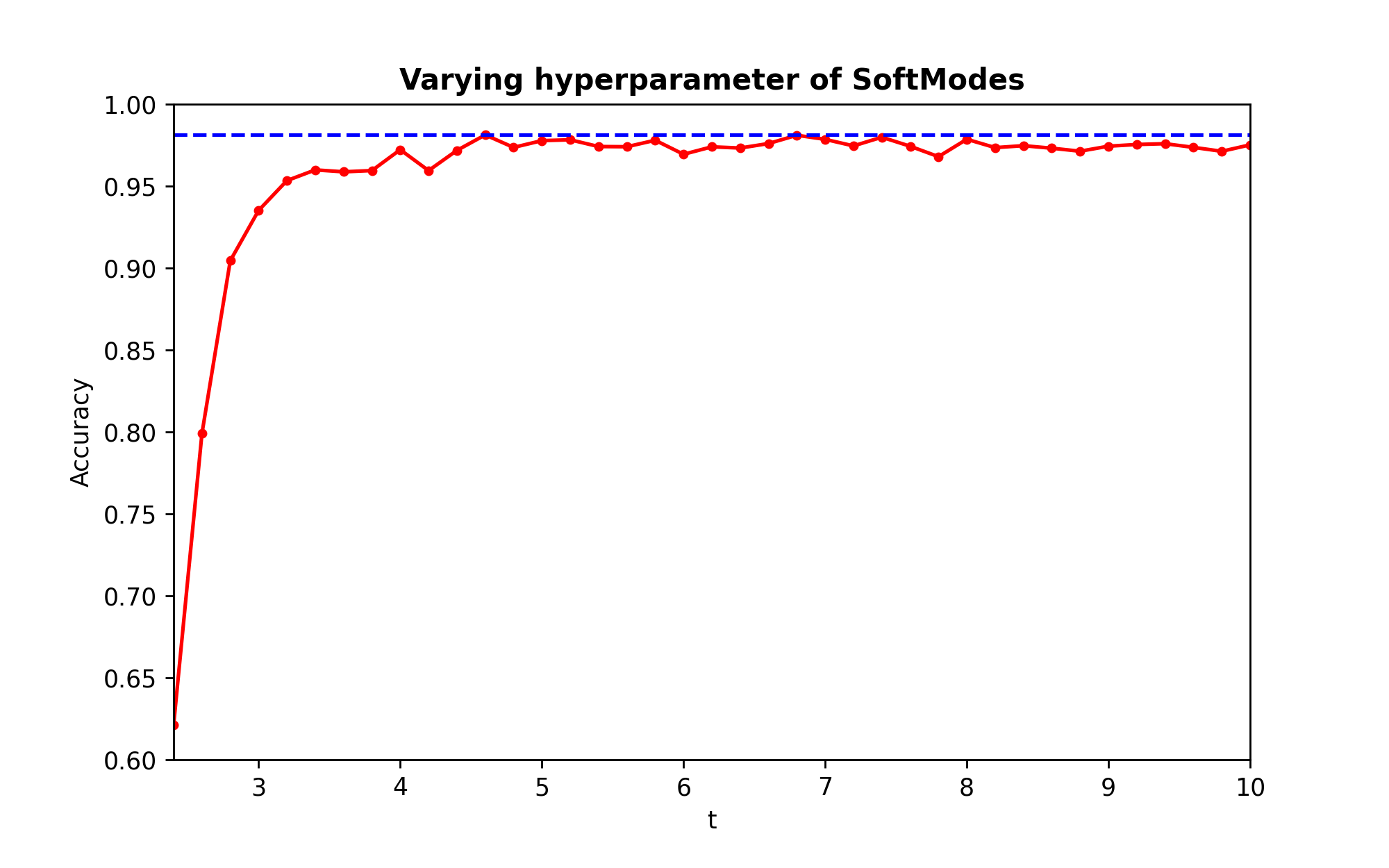
While -means converges slightly faster to its local minima than SoftModes in Figure 6a, the latter continues to make slow but steady progress. Also it is worth noting that rate of convergence of -modes is less than SoftModes. Finally, we remark that the hyperparameter is not very sensitive after a particular threshold is crossed (as seen in Figure 6b) and this is expected as the performance of SoftModes is lower bounded by the performance of -modes algorithm.
As a side note, we remark that SoftModes is sensitive to initialization and an initial seeding algorithm, like k-means++ seeding, does give observably better accuracy results than random seeding. Note that over the Hamming metric, the and sampling have identical distributions.
5 Conclusion
In this paper, we identified (theoretically and empirically) the poor performance of the -modes algorithm in the Boolean Block model. We remedied the situation by suggesting a soft rounding variant of -modes, namely, SoftModes. We remark that SoftModes, much like -means, and -modes can be parallelized to yield scalability. We leave it as an open question if one come up with a more sophisticated rounding family of functions for which one can theoretically prove constant factor approximation of the -modes objective. Another open question is to theoretically prove that SoftModes performs better than -means in the corrupted codewords model. Finally, it would be interesting to prove performance guarantees for SoftModeswhen , or remove the assumption on to be sufficiently small for the last conclusion in Theorem 3.1 to hold.
Acknowledgment
This work was supported by a grant from the Simons Foundation, Grant Number 825876, Awardee Thu D. Nguyen.
References
- [And14] Michael R Anderberg. Cluster analysis for applications: probability and mathematical statistics: a series of monographs and textbooks, volume 19. Academic press, 2014.
- [ATMS04] Periklis Andritsos, Panayiotis Tsaparas, Renée J. Miller, and Kenneth C. Sevcik. LIMBO: scalable clustering of categorical data. In Elisa Bertino, Stavros Christodoulakis, Dimitris Plexousakis, Vassilis Christophides, Manolis Koubarakis, Klemens Böhm, and Elena Ferrari, editors, Advances in Database Technology - EDBT 2004, 9th International Conference on Extending Database Technology, Heraklion, Crete, Greece, March 14-18, 2004, Proceedings, volume 2992 of Lecture Notes in Computer Science, pages 123–146. Springer, 2004.
- [BCK08] Shyam Boriah, Varun Chandola, and Vipin Kumar. Similarity measures for categorical data: A comparative evaluation. In Proceedings of the 2008 SIAM international conference on data mining, pages 243–254. SIAM, 2008.
- [Ber06] P. Berkhin. A Survey of Clustering Data Mining Techniques, pages 25–71. Springer Berlin Heidelberg, Berlin, Heidelberg, 2006.
- [BLC02] Daniel Barbará, Yi Li, and Julia Couto. COOLCAT: an entropy-based algorithm for categorical clustering. In Proceedings of the 2002 ACM CIKM International Conference on Information and Knowledge Management, McLean, VA, USA, November 4-9, 2002, pages 582–589. ACM, 2002.
- [Boc89] H. H. Bock. Probabilistic aspects in cluster analysis. In Otto Optiz, editor, Conceptual and Numerical Analysis of Data, pages 12–44, Berlin, Heidelberg, 1989. Springer Berlin Heidelberg.
- [CKL22] Vincent Cohen-Addad, Karthik C. S., and Euiwoong Lee. Johnson coverage hypothesis: Inapproximability of k-means and k-median in -metrics. In Joseph (Seffi) Naor and Niv Buchbinder, editors, Proceedings of the 2022 ACM-SIAM Symposium on Discrete Algorithms, SODA 2022, Virtual Conference / Alexandria, VA, USA, January 9 - 12, 2022, pages 1493–1530. SIAM, 2022.
- [CLLZ13] Fuyuan Cao, Jiye Liang, Deyu Li, and Xingwang Zhao. A weighting k-modes algorithm for subspace clustering of categorical data. Neurocomputing, 108:23–30, 2013.
- [CWJ07] Zhihua Cai, Dianhong Wang, and Liangxiao Jiang. K-distributions: A new algorithm for clustering categorical data. In De-Shuang Huang, Laurent Heutte, and Marco Loog, editors, Advanced Intelligent Computing Theories and Applications. With Aspects of Artificial Intelligence, Third International Conference on Intelligent Computing, ICIC 2007, Qingdao, China, August 21-24, 2007, Proceedings, volume 4682 of Lecture Notes in Computer Science, pages 436–443. Springer, 2007.
- [DG17] Dheeru Dua and Casey Graff. UCI machine learning repository, 2017.
- [GG91] Allen Gersho and Robert M. Gray. Vector quantization and signal compression, volume 159 of The Kluwer international series in engineering and computer science. Kluwer, 1991.
- [GGR99] Venkatesh Ganti, Johannes Gehrke, and Raghu Ramakrishnan. CACTUS - clustering categorical data using summaries. In Usama M. Fayyad, Surajit Chaudhuri, and David Madigan, editors, Proceedings of the Fifth ACM SIGKDD International Conference on Knowledge Discovery and Data Mining, San Diego, CA, USA, August 15-18, 1999, pages 73–83. ACM, 1999.
- [Git22] GitHub. http://github.com/sharath-cgm/SoftModes, 2022. [Online; accessed 18-October-2022].
- [Goo66] David W Goodall. A new similarity index based on probability. Biometrics, pages 882–907, 1966.
- [GRS99] Sudipto Guha, Rajeev Rastogi, and Kyuseok Shim. ROCK: A robust clustering algorithm for categorical attributes. In Masaru Kitsuregawa, Michael P. Papazoglou, and Calton Pu, editors, Proceedings of the 15th International Conference on Data Engineering, Sydney, Australia, March 23-26, 1999, pages 512–521. IEEE Computer Society, 1999.
- [HLL83] Paul W. Holland, Kathryn Blackmond Laskey, and Samuel Leinhardt. Stochastic blockmodels: First steps. Social Networks, 5(2):109–137, 1983.
- [HN99] Zhexue Huang and Michael K Ng. A fuzzy k-modes algorithm for clustering categorical data. IEEE transactions on Fuzzy Systems, 7(4):446–452, 1999.
- [HPHC21] Sibylle Hess, Gianvito Pio, Michiel E. Hochstenbach, and Michelangelo Ceci. BROCCOLI: overlapping and outlier-robust biclustering through proximal stochastic gradient descent. Data Min. Knowl. Discov., 35(6):2542–2576, 2021.
- [HPK+14] Ville Hautamäki, Antti Pöllänen, Tomi Kinnunen, Kong-Aik Lee, Haizhou Li, and Pasi Fränti. A comparison of categorical attribute data clustering methods. In Pasi Fränti, Gavin Brown, Marco Loog, Francisco Escolano, and Marcello Pelillo, editors, Structural, Syntactic, and Statistical Pattern Recognition - Joint IAPR International Workshop, S+SSPR 2014, Joensuu, Finland, August 20-22, 2014. Proceedings, volume 8621 of Lecture Notes in Computer Science, pages 53–62. Springer, 2014.
- [Hua97] Joshua Zhexue Huang. A fast clustering algorithm to cluster very large categorical data sets in data mining. In DMKD, 1997.
- [HW79] JA Hartigan and MA Wong. Algorithm AS 136: A K-means clustering algorithm. Applied Statistics, pages 100–108, 1979.
- [HXDD05] Zengyou He, Xiaofei Xu, Shengchun Deng, and Bin Dong. K-histograms: An efficient clustering algorithm for categorical dataset. CoRR, abs/cs/0509033, 2005.
- [Llo82] Stuart P. Lloyd. Least squares quantization in PCM. IEEE Trans. Inf. Theory, 28(2):129–136, 1982.
- [Mac67] J. Macqueen. Some methods for classification and analysis of multivariate observations. In In 5-th Berkeley Symposium on Mathematical Statistics and Probability, pages 281–297, 1967.
- [MMB09] Anirban Mukhopadhyay, Ujjwal Maulik, and Sanghamitra Bandyopadhyay. Multiobjective genetic algorithm-based fuzzy clustering of categorical attributes. IEEE Trans. Evol. Comput., 13(5):991–1005, 2009.
- [MN20] Pauli Miettinen and Stefan Neumann. Recent developments in boolean matrix factorization. In Christian Bessiere, editor, Proceedings of the Twenty-Ninth International Joint Conference on Artificial Intelligence, IJCAI 2020, pages 4922–4928. ijcai.org, 2020.
- [Nov19] Andrei Novikov. PyClustering: Data mining library. Journal of Open Source Software, 4(36):1230, apr 2019.
- [PVG+11] F. Pedregosa, G. Varoquaux, A. Gramfort, V. Michel, B. Thirion, O. Grisel, M. Blondel, P. Prettenhofer, R. Weiss, V. Dubourg, J. Vanderplas, A. Passos, D. Cournapeau, M. Brucher, M. Perrot, and E. Duchesnay. Scikit-learn: Machine learning in Python. Journal of Machine Learning Research, 12:2825–2830, 2011.
- [QLL+16] Yuhua Qian, Feijiang Li, Jiye Liang, Bing Liu, and Chuangyin Dang. Space structure and clustering of categorical data. IEEE Trans. Neural Networks Learn. Syst., 27(10):2047–2059, 2016.
- [Ros97] Sheldon M. Ross. Introduction to Probability Models. Academic Press, San Diego, CA, USA, sixth edition, 1997.
- [Smi68] E. S. Smirnov. On Exact Methods in Systematics. Systematic Biology, 17(1):1–13, 03 1968.
- [WKQ+08] Xindong Wu, Vipin Kumar, J. Ross Quinlan, Joydeep Ghosh, Qiang Yang, Hiroshi Motoda, Geoffrey J. McLachlan, Angus F. M. Ng, Bing Liu, Philip S. Yu, Zhi-Hua Zhou, Michael S. Steinbach, David J. Hand, and Dan Steinberg. Top 10 algorithms in data mining. Knowl. Inf. Syst., 14(1):1–37, 2008.
- [YKCQ15] Chao-Lung Yang, Ren-Jieh Kuo, Chia-Hsuan Chien, and Nguyen Thi Phuong Quyen. Non-dominated sorting genetic algorithm using fuzzy membership chromosome for categorical data clustering. Appl. Soft Comput., 30:113–122, 2015.
- [ZX18] Shuwei Zhu and Lihong Xu. Many-objective fuzzy centroids clustering algorithm for categorical data. Expert Syst. Appl., 96:230–248, 2018.