Contact-Implicit Planning and Control for Non-Prehensile Manipulation Using State-Triggered Constraints

The main contributions of our work are:

• •

  An automatic contact constraint activation (CA) method that triggers only the contact constraints useful for given task, thus reducing the problem’s sensitivity to the number of contact pairs and enabling automatic contact candidate assignment, i.e., all perceived surfaces can be assigned as contact candidates as they are handled efficiently in the optimization. Extensive simulations show that the proposed CA method improves the computational efficiency and the success rate.

• •

  We reformulate the Coulomb friction model using STCs and compare it to a baseline based on CCs for discovering tangential forces to rotate a box to random goal orientations. The proposed model is significantly faster and more robust than the baseline.

• •

  The STC-based friction model is used to model the contact modes of planar quasi-static pushing and compared to a MIP-based controller. Our method outperforms the baseline both in speed and accuracy. Moreover, the method can plan contact-interaction trajectories given only a desired state trajectory without any heuristics. Although our method may run slower than the learning-based variant hogan2020reactive, we demonstrate experimentally that our STC-based control can plan and track complex trajectories at a frequency high enough for real-time applications.

To the best of our knowledge, this is the first usage of STCs in contact modeling. We show that STCs hold immense promise for modeling discrete elements in this domain and can mitigate the need for explicit combinatorics and heuristics. Our proposed CA and friction methods serve as example applications for STCs. The extensive simulation and hardware experiments prove the efficacy of the proposed methodology.

Following stewart1996implicit, a contact impulse due to a frictionless inelastic collision between two rigid bodies can be modeled by $0\leq\phi(\mathbf{q})\perp\lambda_{n}\geq 0$; where the non-negativity condition for the signed distance $\phi(\mathbf{q})$ prevents interpenetration between bodies, and the non-negativity condition for the normal contact force $\lambda_{n}$ ensures that the contact bodies can only push each other. The frictional forces $\boldsymbol{\lambda}_{t}\in\mathbb{R}^{2}$ can be modeled using the relative tangential (slip) velocity in the contact frame $\psi(\mathbf{q},\dot{\mathbf{q}})$, the friction coefficient $\mu$ and by splitting tangential force into directional components $\lambda_{t}^{+},\lambda_{t}^{-}\geq 0$:

where $\gamma$ is an auxiliary variable corresponding to the absolute value of the slip velocity. It is noteworthy that this formulation is based on the maximization of the dissipation of kinetic energy subject to pyramidical friction cone constraints, see manchester2020variational for a derivation. However, the stationarity condition is neglected, and this leads to not being able to counteract external forces to prevent slippage when the slip velocity is zero. Nevertheless, these constraints are sufficient to ensure that the tangential forces selected by the planner are bounded by the friction polyhedron when sticking and counteracting at the boundary when slipping.

The CIP problem can be transcribed into a nonlinear program (NLP) for $N$ time steps of size $h$ using a backwards Euler discretization of the underactuated dynamics for an $n_{v}\triangleq n_{a}+n_{u}$ degrees-of-freedom (DOF) system with $n_{a}$ actuated and $n_{u}$ unactuated DOF:

where $\mathbf{q}\in\mathbb{R}^{n_{q}}$ and $\dot{\mathbf{q}}\in\mathbb{R}^{n_{v}}$ are the generalized positions and velocities of the system; $\mathbf{M}(\mathbf{q})\in\mathbb{R}^{n_{v}\times n_{v}}$ and $\mathbf{c}(\mathbf{q},\dot{\mathbf{q}})\in\mathbb{R}^{n_{v}}$ denote the mass matrix and the Coriolis, centrifugal, and gravitational terms; $\boldsymbol{\tau}\in\mathbb{R}^{n_{a}}$ is the vector of generalized joint forces; $\mathbf{S}_{a}\in\mathbb{R}^{n_{v}\times n_{a}}$ is the selection matrix for the actuated DOF; and $\boldsymbol{\lambda}_{c}\in\mathbb{R}^{3n_{c}}$ is the vector of contact forces for $n_{c}$ contacts that are projected onto the joint space through the contact Jacobian $\mathbf{J}_{c}(\mathbf{q}):\mathbb{R}^{n_{q}}\mapsto\mathbb{R}^{3n_{c}\times n_{v}}$. Representing the state by $\mathbf{x}\triangleq[\mathbf{q}^{T}\ \mathbf{\dot{q}}^{T}]^{T}\in\mathbb{R}^{n}$, $\mathbf{X}\triangleq[\mathbf{x}_{1},...,\mathbf{x}_{N+1}]$, $\mathbf{U}\triangleq[\boldsymbol{\tau}_{1},...,\boldsymbol{\tau}_{N}]$, $\mathbf{F}\triangleq[\boldsymbol{\lambda}_{1},...,\boldsymbol{\lambda}_{N}]$, $\mathbf{S}\triangleq[\mathbf{s}_{1},...,\mathbf{s}_{N+1}]$ are the state, control, force, and slack trajectories; and $\boldsymbol{\tau}_{L}$, $\boldsymbol{\tau}_{U}$, $\mathbf{x}_{L}$, and $\mathbf{x}_{U}$ are the lower and upper control and state bounds. The slack variables $\mathbf{s}$ are introduced to relax the CCs (including those for frictional forces) and penalized in the cost by an exact penalty function, as described in manchester2020variational; anitescu2005using. The constraints are evaluated element-wise posa2014direct.

In this work, we consider a single point pusher-slider system under the assumptions of quasi-static motion, Coulomb friction, and uniform pressure distribution over the support plane by following the formulation in hogan2016feedback. We model the dynamics of planar pushing using an ellipsoidal approximation of the limit surface goyal1991planar. We consider three contact modes between the pusher and the slider: sticking, sliding left, and sliding right. Each mode imposes a different set of friction constraints on the system. The planning problem can then be formulated as an MIP by linearizing the dynamics given desired state and control trajectories and a contact mode schedule. This framework is used to control the system in a receding horizon fashion such that the deviations from the nominal trajectories are minimized. We refer the reader to hogan2020reactive; hogan2016feedback for details.

An STC consists of a strict inequality trigger condition $g(\mathbf{x},\mathbf{u})<0$ and an inequality constraint condition $c(\mathbf{x},\mathbf{u})\leq 0$ such that

That is, the constraint $c(\mathbf{x},\mathbf{u})\leq 0$ becomes active if the trigger condition $g(\mathbf{x},\mathbf{u})<0$ is met. To include this logical implication in a smooth optimization problem, it must be represented using continuous variables, by introducing an auxiliary variable $\sigma\in\mathbb{R}_{++}$ and the following constraints

Given $(\mathbf{x},\mathbf{u})$, (4a) defines a linear complementarity problem in $\sigma$ which has a unique solution that can be obtained analytically as $\sigma^{*}=-\text{min}(g(\mathbf{x},\mathbf{u}),0)$. Plugging $\sigma^{*}$ into (4), we can obtain an STC that is continuous in $(\mathbf{x},\mathbf{u})$ – i.e., a continuous STC (cSTC) – as $-\text{min}(g(\mathbf{x},\mathbf{u}),0)\cdot c(\mathbf{x},\mathbf{u})\leq 0.$, see szmuk2020successive for details.

In the CC-based CITO, the constraint space grows with the number of contact pairs. Yet, at any instance, only a fraction of contact pairs are useful. Thus, we propose an automatic CA mechanism based on STCs that eliminates unnecessary contact pairs. This concept, based on a simple heuristic for planar pushing, is intended to showcase the versatility of STCs in this domain.

Fig. 1 illustrates the CA mechanism for a planar pushing scenario where $\mathbf{d}$ is the vector from the box’s current location to the desired. In this case, contact candidates are typically defined by pairing each end effector with each surface of the manipuland. However, the contact pairs that cannot generate normal forces to aid task completion can be deactivated by bounding the corresponding normal forces to zero. This is achieved by replacing the CCs in (2e) by the following STCs

where $\mathbf{N}\triangleq[\mathbf{n}_{1},...,\mathbf{n}_{n_{c}}]\in\mathbb{R}^{3\times n_{c}}$ and $\mathbf{n}$ denotes the surface normal. Note that when the normal force is set to zero, the tangential forces are also suppressed.

In addition to selectively activating contact pairs for manipulation, this mechanism can be used to activate contact constraints efficiently in a cluttered environment. For example, the distance between the manipuland and the environment being less than a threshold, $d_{thresh}$, can be used as the trigger condition to activate important contact pairs on the fly, i.e.,

This is somewhat similar to the collision constraint relaxation used in schulman2014motion when the distance is above a safety margin. It should be noted that the activation of constraints based on task utility, i.e., the addition of (5) into (2), is performed only for the contact pairs between the robot and the manipuland. Whereas, the activation of contact pairs that have a distance less than the threshold, i.e., the addition of (6) into (2), is performed for all contact pairs. Thus, contact interactions are enabled between all contact pairs throughout the optimization but in a computationally-efficient way.^** * Experiments demonstrating the distance-triggered contact pairs can be found in the accompanying video.

The Coulomb friction model can be expressed in terms of if-then conditions as

Such logical implications can be conveniently expressed using the following STCs

In contrast to the CC-based formulation in (1), taking the absolute value of the slip velocity $\gamma$ is not required here, since non-negativity constraints do not need to be enforced when using STCs. Moreover, the Coulomb friction law described in (7) is expressed sufficiently using only uni-directional implications. In the remainder, (1) is used for the CC-based friction model, and (8) is used for the STC-based friction model. Note that we use these friction models to model the friction only in contacts between the robot and the manipuland and not for support contacts due to the lack of physical fidelity described in 2.1.

Both of the presented friction models can be employed to capture the switching nature of the quasi-static pushing without discrete modeling such that the MIP-based pushing controller hogan2016feedback can be re-formulated as a direct NLP given only a desired state trajectory $\mathbf{X}_{d}\triangleq\mathbf{X}+\bar{\mathbf{X}}$:

where $\mathbf{Q}_{N}$, $\mathbf{Q}$, and $\mathbf{R}$ are weight matrices that adjust the penalization of the state deviation and the control effort. Either friction model can be incorporated by replacing $g(\mathbf{u}_{i})\leq 0$ by the corresponding constraints, (1) or (8). To exploit the structure of the problem, we use a large-scale sparse solver that allows warm-starting, i.e., SNOPT snopt. At each time step during execution, the initial control input $\mathbf{u}_{0}$ is executed, and the shifted solution is used as the initial guess for re-planning in a receding-horizon fashion.

This formulation also differs from the MIP approach as the optimization variables are the absolute state and control values instead of their variations, as shown in Fig. 2. A significant advantage of this approach is that a predefined contact mode schedule and control trajectory are unnecessary meaning the NLP-based approach can be used to plan a contact-interaction trajectory given only a desired state trajectory and using a trivial initial guess where the robot and the object are static.

Two non-prehensile manipulation tasks are designed to evaluate the proposed methodology: a translation-only task for the CA method and a rotation-only task for the friction models. We use a standard 6-DOF robot arm, UR3e from Universal Robots, and a cube with a side length of $0.1$ m and a mass of $0.6$ kg. The friction coefficient is 0.6 for contact pairs between the box and robot and 0.2 between the box and ground. The weights in (2) are set as $w_{1}=1$ and $w_{2}=10^{4}$. The size and number of time steps are selected as $h=0.05$ s and $N=20$.

We compare the NLP- and MIP-based controllers through simulation experiments using the following parameters for both: $h=0.3$ s, $N=35$, $\mathbf{Q}=10\ diag(3,3,0.1,0)$, $\mathbf{Q}_{N}=2000\ diag(3,3,0.1,0)$, and $\mathbf{R}=0.5\ diag(1,1,0.01)$. For the MIP-based controller, aggregated contact mode sections are used to accelerate the problem solving, as in hogan2020reactive.^†† † The number of steps associated with each section is $\{1,5,5,5,5,5,5,4\}$ and the contact mode weight matrix is $\mathbf{W}=0.1\ diag(0,1,1,1,1,1,1,1)$.

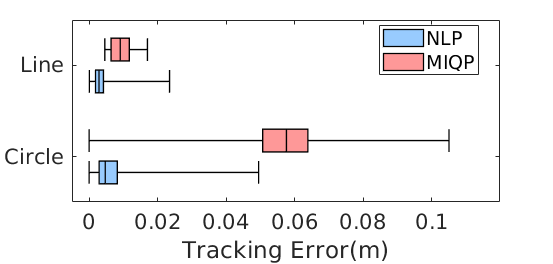
First, we consider a straight-line tracking scenario for a distance of $0.5$ m at a reference velocity of $0.05$ m/s. A feasible initial control trajectory is provided to both controllers. 100 simulations are performed with randomly-perturbed initial conditions that are drawn uniformly in the range $\pm[0.03,0.03,0.4,0.025]$. The computation time and tracking accuracy results are shown in Fig. 3. Overall, both controllers can handle the perturbations and accomplish the task. In this case, the NLP-based controller outperforms the MIP-based controller in all terms except for the maximum error bound. Second, an 8-shaped trajectory that consists of two circles of radius 0.15 m is tracked for 5 consecutive laps at a uniform desired angular velocity of 0.3 rad/s. However, in this case, a trivial infeasible control sequence is provided to the controller. The quantitative performances and the trajectories are shown in Figs. 3 and 4. The results show that the MIP-based controller cannot track the circular path accurately without a feasible nominal control sequence. This is likely caused by the linearized dynamics becoming ineffective for large deviations from the nominal trajectory. On the other hand, the NLP-based controller achieves precise tracking. Furthermore, the NLP can be solved within 0.02 s on average, which is promising for real-time applications.

References

- (1) Aceituno-Cabezas, B., Mastalli, C., Dai, H., Focchi, M., Radulescu, A., Caldwell, D.G., Cappelletto, J., Grieco, J.C., Fernández-López, G., Semini, C.: Simultaneous contact, gait, and motion planning for robust multilegged locomotion via mixed-integer convex optimization. IEEE Robotics and Automation Letters 3(3), 2531–2538 (2017)
- (2) Aceituno-Cabezas, B., Rodriguez, A.: A global quasi-dynamic model for contact-trajectory optimization. In: Robotics: Science and Systems (RSS) (2020)
- (3) Anitescu, M.: On using the elastic mode in nonlinear programming approaches to mathematical programs with complementarity constraints. SIAM Journal on Optimization 15(4), 1203–1236 (2005)
- (4) Carpentier, J., Mansard, N.: Analytical derivatives of rigid body dynamics algorithms. In: Robotics: Science and Systems (RSS) (2018)
- (5) Carpentier, J., Saurel, G., Buondonno, G., Mirabel, J., Lamiraux, F., Stasse, O., Mansard, N.: The Pinocchio C++ library – A fast and flexible implementation of rigid body dynamics algorithms and their analytical derivatives. In: IEEE International Symposium on System Integrations (SII) (2019)
- (6) Chatzinikolaidis, I., You, Y., Li, Z.: Contact-implicit trajectory optimization using an analytically solvable contact model for locomotion on variable ground. IEEE Robotics and Automation Letters 5(4), 6357–6364 (2020). DOI 10.1109/LRA.2020.3010754
- (7) Deits, R., Tedrake, R.: Footstep planning on uneven terrain with mixed-integer convex optimization. In: 2014 IEEE-RAS International Conference on Humanoid Robots, pp. 279–286. IEEE (2014)
- (8) Doshi, N., Hogan, F.R., Rodriguez, A.: Hybrid differential dynamic programming for planar manipulation primitives. In: 2020 IEEE International Conference on Robotics and Automation (ICRA), pp. 6759–6765. IEEE (2020)
- (9) Driess, D., Oguz, O., Ha, J.S., Toussaint, M.: Deep visual heuristics: Learning feasibility of mixed-integer programs for manipulation planning. In: 2020 IEEE International Conference on Robotics and Automation (ICRA) (2020)
- (10) Gabiccini, M., Artoni, A., Pannocchia, G., Gillis, J.: A computational framework for environment-aware robotic manipulation planning. In: Robotics Research, pp. 363–385. Springer (2018)
- (11) Gill, P.E., Murray, W., Saunders, M.A.: SNOPT: An SQP algorithm for large-scale constrained optimization. SIAM Rev. 47, 99–131 (2005)
- (12) Goyal, S., Ruina, A., Papadopoulos, J.: Planar sliding with dry friction part 1. limit surface and moment function. Wear 143(2), 307–330 (1991)
- (13) Gurobi Optimization, L.: Gurobi optimizer reference manual (2021). URL http://www.gurobi.com
- (14) Hogan, F.R., Rodriguez, A.: Feedback control of the pusher-slider system: A story of hybrid and underactuated contact dynamics. In: Proc. Workshop on the Algorithmic Foundations of Robotic (WAFR), pp. 800–815. Springer (2016)
- (15) Hogan, F.R., Rodriguez, A.: Reactive planar non-prehensile manipulation with hybrid model predictive control. The International Journal of Robotics Research 39(7), 755–773 (2020)
- (16) Kallwies, J., Forkel, B., Wuensche, H.J.: Determining and improving the localization accuracy of AprilTag detection. In: 2020 IEEE International Conference on Robotics and Automation (ICRA), pp. 8288–8294. IEEE (2020)
- (17) Li, W., Todorov, E.: Iterative linear quadratic regulator design for nonlinear biological movement systems. In: Proceedings of 1st International Conference on Informatics in Control, Automation, and Robotics (ICINCO), pp. 222–229 (2004)
- (18) Lynch, K.M., Mason, M.T.: Stable pushing: Mechanics, controllability, and planning. The Int. Journal of Robotics Research 15(6), 533–556 (1996)
- (19) Manchester, Z., Kuindersma, S.: Variational contact-implicit trajectory optimization. In: Robotics Research, pp. 985–1000. Springer (2020)
- (20) Mao, Y., Szmuk, M., Açıkmeşe, B.: Successive convexification of non-convex optimal control problems and its convergence properties. In: 2016 IEEE 55th Conference on Decision and Control (CDC), pp. 3636–3641. IEEE (2016)
- (21) Marcucci, T., Gabiccini, M., Artoni, A.: A two-stage trajectory optimization strategy for articulated bodies with unscheduled contact sequences. IEEE Robotics and Automation Letters 2(1), 104–111 (2017)
- (22) Marcucci, T., Tedrake, R.: Warm start of mixed-integer programs for model predictive control of hybrid systems. IEEE Transactions on Automatic Control (2020)
- (23) Mason, M.T.: Mechanics and planning of manipulator pushing operations. The International Journal of Robotics Research 5(3), 53–71 (1986)
- (24) Mastalli, C., Havoutis, I., Focchi, M., Caldwell, D.G., Semini, C.: Hierarchical planning of dynamic movements without scheduled contact sequences. In: 2016 IEEE International Conference on Robotics and Automation (ICRA), pp. 4636–4641. IEEE (2016)
- (25) Mordatch, I., Popović, Z., Todorov, E.: Contact-invariant optimization for hand manipulation. In: Proc. ACM SIGGRAPH/Eurographics Symposium on Computer Animation, pp. 137–144. Eurographics Association (2012)
- (26) Mordatch, I., Todorov, E., Popović, Z.: Discovery of complex behaviors through contact-invariant optimization. ACM Transactions on Graphics (TOG) 31(4), 43 (2012)
- (27) Neunert, M., Farshidian, F., Buchli, J.: Efficient whole-body trajectory optimization using contact constraint relaxation. In: 2016 IEEE-RAS 16th International Conference on Humanoid Robots (Humanoids), pp. 43–48. IEEE (2016)
- (28) Neunert, M., Stäuble, M., Giftthaler, M., Bellicoso, C.D., Carius, J., Gehring, C., Hutter, M., Buchli, J.: Whole-body nonlinear model predictive control through contacts for quadrupeds. IEEE Robotics and Automation Letters 3(3), 1458–1465 (2018)
- (29) Önol, A.Ö., Corcodel, R., Long, P., Padır, T.: Tuning-free contact-implicit trajectory optimization. In: 2020 IEEE International Conference on Robotics and Automation (ICRA), pp. 1183–1189. IEEE (2020)
- (30) Önol, A.Ö., Long, P., Padır, T.: A comparative analysis of contact models in trajectory optimization for manipulation. In: 2018 IEEE/RSJ International Conference on Intelligent Robots and Systems (IROS). IEEE (2018)
- (31) Önol, A.Ö., Long, P., Padır, T.: Contact-implicit trajectory optimization based on a variable smooth contact model and successive convexification. In: 2019 IEEE International Conference on Robotics and Automation (ICRA), pp. 2447–2453. IEEE (2019)
- (32) Patel, A., Shield, S.L., Kazi, S., Johnson, A.M., Biegler, L.T.: Contact-implicit trajectory optimization using orthogonal collocation. IEEE Robotics and Automation Letters 4(2), 2242–2249 (2019)
- (33) Posa, M., Cantu, C., Tedrake, R.: A direct method for trajectory optimization of rigid bodies through contact. The International Journal of Robotics Research 33(1), 69–81 (2014)
- (34) Reynolds, T., Szmuk, M., Malyuta, D., Mesbahi, M., Açıkmeşe, B., Carson, J.M.: A state-triggered line of sight constraint for 6-DOF powered descent guidance problems. In: AIAA Scitech 2019 Forum, p. 0924 (2019)
- (35) Reynolds, T.P., Szmuk, M., Malyuta, D., Mesbahi, M., Açıkmeşe, B., Carson III, J.M.: Dual Quaternion-Based Powered Descent Guidance with State-Triggered Constraints. Journal of Guidance, Control, and Dynamics 43(9), 1584–1599 (2020)
- (36) Schulman, J., Duan, Y., Ho, J., Lee, A., Awwal, I., Bradlow, H., Pan, J., Patil, S., Goldberg, K., Abbeel, P.: Motion planning with sequential convex optimization and convex collision checking. The International Journal of Robotics Research 33(9), 1251–1270 (2014)
- (37) Sleiman, J.P., Carius, J., Grandia, R., Wermelinger, M., Hutter, M.: Contact-Implicit Trajectory Optimization for Dynamic Object Manipulation. In: 2019 IEEE/RSJ International Conference on Intelligent Robots and Systems (IROS). IEEE (2019)
- (38) Stewart, D.E., Trinkle, J.C.: An implicit time-stepping scheme for rigid body dynamics with inelastic collisions and coulomb friction. International Journal for Numerical Methods in Engineering 39(15), 2673–2691 (1996)
- (39) Stouraitis, T., Yan, L., Moura, J., Gienger, M., Vijayakumar, S.: Multi-modal trajectory optimization for impact-aware manipulation. arXiv preprint arXiv:2006.13374 (2020)
- (40) Stüber, J., Zito, C., Stolkin, R.: Let’s push things forward: a survey on robot pushing. Frontiers in Robotics and AI 7, 8 (2020)
- (41) Szmuk, M., Malyuta, D., Reynolds, T.P., Mceowen, M.S., Açıkmeşe, B.: Real-Time Quad-Rotor Path Planning Using Convex Optimization and Compound State-Triggered Constraints. In: 2019 IEEE/RSJ International Conference on Intelligent Robots and Systems (IROS), pp. 7666–7673. IEEE (2019)
- (42) Szmuk, M., Reynolds, T., Açıkmeşe, B., Mesbahi, M., Carson, J.M.: Successive convexification for 6-DOF powered descent guidance with compound state-triggered constraints. In: AIAA Scitech 2019 Forum, p. 0926 (2019)
- (43) Szmuk, M., Reynolds, T.P., Açıkmeşe, B.: Successive Convexification for real-time six-degree-of-freedom powered descent guidance with state-triggered constraints. Journal of Guidance, Control, and Dynamics 43(8), 1399–1413 (2020)
- (44) Tassa, Y., Erez, T., Todorov, E.: Synthesis and stabilization of complex behaviors through online trajectory optimization. In: 2012 IEEE/RSJ International Conference on Intelligent Robots and Systems (IROS), pp. 4906–4913. IEEE (2012)
- (45) Wächter, A., Biegler, L.T.: On the implementation of an interior-point filter line-search algorithm for large-scale nonlinear programming. Mathematical programming 106(1), 25–57 (2006)
- (46) Wang, M., Luo, R., Önol, A.Ö., Padır, T.: Affordance-based mobile robot navigation among movable obstacles. In: 2020 IEEE/RSJ International Conference on Intelligent Robots and Systems (IROS). IEEE (2020)
- (47) Winkler, A.W.: IFOPT - Interface to nonlinear programming solvers IPOPT and SNOPT
- (48) Winkler, A.W., Bellicoso, C.D., Hutter, M., Buchli, J.: Gait and trajectory optimization for legged systems through phase-based end-effector parameterization. IEEE Robotics and Automation Letters 3(3), 1560–1567 (2018)
- (49) Yunt, K., Glocker, C.: Trajectory optimization of mechanical hybrid systems using SUMT. In: 9th IEEE International Workshop on Advanced Motion Control, pp. 665–671. IEEE (2005)
- (50) Zhou, J., Hou, Y., Mason, M.T.: Pushing revisited: Differential flatness, trajectory planning, and stabilization. The International Journal of Robotics Research 38(12-13), 1477–1489 (2019)