Photon Energy-Resolved Velocity Map Imaging from Spectral Domain Ghost Imaging
Abstract
We present an approach that combines photon spectrum correlation analysis with the reconstruction of three-dimensional momentum distribution from velocity map images in an efficient, single-step procedure. We demonstrate its efficacy with the results from the photoionization of the -shell of argon using the FLASH free-electron laser (FEL). Distinct spectral features due to the spin-orbit splitting of Ar are resolved, despite the large average bandwidth of the ionizing pulses from the FEL. This demonstrates a clear advantage over the conventional analysis method, and it will be broadly beneficial for velocity map imaging experiments with FEL sources. The retrieved linewidth of the binding energy spectrum approaches the resolution limitation prescribed by the spectrometers used to collect the data. Our approach presents a path to extend spectral-domain ghost imaging to the case where the photoproduct observable is high-dimensional.
I Introduction
Modern x-ray spectroscopy provides a sensitive probe of local electronic density in molecular systems with atomic-site specificity Siegbahn 1982; Picón et al. 2016; Erk et al. 2014. As a result, x-ray free-electron lasers (XFELs) with continuous wavelength tunability throughout the soft x-ray region, unparalleled peak brightness, and short temporal duration, have enabled significant advances in time-resolved measurements of molecular dynamics Wolf et al. 2017; Jay et al. 2022; Brauße et al. 2018; Allum et al. 2022. Oftentimes the intrinsic photon energy jitter of a self-amplified spontaneous emission (SASE) XFEL, along with the strongly fluctuating sub-structure, is thought to be the limiting factor for achievable energy resolution in time-resolved spectroscopy Brauße et al. 2018; Allum et al. 2022; Mayer et al. 2022. However, the spectral fluctuations inherent to SASE operation can, in fact, be exploited as a notable advantage by correlating x-ray observables with properties of the incident pulse on a shot-to-shot basis. This is a powerful approach to improving the resolution of experiments at XFEL facilities, beyond the bandwidth limit. In particular, the application of the spectral-domain ghost imaging (SDGI) technique has demonstrated sub-bandwidth resolution for spectroscopies employing XFELs Driver et al. 2020a; Li et al. 2021; Kayser et al. 2019; Klein et al. 2022.
Thanks to their high throughput, collection solid-angle, and ability to provide angle-resolved photoproduct yields, velocity map imaging (VMI) spectrometers Eppink and Parker 1997 have emerged as a popular instrument for time-resolved XFEL studies of dynamics in gas phase systems Erk et al. 2014; Squibb et al. 2018; Eppink and Parker 1997; Rouzée et al. 2011; Fushitani et al. 2021; Prince et al. 2016; Brauße et al. 2018; Allum et al. 2022. A VMI spectrometer typically measures the two-dimensional (2D) projection of the three-dimensional (3D) momentum distribution of charged particles. In most cases, however, the quantity of interest is the underlying 3D distribution or another related quantity such as the kinetic energy (KE) spectrum, access to which requires post-processing of the 2D projection that inverts the Abel transform Garcia et al. 2004; Roberts et al. 2009; Dick 2014; Montgomery Smith et al. 1988; Vrakking 2001. In trying to apply SDGI to retrieve the photon energy-resolved KE spectrum of charged particles from a VMI data set, the momentum projection, inherent to the VMI operation principal, could complicate the procedure. A feature with a specific KE is mapped to a broad range of pixels on the VMI detector, and thus features with distinct KEs will produce heavily overlapping features in the projected distribution This is in contrast with previous applications of SDGI, where KE is more directly related to the experimental measurement Li et al. 2021. In this work, we present a single-step regression approach which can simultaneously reconstruct the spectral response and the 3D momentum distribution by exploiting correlation between the single-shot VMI image and the corresponding photon spectrum demonstrating that the projection inherent in the VMI concept is not detrimental to the SDGI procedure.

The primary components of a typical experiment where correlation analysis can be applied is illustrated in Fig. 1. Briefly, a stochastic light source (here the SASE XFEL Feldhaus 2010) produces pulses that intercept a grating. The reflected beam (zeroth order) is directed toward the interaction point of a VMI spectrometer, which records the single-shot photoelectron momentum distribution. The incident spectrum is measured from the first order diffraction of the grating Brenner et al. 2011.
In Sec. II, we describe our single-step regression approach. In Sec. III, we demonstrate it with an experiment at the Free-electron LASer in Hamburg (FLASH), where spectral resolution below the average bandwidth of the incident x-ray pulses has been achieved. We point out that sub-bandwidth resolution is a common advantage of photon spectrum correlation analysis approaches. In Sec. IV, we describe the advantage we observe in regularizing with a single-step reconstruction compared to other possible implementations. Our approach promises to enhance the energy resolution of XFEL experiments using VMI, opening up opportunities to study time-dependent phenomena through the variation in finely resolved energy structures Inhester et al. 2019; Allum et al. 2022.
II Method
II.1 Model
The primary quantity of interest in VMI measurements is the 3D momentum distribution of charged particles, , which depends on the spectral profile of the incoming pulse, according to
| (1) |
where is the frequency spectrum of an incident pulse, and is the (linear) response to the spectral intensity at frequency . This model applies to light-matter interactions in the linear regime, such as single-photon ionization. The image obtained in a VMI spectrometer is given by the Abel transform of with a mapping from momentum to position ,
| (2) |
where is the direction of projection, is the magnification factor depending on the time-of-flight and particle mass , and is the -dependent momentum distribution.
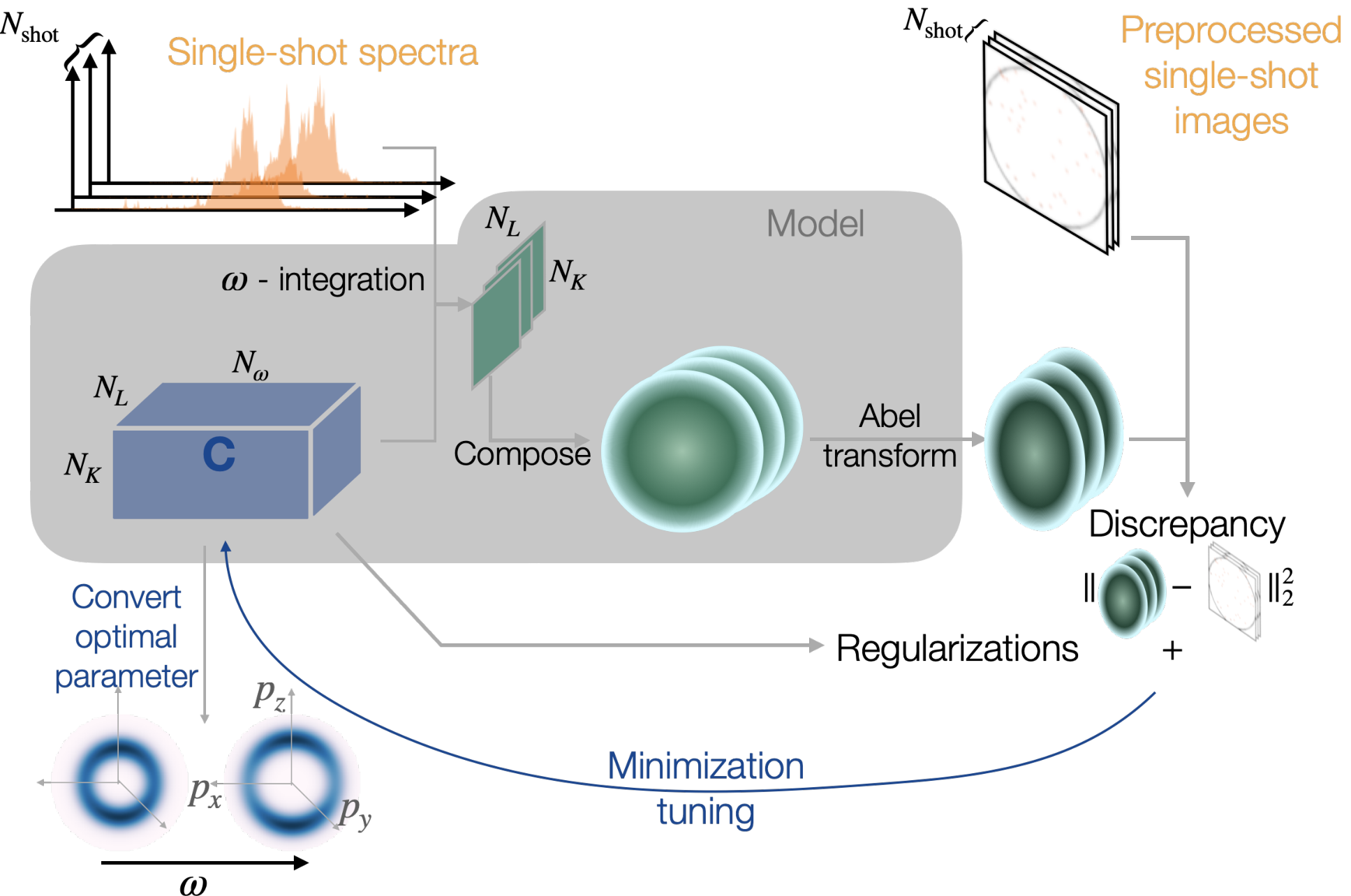
Our analysis approach is summarized graphically in Fig. 2. The spectral response of the sample, , is extracted by fitting a model to a combination of single-shot VMI images and photon spectra. The most likely is the function that minimizes the difference between the measured and predicted electron momentum distributions, subject to regularization terms that favor sparsity and smoothness in the -dependent distribution . We restrict our considerations to cases with cylindrical symmetry, where the axis of symmetry (), is oriented perpendicular to the direction of projection (), such as the case shown in Fig. 1. Other configurations satisfying the same symmetry requirements are discussed in Sec. IV.4 . Such a model is sufficient to describe experiments using either linearly- or circularly-polarized laser pulses acting on isotropic samples. The Abel transform is uniquely invertible under this symmetry condition, and the quality of the reconstruction will depend on the number of FEL shots used.
II.2 Implementation
In general, the inverse Abel transform is ill-conditioned, being susceptible to experimental noise Pretzier et al. 1992. Several inversion algorithms Garcia et al. 2004; Roberts et al. 2009; Dick 2014; Montgomery Smith et al. 1988; Vrakking 2001 have been developed to mitigate this issue and to robustly reconstruct the underlying 3D momentum distribution. In our method we adopt the basis functions employed in the well-known pBasex Garcia et al. 2004 algorithm to represent and combine the inversion procedure with spectral domain ghost imaging Driver et al. 2020a; Li et al. 2021. pBasex expands the three-dimensional momentum distribution with a basis set that is the product of radial basis functions and Legendre polynomials:
| (3) |
where is the -th order Legendre polynomial, and the sum over can be truncated at twice the highest order of light-matter interaction (i.e. twice the number of photons involved in the ionization process). is a set of radial basis functions, and are their -dependent coefficients.
Combining Eqn. (3) with Eqn. (2), the projected 2D distribution can be written as:
| (4) |
where , is the projection of each basis function perpendicular to the axis of cylindrical symmetry. It is worth noting, that after discretization on a Cartesian grid , the projections are the same integrals encountered in the standard pBasex inversion method (Eqn. 4 of Ref. Garcia et al. 2004). Being further uniformly discretized in photon energy , Eqn. (4) is
| (5) |
where for each single-shot, , is the expected intensity at pixel given the spectral profile and the spectral response of the sample encoded in the coefficients . Solving for the coefficients from the expected image is straightforward, as the tensor can be reshaped into a matrix , whose pseudo-inverse maps to . However, solving from the measured images by application of the pseudo-inverse, is highly sensitive to experimental noise in both and photon spectra . A more robust approach is to minimize an objective function, consisting of , which quantifies the model-measurement discrepancy, and regularization terms favoring expected qualities of , such as sparsity and smoothness Li et al. 2021, which is similar to the procedure discussed in Ref. Dick 2013. In our case, is
| (6) |
where
| (7) |
is the Gaussian log-likelihood up to a global factor, with weights over each pixel in the VMI image. Weights can be chosen to enhance the sensitivity of the reconstruction to certain regions of the VMI image, and henceforth we denote to be the diagonal matrix constructed by them. and are the sparsity and smoothness regularization terms, respectively.
We separate smoothness into two terms and , to differentiate the smoothness along the frequency (), and radial () directions. The corresponding hyperparameters, control the degree to which sparsity and smoothness are enforced in the retrieved . For each direction in , the smoothness term quantifies the roughness with the second order difference, i.e. , with representing the finite-difference Laplacian operator along direction . Common choices for the form of include the -norm Tibshirani 1996 and -norm squared Tikhonov et al. 1995. We choose the latter for the demonstration in Sec. III. We discuss strategies for choosing the proper values for the hyperparameters in the supplementary material.
From the point of view of implementation, the discrepancy term, , is quadratic in the coefficients, conducting the summation over shot to formulate into a quadratic form prior to the optimization significantly improves the efficiency, although at the cost of caching a large matrix in memory.
III Results

We demonstrate this reconstruction method for a dataset collected from soft x-ray ionization of argon above the ionization threshold Heimann et al. 1987; Avaldi et al. 1994a; Jurvansuu et al. 2001. The experiment is conducted using the CAMP instrument Erk et al. 2018 at beamline BL1 of the FLASH Feldhaus 2010. Argon gas is introduced via supersonic expansion to produce a continuous molecular beam. Following collimation through two skimmers and an aperture, the beam is intercepted by focused x-ray pulses produced by the FEL in the interaction region of the spectrometer. The velocities of the photoelectrons are mapped to a position-sensitive microchannel plate/phosphor screen detector and recorded with a CMOS camera at Hz.
The pulses have an average bandwidth of eV full-width at half maximum (FHWM) at eV central photon energy. The estimated pulse duration is fs (FWHM) with a mean pulse energy of J/pulse at the sample. The incident photon spectrum is recorded on a shot-to-shot basis using an upstream variable line spacing (VLS) spectrometer Brenner et al. 2011. The zeroth order beam from the grating is delivered to the interaction point, while the first order is collected by a detector to image the spectrum.

This measurement is performed with linearly polarized light from the FEL, which implies that the resulting electron momentum distribution has reflection symmetry about the plane. In this case, we can limit the sum in Eqn. (3) to only even-order Legendre polynomials Yang and Bersohn 1974. The dataset consists of FEL shots, and the representative single-shot raw VMI images and photon spectra are shown in Fig. 3, where the average VMI image and photon spectrum are also shown. The single-shot VMI images are quite sparse, containing 40 electrons in each image on average.
From the minimization of Eqn. (6), we obtain the most probable parameters given the dataset, which represents the fitted . Using Eqn. (5), the average image is reconstructed by averaging the expected intensity across all FEL shots. As shown in Fig. 3 (f), the reconstructed average image agrees well with the average of raw images except being less noisy. The reconstructed average image, nevertheless, is the projected momentum distribution of the mean photon spectrum and can hardly show the underlying fine structure. With the same set of most-probable parameters , a better way to reveal the fine structure is to reconstruct the KE spectrum for each -th Legendre polynomial component and each photon energy , which is discretized as
| (8) |
with denotes the KE at radial grid point . The ionization from argon -shell is a single-photon process, so we visualize and , in Fig. 4 (b)(c) respectively.
We observe two dispersive features that correspond to the spin-orbit split cationic states of argon, and Jurvansuu et al. 2001. For each photon energy in Fig. 4 (b), we shift the reconstructed KE spectrum to binding energy (BE) according to , which is shown in Fig. 4 (e). The spin-orbit splitting is well resolved with our approach. We use a previously reported measurement Jurvansuu et al. 2001 of this splitting, eV, to calibrate the VMI and VLS energy axes. With this calibration, we extract a line-width of eV FWHM from Fig. 4 (e), which is resolved beyond the width of the averaged FEL pulse spectrum, eV FWHM. Furthermore, the extracted line-width is below the average bandwidth of a single pulse eV FWHM. Thus, with the application of spectral domain ghost imaging in this XFEL experiment, we are able to achieve sub-bandwidth resolution.
In Fig. 4 (c) and (f) we plot the projection of the 3D momentum distribution onto the second-order Legendre polynomial , which is related to the photoemission anisotropy parameter, Cooper and Zare 1968. We extract a value of and for the anisotropy parameter for the and ionic states, respectively. These values are averaged over a range of photon energies from to eV, which is in good agreement with previous measurements in Ref. Avaldi et al. 1994b and calculations in Ref. Lindle et al. 1988. The results in Fig. 4 (b)(c)(e)(f) are obtained with a set of radial basis functions and uniform pixel weight .
In contrast, directly applying pBasex on the cumulative image results in a single spectral feature with a width of eV FWHM. Moreover, grouping the FEL shots by the centre-of-mass of photon spectrum does not resolve the two spin-orbit features, and the corresponding average binding energy spectrum has a width of eV (FWHM), as shown in Fig. 4 (a) and (d). In order to obtain the resolution observed in Fig. 4 (b) and (c), we need to explicitly consider the correlations between the single-shot spectra and the VMI images.
IV Discussion
IV.1 Resolution achieved in our demonstration experiment
To characterize the resolution of this technique, it is useful to define the correlation length of the spectral measurement. The correlation length is a measure of how strongly coupled the intensity fluctuations are between neighboring pixels in the photon spectrum. Here, we define this metric to be the average distance between two frequencies where the Pearson’s correlation coefficient drops to Driver et al. 2020b. The correlation between spectrometer pixels arises from two sources: the resolution of the photon spectrometer, and the intrinsic variation due to spectral fluctuations of the source. In our experiment, the correlation length is measured to be VLS pixels, corresponding to eV, as shown in Fig. S1(a) of the supplementary material. This is much larger than the instrumental resolution of the photon spectrometer Brenner et al. 2011, and thus, we conclude that the dominant contribution to the correlation length is the intrinsic correlation of the FEL source.
The average width of the photoemission features in the BE spectrum in Fig. 4 (e) is determined to be in standard deviation. This width is the result of the finite VMI energy resolution and the correlation in the spectral measurement, which approximately sum in quadrature . The contribution from spectral correlation, , is not necessarily the correlation length , but the two quantities are related by a constant of proportionality. As described in the supplemental material, and shown in Fig. S1(b), is estimated to be based on the measured px. Having accounted for , we find the remaining contribution to to be . This corresponds to a VMI energy resolution of 2.3% at , which is consistent with the reported value of 2% for this instrument Erk et al. 2018. We note that the average bandwidth of incident x-ray pulses is not a limiting factor for the resolution of our technique. Instead, it is determined by the kinetic energy resolution of the VMI spectrometer and the correlation length of the photon spectrum measurement.
IV.2 Extension of SDGI
Spectral domain ghost imaging, in general, exploits spectral fluctuations of the incident source to capture the sample response. The key development in the present work is incorporating the native projection of VMI into the ghost imaging model. This method unravels the projection of different Newton spheres, while simultaneously correlating these unravelled shells with the incident photon spectra. More specifically, our approach models the photoproduct momentum space with a reduced dimensional representation (similar to the pBasex approach) and inverts the tensor product of spectral integration and Abel transform in a single step. Such an approach is a unique way to extend the scope of SDGI. Although under ideal circumstances it is equivalent to conducting the two regression steps sequentially, the single-step approach has several advantages over either sequential approach.
In comparison to the sequential application of SDGI followed by Abel inversion, the single-step approach represents the momentum distribution with a polar basis set, reducing the dimensionality of the problem and coordinating the comprehensive behavior of the momentum distribution over multiple pixels. When applying SDGI directly to the 2D VMI data, incorporating the smoothness term that penalizes high spatial frequencies in momentum space is inefficient and in most cases intractable. This is because the dimension of the image space is too large. Conceding this smoothness over momentum space, we can implement a sequential approach by applying SDGI to each VMI pixel independently and subsequently applying pBasex to the result. This approach remains efficient, but it is plagued by compromised performance in noise handling, as shown in the supplementary material Fig. S2. The key difference between this sequential approach and the single-step is that the regression is performed independently for each pixel in the first of the two sequential steps.
Another feasible sequential approach is to apply single-shot Abel inversion followed by SDGI. Although the regularization terms can remain in the same form as in the single-step approach, in this approach the Gaussian log-likelihood in the objective function (Eqn. 6) is replaced by,
| (9) |
where is the pseudo-inverse of the Abel transform, which is conducted separately for each photon energy bin.
In our demonstration experiment, both sequential approaches show inferior performance compared to the single-step approach, which is illustrated in the comparison in the supplementary material. Under ideal circumstances, when regularization becomes unnecessary to suppress experimental noise, the optimal point of the original objective function in Eqn. (6) is
| (10a) | |||||
| (10b) | |||||
where , and in going from Eqn. (10a) to (10b) we have changed the order of operations between the pseudo-inverse and tensor-product of and . Equation (10a) describes the single-step approach and Eqn. (10b) denotes both the sequential approaches described above. Thus it can be seen that in the absence of regularization, both sequential approaches are equivalent to the single-step method. The regularization in Eqn. (6) necessitates the computationally heavy step of inverting an -dimensional matrix, which is not true for the sequential approaches. However, as described above, the single-step outperforms the sequential approaches by virtue of being more robust to noise. Similar results between the single-step and sequential approaches may be achieved in other measurements, and the precise choice of method depends critically on the properties of the measurement; e.g. signal-to-noise ratio, size of the dataset, and number of parameters to fit.
IV.3 Connection to Covariance Approach
We note that there are a number of mathematical techniques to extract correlations in large datasets. While the method presented in this work relies on linear regression, covariance analysis is another common method for extracting correlations Frasinski et al. 1989; Frasinski et al. 2013; Frasinski 2016; Allum et al. 2022; Amiot et al. 2018. The photoproduct yield can be correlated with other intrinsic or extrinsic measurements, to extract signal from noisy data. Both regression and covariance have been employed in ghost imaging experiments in the spectral domain, and these two techniques are closely related.
The connection is shown by regressing the mean-subtracted VMI images on the mean-subtracted spectra , with denoting the average across all shots. Given the standard definition of sample covariance , the unregularized spectral regression of on gives
| (11) |
where the right hand equality demonstrates this is identical to applying the inverse of the photon autocovariance matrix to the photon-electron covariance matrix.
The transform from the projected momentum distribution to the coefficients is a linear operation in the electron momentum space, which is in tensor product with the operations in the photon energy space. Therefore the aforementioned single-step and sequential regression approaches are all applicable to the mean-subtracted data. Comparing to the original approach elaborated in Sec. II, regressing the mean-subtracted data is more robust to static background in both the VMI images and photon spectra, but it may suffer from the loss of information due to subtraction of the mean, especially when the spectral fluctuation is limited. Regardless whether the mean is subtracted or not, one can further constrain the parameters with additional prior knowledge about the sample, to solve the most probable parameters in a space with dimension lower than . Although related, these further restricted approaches require more assumptions and are less generalisable than the main approach we present in this work. We provide an example in the supplementary material.
IV.4 Applicable Apparatus Configurations
As for standard inverse Abel transform procedures, a prerequisite of our method is the cylindrical symmetry about any axis that is perpendicular to the projection axis of the VMI , for which the coordinate system shown in Fig. 1 is not the only configuration. Here we describe two other configurations without exhausting all possible cases. For circularly polarized x-rays, such as in Ilchen et al. 2021, the layout in Fig. 1 is still applicable except that the symmetry axis is along the axis of beam propagation. For a co-axial VMI Li et al. 2018 with linearly polarized x-rays propagating along the VMI axis , falls along the x-ray polarization axis.
V Conclusion and Outlook
We present a regression approach which can achieve VMI measurements at resolution better than the inherent bandwidth of a noisy photon source, by simultaneously reconstructing the spectral response and performing the inverse Abel transform. Our approach demonstrates a clear advantage over the conventional binning-and-averaging method. In our experimental demonstration on the photoionization of argon, the retrieved linewidth is dominated by the resolution limit prescribed by the VMI resolution and the measured spectral correlation. We anticipate that the outlined approach will be of great use in the emerging field of time-resolved inner-shell photoelectron spectroscopy at FELs, which promises to interrogate photoinduced nuclear and electronic dynamics in a site-selective manner.
We demonstrate the connection between covariance and regression analysis and we relate and compare our single-step approach to other sequential approaches. Our method extends the scope of SDGI by adopting a reduced dimensional representation for the properties of the photoproducts, and it can be directly applied to any measurement where VMI images are recorded in coincidence with the incident photon spectrum. This makes the technique broadly applicable to many different light sources.
VI Data Availability
The data that support the findings of this study are available from the authors upon reasonable request. An implementation of the proposed approach can be found in our custom package developed for general SDGI Wang 2022.
VII Author Contributions
T.C.D., J.P.C and R.F. initiated the research. J.W., T.C.D. and J.P.C conceived the method, which is implemented by J.W. The experiment was carried out by C.C.P., C.P., G.B., S.D., A.T.N., S.K., and B.E. . All authors contributed to collection or analysis of the experimental data and writing of the manuscript.
VIII Acknowledgement
We acknowledge the Max Planck Society for funding the development and the initial operation of the CAMP end-station within the Max Planck Advanced Study Group at CFEL and for providing this equipment for CAMP@FLASH. The installation of CAMP@FLASH was partially funded by the BMBF grants 05K10KT2, 05K13KT2, 05K16KT3 and 05K10KTB from FSP-302. The analysis work was supported by the U.S. Department of Energy (DOE), Office of Science, Office of Basic Energy Sciences (BES), Chemical Sciences, Geosciences, and Biosciences Division (CSGB). We acknowledge DESY (Hamburg, Germany), a member of the Helmholtz Association HGF, for the provision of experimental facilities. Parts of this research were carried out at FLASH and the Maxwell computational resources operated at Deutsches Elektronen-Synchrotron DESY, Hamburg, Germany. We thank Jordan O’Neal and Alice E. Green for fruitful discussions.
References
- Siegbahn (1982) K. Siegbahn, Reviews of Modern Physics 54, 709 (1982).
- Picón et al. (2016) A. Picón, C. S. Lehmann, C. Bostedt, A. Rudenko, A. Marinelli, T. Osipov, D. Rolles, N. Berrah, C. Bomme, M. Bucher, G. Doumy, B. Erk, K. R. Ferguson, T. Gorkhover, P. J. Ho, E. P. Kanter, B. Krässig, J. Krzywinski, A. A. Lutman, A. M. March, D. Moonshiram, D. Ray, L. Young, S. T. Pratt, and S. H. Southworth, Nature Communications 7, 11652 (2016).
- Erk et al. (2014) B. Erk, R. Boll, S. Trippel, D. Anielski, L. Foucar, B. Rudek, S. W. Epp, R. Coffee, S. Carron, S. Schorb, K. R. Ferguson, M. Swiggers, J. D. Bozek, M. Simon, T. Marchenko, J. Küpper, I. Schlichting, J. Ullrich, C. Bostedt, D. Rolles, and A. Rudenko, Science 345, 288 (2014).
- Wolf et al. (2017) T. J. A. Wolf, R. H. Myhre, J. P. Cryan, S. Coriani, R. J. Squibb, A. Battistoni, N. Berrah, C. Bostedt, P. Bucksbaum, G. Coslovich, R. Feifel, K. J. Gaffney, J. Grilj, T. J. Martinez, S. Miyabe, S. P. Moeller, M. Mucke, A. Natan, R. Obaid, T. Osipov, O. Plekan, S. Wang, H. Koch, and M. Gühr, Nature Communications 8, 29 (2017).
- Jay et al. (2022) R. M. Jay, K. Kunnus, P. Wernet, and K. J. Gaffney, Annual Review of Physical Chemistry 73, annurev (2022).
- Brauße et al. (2018) F. Brauße, G. Goldsztejn, K. Amini, R. Boll, S. Bari, C. Bomme, M. Brouard, M. Burt, B. C. de Miranda, S. Düsterer, B. Erk, M. Géléoc, R. Geneaux, A. S. Gentleman, R. Guillemin, I. Ismail, P. Johnsson, L. Journel, T. Kierspel, H. Köckert, J. Küpper, P. Lablanquie, J. Lahl, J. W. L. Lee, S. R. Mackenzie, S. Maclot, B. Manschwetus, A. S. Mereshchenko, T. Mullins, P. K. Olshin, J. Palaudoux, S. Patchkovskii, F. Penent, M. N. Piancastelli, D. Rompotis, T. Ruchon, A. Rudenko, E. Savelyev, N. Schirmel, S. Techert, O. Travnikova, S. Trippel, J. G. Underwood, C. Vallance, J. Wiese, M. Simon, D. M. P. Holland, T. Marchenko, A. Rouzée, and D. Rolles, Physical Review A 97, 043429 (2018).
- Allum et al. (2022) F. Allum, V. Music, L. Inhester, R. Boll, B. Erk, P. Schmidt, T. M. Baumann, G. Brenner, M. Burt, P. V. Demekhin, S. Dörner, A. Ehresmann, A. Galler, P. Grychtol, D. Heathcote, D. Kargin, M. Larsson, J. W. L. Lee, Z. Li, B. Manschwetus, L. Marder, R. Mason, M. Meyer, H. Otto, C. Passow, R. Pietschnig, D. Ramm, K. Schubert, L. Schwob, R. D. Thomas, C. Vallance, I. Vidanovic, C. von Korff Schmising, R. Wagner, P. Walter, V. Zhaunerchyk, D. Rolles, S. Bari, M. Brouard, and M. Ilchen, Communications Chemistry 5, 42 (2022).
- Mayer et al. (2022) D. Mayer, F. Lever, D. Picconi, J. Metje, S. Alisauskas, F. Calegari, S. Düsterer, C. Ehlert, R. Feifel, M. Niebuhr, et al., Nature communications 13, 1 (2022).
- Driver et al. (2020a) T. Driver, S. Li, E. G. Champenois, J. Duris, D. Ratner, T. J. Lane, P. Rosenberger, A. Al-Haddad, V. Averbukh, T. Barnard, N. Berrah, C. Bostedt, P. H. Bucksbaum, R. Coffee, L. F. DiMauro, L. Fang, D. Garratt, A. Gatton, Z. Guo, G. Hartmann, D. Haxton, W. Helml, Z. Huang, A. LaForge, A. Kamalov, M. F. Kling, J. Knurr, M.-F. Lin, A. A. Lutman, J. P. MacArthur, J. P. Marangos, M. Nantel, A. Natan, R. Obaid, J. T. O’Neal, N. H. Shivaram, A. Schori, P. Walter, A. Li Wang, T. J. A. Wolf, A. Marinelli, and J. P. Cryan, Phys. Chem. Chem. Phys. 22, 2704 (2020a).
- Li et al. (2021) S. Li, T. Driver, A. A. Haddad, E. G. Champenois, M. Agåker, O. Alexander, T. Barillot, C. Bostedt, D. Garratt, L. Kjellsson, A. A. Lutman, J.-E. Rubensson, C. Sathe, A. Marinelli, J. P. Marangos, and J. P. Cryan, Journal of Physics B: Atomic, Molecular and Optical Physics 54, 144005 (2021).
- Kayser et al. (2019) Y. Kayser, C. Milne, P. Juranić, L. Sala, J. Czapla-Masztafiak, R. Follath, M. Kavčič, G. Knopp, J. Rehanek, W. Błachucki, et al., Nature communications 10, 1 (2019).
- Klein et al. (2022) Y. Klein, E. Strizhevsky, F. Capotondi, D. D. Angelis, L. Giannessi, M. Pancaldi, E. Pedersoli, G. Penco, K. C. Prince, O. Sefi, Y. Y. Kim, I. A. Vartanyants, and S. Shwartz, “High-resolution absorption measurements with free-electron lasers using ghost spectroscopy,” (2022), arXiv:2203.00688 .
- Eppink and Parker (1997) A. T. J. B. Eppink and D. H. Parker, Review of Scientific Instruments 68, 3477 (1997).
- Squibb et al. (2018) R. J. Squibb, M. Sapunar, A. Ponzi, R. Richter, A. Kivimäki, O. Plekan, P. Finetti, N. Sisourat, V. Zhaunerchyk, T. Marchenko, L. Journel, R. Guillemin, R. Cucini, M. Coreno, C. Grazioli, M. Di Fraia, C. Callegari, K. C. Prince, P. Decleva, M. Simon, J. H. D. Eland, N. Došlić, R. Feifel, and M. N. Piancastelli, Nature Communications 9, 63 (2018).
- Rouzée et al. (2011) A. Rouzée, P. Johnsson, E. V. Gryzlova, H. Fukuzawa, A. Yamada, W. Siu, Y. Huismans, E. Louis, F. Bijkerk, D. M. P. Holland, A. N. Grum-Grzhimailo, N. M. Kabachnik, M. J. J. Vrakking, and K. Ueda, Phys. Rev. A 83, 031401 (2011).
- Fushitani et al. (2021) M. Fushitani, S. T. Pratt, D. You, S. Saito, Y. Luo, K. Ueda, H. Fujise, A. Hishikawa, H. Ibrahim, F. Légaré, P. Johnsson, J. Peschel, E. R. Simpson, A. Olofsson, J. Mauritsson, P. A. Carpeggiani, P. K. Maroju, M. Moioli, D. Ertel, R. Shah, G. Sansone, T. Csizmadia, M. Dumergue, N. G. Harshitha, S. Kühn, C. Callegari, O. Plekan, M. Di Fraia, M. B. Danailov, A. Demidovich, L. Giannessi, L. Raimondi, M. Zangrando, G. De Ninno, P. R. Ribič, and K. C. Prince, The Journal of Chemical Physics 154, 144305 (2021), https://doi.org/10.1063/5.0046577 .
- Prince et al. (2016) K. C. Prince, E. Allaria, C. Callegari, R. Cucini, G. D. Ninno, S. D. Mitri, B. Diviacco, E. Ferrari, P. Finetti, D. Gauthier, L. Giannessi, N. Mahne, G. Penco, O. Plekan, L. Raimondi, P. Rebernik, E. Roussel, C. Svetina, M. Trovò, M. Zangrando, M. Negro, P. Carpeggiani, M. Reduzzi, G. Sansone, A. N. Grum-Grzhimailo, E. V. Gryzlova, S. I. Strakhova, K. Bartschat, N. Douguet, J. Venzke, D. Iablonskyi, Y. Kumagai, T. Takanashi, K. Ueda, A. Fischer, M. Coreno, F. Stienkemeier, Y. Ovcharenko, T. Mazza, and M. Meyer, Nature Photonics 10, 176 (2016).
- Garcia et al. (2004) G. A. Garcia, L. Nahon, and I. Powis, Review of Scientific Instruments 75, 4989 (2004).
- Roberts et al. (2009) G. M. Roberts, J. L. Nixon, J. Lecointre, E. Wrede, and J. R. R. Verlet, Review of Scientific Instruments 80, 053104 (2009).
- Dick (2014) B. Dick, Phys. Chem. Chem. Phys. 16, 570 (2014).
- Montgomery Smith et al. (1988) L. Montgomery Smith, D. R. Keefer, and S. Sudharsanan, Journal of Quantitative Spectroscopy and Radiative Transfer 39, 367 (1988).
- Vrakking (2001) M. J. J. Vrakking, Review of Scientific Instruments 72, 4084 (2001).
- Feldhaus (2010) J. Feldhaus, Journal of Physics B: Atomic, Molecular and Optical Physics 43, 194002 (2010).
- Brenner et al. (2011) G. Brenner, S. Kapitzki, M. Kuhlmann, E. Ploenjes, T. Noll, F. Siewert, R. Treusch, K. Tiedtke, R. Reininger, M. Roper, et al., Nuclear Instruments and Methods in Physics Research Section A: Accelerators, Spectrometers, Detectors and Associated Equipment 635, S99 (2011).
- Inhester et al. (2019) L. Inhester, Z. Li, X. Zhu, N. Medvedev, and T. J. A. Wolf, The Journal of Physical Chemistry Letters 10, 6536 (2019), publisher: American Chemical Society.
- Pretzier et al. (1992) G. Pretzier, H. Jäger, T. Neger, H. Philipp, and J. Woisetschläger, Zeitschrift für Naturforschung A 47, 955 (1992).
- Dick (2013) B. Dick, Physical Chemistry Chemical Physics 16, 570 (2013).
- Tibshirani (1996) R. Tibshirani, Journal of the Royal Statistical Society. Series B (Methodological) 58, 267 (1996).
- Tikhonov et al. (1995) A. N. Tikhonov, A. V. Goncharsky, V. V. Stepanov, and A. G. Yagola, “Regularization methods,” in Numerical Methods for the Solution of Ill-Posed Problems (Springer Netherlands, Dordrecht, 1995) pp. 7–63.
- Heimann et al. (1987) P. Heimann, D. Lindle, T. Ferrett, S. Liu, L. Medhurst, M. Piancastelli, D. Shirley, U. Becker, H. Kerkhoff, B. Langer, et al., Journal of Physics B: Atomic and Molecular Physics (1968-1987) 20, 5005 (1987).
- Avaldi et al. (1994a) L. Avaldi, G. Dawber, R. Camilloni, G. King, M. Roper, M. Siggel, G. Stefani, and M. Zitnik, Journal of Physics B: Atomic, Molecular and Optical Physics 27, 3953 (1994a).
- Jurvansuu et al. (2001) M. Jurvansuu, A. Kivimäki, and S. Aksela, Physical Review A 64, 012502 (2001).
- Erk et al. (2018) B. Erk, J. P. Müller, C. Bomme, R. Boll, G. Brenner, H. N. Chapman, J. Correa, S. Düsterer, S. Dziarzhytski, S. Eisebitt, et al., Journal of synchrotron radiation 25, 1529 (2018).
- Yang and Bersohn (1974) S.-c. Yang and R. Bersohn, The Journal of Chemical Physics 61, 4400 (1974).
- Cooper and Zare (1968) J. Cooper and R. N. Zare, The Journal of Chemical Physics 48, 942 (1968).
- Avaldi et al. (1994b) L. Avaldi, G. Dawber, R. Camilloni, G. C. King, M. Roper, M. R. F. Siggel, G. Stefani, and M. Zitnik, Journal of Physics B: Atomic, Molecular and Optical Physics 27, 3953 (1994b).
- Lindle et al. (1988) D. W. Lindle, L. J. Medhurst, T. A. Ferrett, P. A. Heimann, M. N. Piancastelli, S. H. Liu, D. A. Shirley, T. A. Carlson, P. C. Deshmukh, G. Nasreen, and S. T. Manson, Phys. Rev. A 38, 2371 (1988).
- Driver et al. (2020b) T. Driver, S. Li, E. G. Champenois, J. Duris, D. Ratner, T. J. Lane, P. Rosenberger, A. Al-Haddad, V. Averbukh, T. Barnard, N. Berrah, C. Bostedt, P. H. Bucksbaum, R. Coffee, L. F. DiMauro, L. Fang, D. Garratt, A. Gatton, Z. Guo, G. Hartmann, D. Haxton, W. Helml, Z. Huang, A. LaForge, A. Kamalov, M. F. Kling, J. Knurr, M.-F. Lin, A. A. Lutman, J. P. MacArthur, J. P. Marangos, M. Nantel, A. Natan, R. Obaid, J. T. O’Neal, N. H. Shivaram, A. Schori, P. Walter, A. L. Wang, T. J. A. Wolf, A. Marinelli, and J. P. Cryan, Physical Chemistry Chemical Physics 22, 2704 (2020b), publisher: The Royal Society of Chemistry.
- Frasinski et al. (1989) L. Frasinski, K. Codling, and P. Hatherly, Science 246, 1029 (1989).
- Frasinski et al. (2013) L. Frasinski, V. Zhaunerchyk, M. Mucke, R. J. Squibb, M. Siano, J. H. Eland, P. Linusson, P. Vd Meulen, P. Salén, R. Thomas, et al., Physical review letters 111, 073002 (2013).
- Frasinski (2016) L. J. Frasinski, Journal of Physics B: Atomic, Molecular and Optical Physics 49, 152004 (2016).
- Amiot et al. (2018) C. Amiot, P. Ryczkowski, A. T. Friberg, J. M. Dudley, and G. Genty, Optics Letters 43, 5025 (2018), publisher: Optica Publishing Group.
- Ilchen et al. (2021) M. Ilchen, P. Schmidt, N. M. Novikovskiy, G. Hartmann, P. Rupprecht, R. N. Coffee, A. Ehresmann, A. Galler, N. Hartmann, W. Helml, Z. Huang, L. Inhester, A. A. Lutman, J. P. MacArthur, T. Maxwell, M. Meyer, V. Music, H.-D. Nuhn, T. Osipov, D. Ray, T. J. A. Wolf, S. Bari, P. Walter, Z. Li, S. Moeller, A. Knie, and P. V. Demekhin, Communications Chemistry 4, 119 (2021).
- Li et al. (2018) S. Li, E. G. Champenois, R. Coffee, Z. Guo, K. Hegazy, A. Kamalov, A. Natan, J. O’Neal, T. Osipov, M. Owens, D. Ray, D. Rich, P. Walter, A. Marinelli, and J. P. Cryan, AIP Advances 8, 115308 (2018), publisher: American Institute of Physics.
- Wang (2022) J. Wang, “Spook - a package of spectral-domain ghost imaging implementations,” (2022).