Morig: Motion-aware rigging of character meshes from point cloudsConference: SIGGRAPH Asia 2022 Conference Papers; December 6–9, 2022; Daegu, Republic of KoreaDOI: 10.1145/3550469.3555390

Abstract.
We present MoRig, a method that automatically rigs character meshes driven by single-view point cloud streams capturing the motion of performing characters. Our method is also able to animate the 3D meshes according to the captured point cloud motion. MoRig’s neural network encodes motion cues from the point clouds into features that are informative about the articulated parts of the performing character. These motion-aware features guide the inference of an appropriate skeletal rig for the input mesh, which is then animated based on the point cloud motion. Our method can rig and animate diverse characters, including humanoids, quadrupeds, and toys with varying articulation. It accounts for occluded regions in the point clouds and mismatches in the part proportions between the input mesh and captured character. Compared to other rigging approaches that ignore motion cues, MoRig produces more accurate rigs, well-suited for re-targeting motion from captured characters.
Keywords:
character rigging, animation, neural networks, transformers1. Introduction
With the emergence of virtual worlds, mixed reality and 3D social media, the need for diverse, high-quality, animation-ready avatars is greater than ever. To animate articulated characters, it is common for artists to hand-craft character rigs for meshes. These rigs are often represented as “skeletons” with “skinning” that binds the skeletons to the meshes. Unfortunately, hand-crafting skeletons and skinning require laborious effort and extensive experience.
To accelerate the process, a few approaches have been proposed to automate steps involved in rigging. One family of approaches fits a particular skeletal template to the input character (Baran and Popović 2007; Li et al. 2021a), which can then be animated according to motion capture data for that template. These approaches are well-suited for motion re-targeting, yet require different templates to be hand-crafted for characters with varying articulation structure. A different family of approaches (Liu et al. 2019; Xu et al. 2020) is able to infer rigs for diverse characters e.g., animals, toys, robots, and other man-made objects. However, such methods are motion-agnostic: they process a single static mesh, and may end up creating a skeleton which is far from the users’ expectations for animation. Our method, called MoRig, attempts to build a common ground between the above two families of methods: it is able to rig diverse characters while also considering motion cues to drive the rigging process. Specifically, given a point cloud sequence capturing the motion of a performing character, MoRig infers a skeletal rig for a mesh of a target character. The rig matches the articulating parts of the captured character. In contrast to motion-agnostic approaches (Liu et al. 2019; Xu et al. 2020), MoRig is also able to animate the skeletal rig of the target character to match the captured motion.
Inferring character rigs and motion from point cloud guidance has several challenges. First, captured point clouds, in particular ones captured from a single view, suffer from occlusions allowing only partial observations of the moving parts in the performing character. Second, the captured character may not match well the input target mesh due to geometric differences, such as mismatches in part proportions. Third, transferring the motion from the point cloud requires controlling the produced rig to closely match this motion, while also being robust to noise and outliers. MoRig addresses the challenges through a novel mesh deformation network that attempts to closely align the target character with each point cloud frame, while factoring out mismatches in part proportions and noise. To infer the skeletal rig, our method incorporates a neural network that considers both the geometry of the target mesh as well as motion-aware features produced by a motion encoder module based on transformers (Vaswani et al. 2017). Our method improves the rigging and skinning of diverse characters compared to state-of-the-art methods, as demonstrated in our experiments. To summarize, our contributions are the following:
- •
A deformation module that aligns target meshes of articulated characters with point clouds under noise and occlusion.
- •
A transformer-based motion encoder that encodes motion trajectories of mesh vertices into features revealing articulated parts.
- •
A unified pipeline of rigging, skinning, and motion transfer from point cloud sequences to meshes of diverse articulated characters.
2. Related Work
We briefly review here relevant lines of work in automatic rigging and structure understanding from point cloud motion.
Template-based rigging.
In the pioneering work of Pinocchio, Baran et al. (Baran and Popović 2007) proposed fitting input skeleton templates to a given 3D mesh through an optimization procedure. Each template has specific topology, fixed number of joints, and is suited for a specific class of characters. Instead of hand-tuned optimization, Li et al. (Li et al. 2021a) proposed a neural network approach to estimate joint positions for a given skeletal template. They also improve skeleton-based deformations through a neural blend shape technique. An advantage of such template-based approaches is that motion capture data for a particular template can easily be applied. However, they are only able to rig characters whose articulation structure is compatible with the given template. A different template and network has to be trained for characters with different articulation structure (e.g., different number of parts or bone connectivity).
Template-free rigging.
Another family of approaches attempts to discover the underlying articulation structure of a given shape without relying on templates. Geometric methods create skeletons based on the medial axis or centerline of shapes (Au et al. 2008; Tagliasacchi et al. 2012; Huang et al. 2013). However, these methods often fail to discover underlying moving parts since they rely entirely on shape geometry. Neural networks approaches have also been proposed to infer the articulation structure from the input geometry of a shape (Xu et al. 2019b; Xu et al. 2020). These networks are trained on large databases of rigged characters, thus they tend to extract skeletons that often correspond well to articulated parts. Despite their advantage of handling characters with diverse articulation structures, these methods operate on single static shapes without considering any motion cues. As a result, their resulting skeletons might be incompatible with desired animations. Our approach is inspired by such learning-based methods. It also re-uses some of the mesh neural networks proposed in (Xu et al. 2020) for joint and skinning prediction. Yet, the main difference is that our method considers both geometry and motion cues as input for rigging. Furthermore, our method is able to animate the resulting rigs automatically given the motion captured in an input point cloud sequence.
Skinning.
Another aspect of rigging is skinning prediction, which defines the influence from each bone to each vertex. Various geometric-based methods have been proposed for skinning (Kavan et al. 2007; Le and Hodgins 2016; Dionne and de Lasa 2013; Jacobson et al. 2011). Yet these often require hand-tuning. Liu et al. (Liu et al. 2019) takes as input a skeleton template and predicts skinning based on a learned graph neural network. Our method also learns to predict skinning, yet the predictions rely not only on geometric, but also motion cues.
Rigging from mesh sequences.
Several methods have been proposed to predict skeletons, including skinning weights, from sequences of meshes (James and Twigg 2005; Kavan et al. 2010; Le and Deng 2012; De Aguiar et al. 2008; Le and Deng 2014). However, these mesh sequences must be manually created through modeling operations. They must be complete, noiseless, and have one-to-one correspondences between all their vertices. Instead of relying on manual effort to create mesh sequences, our method performs rigging driven by single-view performance capture of characters through commodity sensors.
Structure understanding from point clouds.
Several methods have been proposed to discover articulation structure from point clouds (Li et al. 2007; Yuan et al. 2016; Li et al. 2016; Yi et al. 2018; Xu et al. 2019a; Wang et al. 2019; Yan et al. 2019; Hayden et al. 2020). Given multiple observations of a captured object, they segment each point cloud into underlying moving parts. They tend not to produce consistent parts across the point cloud sequence, thus often require some form of synchronization (Huang et al. 2021). Our goal is different in the sense that we aim to extract an animation skeleton that is consistent with both the input point cloud sequence and a target mesh. Another key technical difference is our use of a motion transformer to encode vertex trajectories. A more similar line of work to ours attempts to fit skeletons or deformation graphs to point cloud sequences (Zhang et al. 2013; Tzionas and Gall 2016; Lu et al. 2018; Lu et al. 2019; Božič et al. 2021). However, their outputs are specific to the input point clouds, and cannot readily be transferred to meshes or to other characters with different part proportions. Our method instead takes into account both the geometry of a target mesh and the motion in the point cloud sequence for character rigging.
3. Method

Overview.
Given an input target mesh representing an articulated character, the goal of our method is to rig it such that it can be animated according to the motion captured in a sequence of input point clouds , where is the number of frames in the sequence. We assume that these point cloud frames capture different poses of a reference character whose moving parts correspond to the underlying articulated parts in the target mesh . For example, if the animator expects the target skeletal rig to contain bones for articulated parts, such as arms, legs, head, ears, and so on, these parts should be (a) present in the captured reference character, (b) captured under different poses in the input point clouds. Our method is designed to handle both partial observations, e.g., single-view point clouds with occlusion, and also mismatches in part proportions e.g., different limb length and diameter between the reference and target characters. We also note that we do not assume any prior knowledge about the number or type of parts in the target character – our goal is to discover them driven by the point cloud motion of the reference character. After rigging, our method can use the rig to produce an animated mesh sequence that matches the motion of the input point clouds.
The pipeline of our method is highlighted in Figure 2. The first stage of our pipeline is a correspondence module. Its goal is to (a) assign the target mesh vertices with a soft correspondence mask representing the probability for them to have a corresponding point per frame, and (b) a matching score between each vertex and each point per frame. Its outputs drive a deformation module such that (a) vertices assigned with high probability in the correspondence mask are deformed towards matching points (b) the deformation is also propagated to vertices that have low probability in the mask due to occlusions or any small structural differences between the target and reference character. As a result, the deformation module closely aligns the target mesh with each point cloud frame.
The deformed meshes help establish per-vertex motion trajectories, which are subsequently processed by a motion encoder module. The module has the form of a transformer encoder that aims to convert the complete motion trajectories across all frames into motion-aware features per each vertex on the target mesh. The features are highly correlated with underlying parts i.e., vertices belonging to different articulated part tend to have distinct features. They are therefore particularly informative for locating skeletal joints and assessing the skinning weights on the target mesh (Figure 3). The skeleton and skinning predictions are performed through a rigging module, which follows RigNet (Xu et al. 2020), yet with the difference that this module utilizes as input our motion-aware features. The output rig is used to produce an improved mesh deformation sequence which is consistent with both the inferred skeleton and the point cloud sequence. In the rest of this section, we describe the above modules at test time. Training is discussed in Section 4.
3.1. Correspondence Module
This module computes partial correspondences between the vertices in the target mesh and the points per point cloud frame .
Point feature extraction.
To perform this task, we process the point cloud in each frame through a PointNet++ network (Qi et al. 2017) to output a feature descriptor for each point at frame . The output feature is normalized to unit length (details on our PointNet++ architecture variant are included in the supplement).
Vertex feature extraction.
In addition, for each target mesh vertex , we extract a feature descriptor through a GMEdgeNet network performing graph convolution on the target mesh (Xu et al. 2020). The network relies on a message passing procedure, in which each mesh vertex accumulates messages from both its topological (one-ring) and geodesic neighbors on the mesh. By stacking several layers of message passing, each vertex encodes information from a larger context around it. The output per-vertex feature descriptor from the last layer is also normalized to unit length (architecture details can be found in the supplement).
Point-Vertex matching scores.
The matching score between each mesh vertex and input point is computed through cosine similarity: . The networks for feature extraction are trained with supervisory signal that encourages corresponding mesh vertices and points to have high similarity, as explained in Section 4.
Correspondence mask.
Some vertices may not have any corresponding points due to structural differences between the target and reference character, and also due to occlusions in the reference point clouds. We employ another network, in the form of a two-layer MLP, to assess the probability for a mesh vertex to have correspondence with any point in the point cloud frame . More specifically, for each mesh vertex, the MLP takes as input a vector concatenating its own feature descriptor , the feature descriptor of the most similar point at frame , where , as well as their matching score . The MLP outputs mask probabilities with higher values for vertices with correspondences in the captured point cloud. We found that using both these vertex and nearest point feature vectors helped assess the above probability (see our supplement for mask visualizations).
3.2. Deformation Module
Given the vertex-point matching scores and the probabilistic correspondence mask, the deformation module deforms the target mesh towards each frame . One possibility to perform such deformation is to move each mesh vertex towards its most similar point in the frame i.e., given a vertex position and its closest matching point position at frame , the vertex displacement could be computed as . This strategy is far from optimal since the displacements can easily be affected by noise, occlusions, and overall uncertainty. We found that a better strategy is to displace each vertex towards a weighted average of points using the matching scores as weights, i.e., where is learned.
Deformation propagation.
Still, the above displacements become unreliable for vertices with low probability of having correspondences. We deem displacements as unreliable for vertices whose correspondence probability (the threshold is set empirically). For these vertices, we replace their displacements with the ones coming from their closest and reliable geodesic neighbor (i.e., with ). This encourages these vertices with no correspondences to deform more coherently with the rest of the shape. However, the deformation tends to remain discontinuous in some areas since the displacement is separately calculated for each vertex and also due to the sensitivity of the above probability threshold. We can further improve the above displacements by processing them through another GMEdgeNet. The network here takes as input concatenated per-vertex positions, displacements, and correspondence probabilities i.e., . The network performs feature transformations and message passing such that the input features are diffused and propagated over the mesh. The network outputs updated per-vertex displacements representing more coherent deformations aligning the target mesh closely to each point cloud frame. We observed that all the above features are useful for estimating accurate deformations i.e., vertices with low correspondence probability have larger changes since their initial displacement is not reliable.
Iterative deformation.
The deformation proceeds iteratively. After computing the displacements for the first frame, the mesh is deformed by applying the per-vertex displacements: . At the next frame, we compute correspondences and matching scores between the deformed mesh and the next point cloud frame . We then compute displacements to deform this mesh towards the next point cloud frame, resulting in updated vertices . This procedure iterates until the last frame.
3.3. Motion encoder
The motion encoder aims to transform the per-vertex estimated displacements into motion-aware features, which help to estimate the rig. The input to the motion encoder is a per-vertex sequence of displacements . It is important to note here that the encoding considers displacements computed after the initial deformation. The initial displacements are used to align the target mesh with the first poind cloud frame, and accounts for both pose and shape differences between the target and reference character. The rest of the displacements represent motion trajectories relative to the initially deformed mesh. We extract motion-aware features representing the motion of this deformed mesh, which also drive the rigging process. Since the features are computed with respect to this deformed mesh after initial displacement, the skeletal extraction and skinning (described in Sec. 3.4) are performed in this deformed mesh, and then transferred to the original target mesh.

Transformer encoder.
We tried a number of strategies to encode the per-vertex trajectories. We found that the best performance was achieved through a transformer-based encoder module. Specifically, for each frame, the encoder first embeds each vertex displacement to a -dimensional feature vector through a GMEdgeNet ( in our implementation). This results in a sequence of features . We insert an extra token with a learned embedding at the beginning of the sequence via another MLP, similar to the [CLS] token in vision transformers (Dosovitskiy et al. 2021). This token plays the role of representing the whole sequence (and not the first frame). The transformer has multi-attention heads, each of which transforms the above features into query, key, value representations following (Vaswani et al. 2017): , where denotes the attention head index, and , , are learnable parameters for query, key, and value transformations respectively. These parameters are shared across all mesh vertices. We then compute attention matrices: . The attention matrices are used to compute the per-vertex motion-aware features encoding the whole sequence: . The features from all attention heads are concatenated, are projected back to a -dimensional feature vector with a linear transformation shared across all vertices: , where is the number of attention heads. The feature vector represents the per-vertex motion-aware features encoding its trajectory. Details about the motion encoder architecture are provided in the supplement.
3.4. Rigging
The per-vertex motion features are used by RigNet modules (Xu et al. 2020) for joint extraction and skinning. Both joint and skinning are estimated on the mesh after the initial deformation step. Below, we discuss these modules along with our changes.
Joint Extraction.
The joint extraction in RigNet is performed through a combination of regression and clustering. In the regression step, the mesh vertices are displaced towards nearest candidate joint locations. Since not all vertices are equally useful to determine joint locations, another GMEdgeNet assesses a per-vertex scalar value representing the confidence of localizing a joint from that vertex. After displacement, the vertices are clustered into joints. Our motion-aware features are particularly useful to better assess the importance of vertices: by computing the difference between the motion features of a vertex with respect to each of its neighbors, then aggregating these differences through pooling (as done in GMEdgeNet), we can localize boundaries between articulated parts that are close to joint areas (Figure 3, middle). Vertex displacements can also benefit from motion-aware features since they are highly similar within parts, making the displacements and resulting clustering into joints more coherent (Figure 3, right). Thus, for both GMEdgeNets used for joint displacement and the vertex relevance map, we take vertex positions with their motion-aware features as input. The resulting joint locations are significantly improved compared to the original RigNet that uses only vertex positions as input (Figure 4). After joint discovery, we use RigNet’s minimum spanning tree procedure to form the animation skeleton. If the target mesh has bilateral symmetry, we reflect discovered joints according to this mesh symmetry plane to enforce symmetric skeletons.
Skinning.
For skinning prediction, RigNet uses a GMEdgeNet processing vertex positions as well as volumetric distances to nearest bones. Similarly, we append the motion-aware features as additional input to the network. As a result, the skinning weights become more coherent within articulated parts since the motion-aware features tend to be similar across their vertices (Figure 5).
Rig transfer.
Our next step is to transfer the skeleton and skinning weights from the deformed mesh, whose vertex positions are , to the original target mesh with vertex positions , where is the number of vertices. These two meshes have explicit correspondences between their vertices, yet they may differ in pose and part proportions. There are various strategies to transfer skeletons across meshes driven by vertex correspondences (Allen et al. 2003; Avril et al. 2016), however they use hand-engineered energy optimization approaches or are sensitive to select particular vertices as markers. In our case, we resorted to fit a joint regressor that maps the 3D positions of vertices to joint locations: , where are joint positions, is the number of joints extracted from the rigging step, and is a neural network interpolating function in the form of a MLP with a single hidden layer. Fitting is performed with gradient descent using as training data variants of the mesh . The variants are created by applying random rotations and anisotropic scaling transformations to the joints of that mesh. We found that sampling about variants promotes an accurate fitting of joint positions under different mesh configurations i.e., the average Chamfer distance between predicted joints and ground-truth ones in neutral-pose meshes (unseen during training) was less than of the largest bounding box axis of test meshes in the “ModelsResource” dataset (discussed in our experiments). The fitting is fast, taking sec per mesh (measured on a NVidia 2080Ti). After fitting, we estimate the joint positions with the MLP. The skinning weights are copied to corresponding vertices from the deformed mesh to the target one.
Motion transfer.
Given the motion trajectories of the deformed mesh vertices and the skeleton, we apply full-body IK (Parent 2012) to compute joint angles such that the deformed mesh follows the point cloud motion. The joint angles are transferred to the original mesh through IK-based retargeting (Lee and Shin 1999).
4. Training


We now describe the training of all the modules in our pipeline.
Datasets.
We rely on two datasets for training our modules. First, we make use of the training split of the ModelsResources dataset (Xu et al. 2020), which contains rigged meshes. Since there are no animations associated with these characters, we synthesize animation sequences for each mesh by adding random rotations to the joints represented in keyframes, then interpolate the motion resulting in a -frame sequence per character (total frames).
As a second dataset, we use the DeformingThing4D dataset (Li et al. 2021b). The dataset has the advantage of containing realistic motion data for humanoid characters based on motion capture, as well as animations for non-humanoid characters created by artists. For training, we use characters from this dataset. Each model has multiple animation sequences (on average, sequences per character). The total number of frames is . We note that the dataset does not contain any animation skeletons or skinning.
Both datasets do not contain any associated point clouds. To this end, for each of their animation sequences, we render depth images for each frame by randomly placing a camera in the frontal viewing hemisphere of the character and sampling random azimuths and elevations between degrees. We back-project pixels from depth to 3D space via the camera parameters. To better simulate scans, we add Gaussian noise to the depth map with . Even if the point clouds are generated synthetically, we observed sufficient generalization to several real-world motion capture characters.
Correspondence module training.
To train the correspondence module, we apply supervisory signal for both matching scores and correspondence mask. Since for each training mesh, the point cloud is generated synthetically, we have ground-truth (a) visibility masks representing whether a vertex is visible in the partial point cloud at frame , (b) ground-truth correspondences between mesh vertices and their closest points in the point cloud per frame. We use binary cross entropy to supervise correspondence probability learning: . We also use the InfoNCE loss (Oord et al. 2018) to favor the feature of each visible mesh vertex to match the one of its corresponding point:
where represents a learnable temperature (Radford et al. 2021). Similarly, we use the same loss to match the representation of each point with its corresponding vertex.
Deformation module training.
To train the GMEdgeNet used in the deformation module, we provide supervisory signal in the form of ground-truth displacements for each mesh vertex at frame in the training animation sequences. We use the L1 loss to penalize deviation of predicted displacements from the ground-truth ones: . We pre-train the correspondence and the deformation modules on the synthetic sequences of the ModelsResource dataset, then fine-tune them on the sequences provided in the DeformingThing4D dataset.
Motion encoder training.
To train the transformer encoder, we provide supervisory signal such that the output motion features are similar for vertices with similar rigid motion. The training skinning weights can help us assess such vertices. Specifically, if two vertices of the mesh have almost identical skinning weights, they are expected to have similar motion features. Given two vertices and , we examine if the L1 difference of the ground-truth skinning weights is small (we use a threshold ). We use the InfoNCE loss to promote similar motion features for such vertices:
where is the set of vertices whose skinning weights differ from vertex based on the above threshold, and is a learnable parameter. We note that we use this loss on the ModelsResources training split only, which provides ground-truth skinning weights.
Rigging module training.
To train the rigging module, we follow the same losses under the same training procedure described in (Xu et al. 2020) on the ModelsResources training split.
5. Results
| Joint evaluation | Skinning evaluation | Anim. | ||||||
| Chamfer | IoU | Precision | Recall | Precision | Recall | Avg L1 | L2 dist | |
| SkeRig | 7.5% | 26.5% | 33.4% | 23.2% | N/A | N/A | N/A | 2.9% |
| RigNet | 3.9% | 61.6% | 67.6% | 58.9% | 82.3% | 80.8% | 0.39 | 3.1% |
| MoRig | 3.5% | 64.7% | 72.2% | 61.2% | 83.7% | 85.5% | 0.32 | 2.4% |
| avg pool | 3.7% | 61.8% | 67.2% | 56.0% | 77.5% | 78.6% | 0.35 | 2.9% |
| max pool | 3.6% | 63.2% | 70.5% | 58.8% | 81.4% | 83.2% | 0.34 | 2.8% |
In this section, we describe our experiments. Our code and data are provided at https://github.com/zhan-xu/MoRig. Please see our video for animations and more results: https://youtu.be/sPxfnQ8j07Y.
Comparisons.
Since our method does not rely on particular specific skeleton templates, we compare with other template-free rigging methods. We first compare with RigNet (Xu et al. 2020). RigNet does not consider any motion cues as input. The main point of this comparison is to show that motion cues are useful to achieve better rigging. We note that RigNet is trained on the same split as our method, uses the same training losses for its rigging module, and its hyperparameters are tuned in the same validation split as ours. Second, we compare with (Le and Deng 2014) (abbreviated as “SkeRig”), an optimization-based method for rigging based on input mesh sequences. This method does not process input point clouds. It instead processes mesh sequences to produce both skeletons and skinning for an input target mesh. We provide this method with the target mesh and the corresponding deformed mesh sequence produced by our deformation module. The goal of this comparison is to test whether the proposed deep motion features and rigging modules are better than an optimization method that fits joints and skinning to the mesh sequence produced by our deformation stage.
Qualitative comparisons.
Figure 4 shows comparisons of our method with RigNet and SkeRig on test animation sequences from the test split of the ModelsResource dataset. In all examples, the number and placement of joints is more accurate for MoRig. Figure 5 shows comparisons on skinning weights. As shown in the error maps, our method produces more accurate skinning weights.
Quantitative comparisons.
We use the evaluation measures proposed in RigNet (Xu et al. 2020) to measure the quality of the predicted skeletons and skinning. The evaluation is performed on the test split of ModelsResource, which contains characters along with artist-made rigs and our synthetically generated animation sequences (one per test character). As seen in Table 1, our method outperforms both RigNet and SkeRig for joint prediction. For example, in terms of Chamfer distance between artist-specified and predicted joints, our method offers a relative reduction of compared to SkeRig ( distance error relative to the character’s height), and by compared to RigNet ( ). Our supplement includes more evaluation wrt real scans – same trends were observed there.
Regarding evaluation wrt skinning, we use the same animators’ skeleton as input to competing methods such that differences in skeleton prediction are factored out. We here compare only with RigNet, which can compute skinning weights given an input skeleton. As shown in Table 1, MoRig outperforms RigNet by yielding a relative reduction in L1 skinning weight error ().
We also compared the methods in terms of how well they reproduce the ground-truth animation sequence. Specifically, given the ground-truth deformed mesh sequence on the ModelsResource test split, and the predicted ones from all three methods based on their predicted skeleton and skinning weights, we measure the Euclidean distance error between ground-truth vertex positions and the ones produced by each method. The error is averaged over all vertices and frames in the test split. Our method is able to produce deformed sequences much closer to the ground-truth ones (see ‘Anim.’ column, Table 1). This highlights MoRig’s compound improvement in both skeleton and skinning weight prediction. Compared to RigNet, we observe a relative error reduction of ( distance error with respect to the height of character). Compared to SkeRig, we also see a significant error reduction ().
More qualitative results
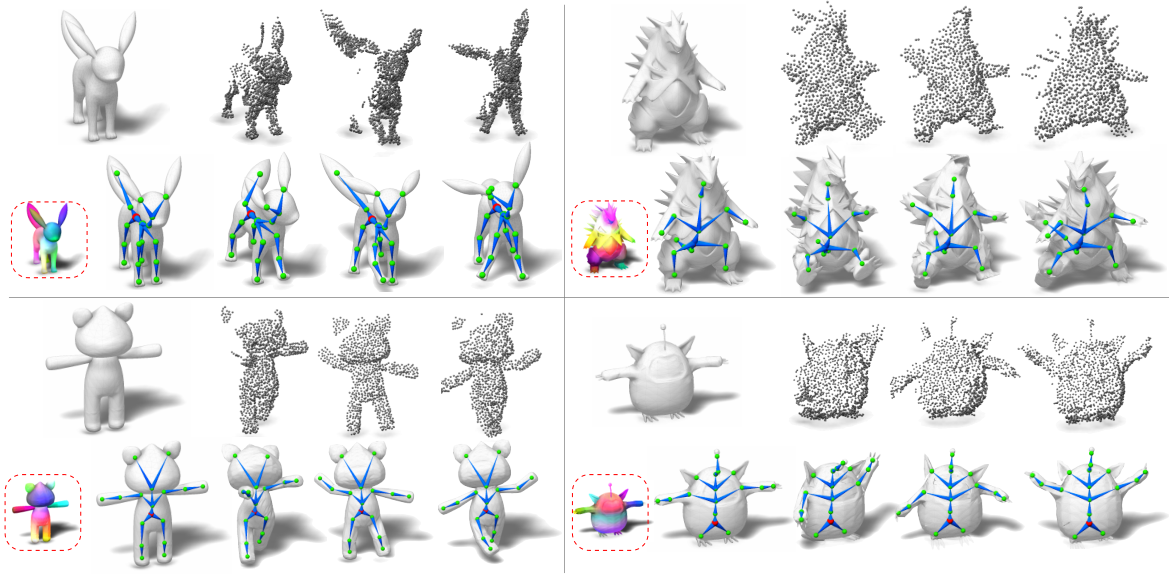
Figure 6 shows four examples of rigging and deformation results from the ModelsResource dataset. The bottom row of Figure 1 shows an additional result of a test quadruped rigged and animated by motion from the DeformingThing4D dataset (not included in our training). For animation results, please see our supplementary video (https://youtu.be/sPxfnQ8j07Y).

Real-world scans.
We also evaluated MoRig’s rigging and animation performance on test cases involving real-world scans. The top row of Figure 1 shows a fictional character rigged and animated using a real-world point cloud sequence from DFaust (Bogo et al. 2017). The top row of Figure 7 shows two more real-world point cloud sequences from DFaust along with resulting rigs and animated meshes from MoRig. The bottom row of Figure 7 shows MoRig’s result driven by two real-world point cloud sequences from KillingFusion (Slavcheva et al. 2017). These scans are noisy and partial, with points accessible only from a single viewpoint, making the problem challenging. Even if our method was not trained on real-world point clouds, our method can still create skeletons capturing the articulated parts in these characters. Quantitatively we evaluate the joints in our rigs compared to animator-created ones for the meshes used in these real-world test cases in Table 2. We also provide the results of RigNet as a comparison. The results show better joint localization compared to RigNet with trends similar to our evaluation on synthetic data. The animated results are shown in the video (3:05-end).
| IoU | Precision | Recall | Chamfer | |
| RigNet | 46.7% | 44.5% | 49.9% | 3.3% |
| MoRig | 65.7% | 70.0% | 62.2% | 3.1% |
Ablation study.

We include comparisons with two alternative variants to produce motion-aware features. Instead of a transformer encoder, we can alternatively produce features by mean or max pooling over the features (see Section 3.3). Our transformer-based encoder yields the best results, as shown in Table 1. We also performed another ablation study to evaluate MoRig’s performance wrt the number of input frames, or poses. In Figure 8, we show the Euclidean distance error between ground-truth vertex positions and predicted ones (as ‘y-axis’) versus number of input poses (as ‘x-axis’). With more frames as input to our motion encoder, the performance is improved since the features become increasingly informative about the articulated parts in the motion.
6. Discussion
We presented MoRig, a method for rigging and animating a character mesh driven by a point cloud sequence of a captured character. Comparing to existing single mesh rigging approaches, our method takes as input an additional point cloud motion sequence, and encodes it into motion features via a deep neural network. The encoded motion features are informative about articulated parts of the target character and thus can achieve more accurate skeletal rigging results.
Our method has limitations that can inspire future research. We assumed that the reference and target character have similar underlying articulation structure. If a part is not visible in an input sequence (e.g., tail), our method will be entirely based on geometry instead of motion and may fail to create a bone for this part. Although we attempted to make our method robust to occlusions and mismatches between part proportions of the target and reference character, large changes in geometry and poses may result in inaccurate rigs and motion transfers. In particular, if the initial point cloud frame is corrupt, then the initial deformation becomes unreliable, and our method will fail. Our method is limited to linear blend skinning, and cannot deal with topological changes. Finally, it requires guidance in the form of point clouds, which may not always easy to capture.
Acknowledgements.
We thank Kentaro Ko, Takuya Narihira, Tamaki Kojima for helpful discussion. We are grateful for the support from Sony Corporation.References
- (1)
- Allen et al. (2003) Brett Allen, Brian Curless, and Zoran Popović. 2003. The Space of Human Body Shapes: Reconstruction and Parameterization from Range Scans. ACM TOG 22, 3 (2003).
- Au et al. (2008) Oscar Kin-Chung Au, Chiew-Lan Tai, Hung-Kuo Chu, Daniel Cohen-Or, and Tong-Yee Lee. 2008. Skeleton Extraction by Mesh Contraction. ACM TOG 27, 3 (2008).
- Avril et al. (2016) Quentin Avril, Donya Ghafourzadeh, Srinivasan Ramachandran, Sahel Fallahdoust, Sarah Ribet, Olivier Dionne, Martin de Lasa, and Eric Paquette. 2016. Animation Setup Transfer for 3D Characters. Comput. Graph. Forum 35, 2 (2016).
- Baran and Popović (2007) Ilya Baran and Jovan Popović. 2007. Automatic Rigging and Animation of 3D Characters. ACM TOG 26, 3 (2007).
- Bogo et al. (2017) Federica Bogo, Javier Romero, Gerard Pons-Moll, and Michael J. Black. 2017. Dynamic FAUST: Registering Human Bodies in Motion. In Proc. CVPR.
- Božič et al. (2021) Aljaž Božič, Pablo Palafox, Michael Zollhöfer, Justus Thies, Angela Dai, and Matthias Nießner. 2021. Neural Deformation Graphs for Globally-consistent Non-rigid Reconstruction. In Proc. CVPR.
- De Aguiar et al. (2008) Edilson De Aguiar, Christian Theobalt, Sebastian Thrun, and Hans-Peter Seidel. 2008. Automatic Conversion of Mesh Animations into Skeleton-based Animations. Comput. Graph. Forum 27, 2 (2008).
- Dionne and de Lasa (2013) Olivier Dionne and Martin de Lasa. 2013. Geodesic Voxel Binding for Production Character Meshes. In Proc. SCA.
- Dosovitskiy et al. (2021) Alexey Dosovitskiy, Lucas Beyer, Alexander Kolesnikov, Dirk Weissenborn, Xiaohua Zhai, Thomas Unterthiner, Mostafa Dehghani, Matthias Minderer, Georg Heigold, Sylvain Gelly, Jakob Uszkoreit, and Neil Houlsby. 2021. An Image is Worth 16x16 Words: Transformers for Image Recognition at Scale. In Proc. ICLR.
- Hayden et al. (2020) David S Hayden, Jason Pacheco, and John W Fisher. 2020. Nonparametric object and parts modeling with lie group dynamics. In Proc. CVPR.
- Huang et al. (2013) Hui Huang, Shihao Wu, Daniel Cohen-Or, Minglun Gong, Hao Zhang, Guiqing Li, and Baoquan Chen. 2013. L1-Medial Skeleton of Point Cloud. ACM TOG 32, 4 (2013).
- Huang et al. (2021) Jiahui Huang, He Wang, Tolga Birdal, Minhyuk Sung, Federica Arrigoni, Shi-Min Hu, and Leonidas Guibas. 2021. MultiBodySync: Multi-Body Segmentation and Motion Estimation via 3D Scan Synchronization. In Proc. CVPR.
- Jacobson et al. (2011) Alec Jacobson, Ilya Baran, Jovan Popoviundefined, and Olga Sorkine. 2011. Bounded Biharmonic Weights for Real-Time Deformation. ACM TOG 30, 4 (2011).
- James and Twigg (2005) Doug L. James and Christopher D. Twigg. 2005. Skinning Mesh Animations. ACM TOG 24, 3 (2005).
- Kavan et al. (2007) Ladislav Kavan, Steven Collins, Jiří Žára, and Carol O’Sullivan. 2007. Skinning with Dual Quaternions. In Proc. I3D.
- Kavan et al. (2010) L. Kavan, P.-P. Sloan, and C. O’Sullivan. 2010. Fast and Efficient Skinning of Animated Meshes. Comput. Graph. Forum 29, 2 (2010), 327–336.
- Kingma and Ba (2015) Diederick P Kingma and Jimmy Ba. 2015. Adam: A method for stochastic optimization. In Proc. ICLR.
- Le and Deng (2012) Binh Huy Le and Zhigang Deng. 2012. Smooth Skinning Decomposition with Rigid Bones. ACM TOG 31, 6 (2012).
- Le and Deng (2014) Binh Huy Le and Zhigang Deng. 2014. Robust and accurate skeletal rigging from mesh sequences. ACM TOG 33, 4 (2014).
- Le and Hodgins (2016) Binh Huy Le and Jessica K. Hodgins. 2016. Real-Time Skeletal Skinning with Optimized Centers of Rotation. ACM TOG 35, 4 (2016).
- Lee and Shin (1999) Jehee Lee and Sung Yong Shin. 1999. A Hierarchical Approach to Interactive Motion Editing for Human-like Figures. In Proc. ACM SIGGRAPH.
- Li et al. (2016) Hao Li, Guowei Wan, Honghua Li, Andrei Sharf, Kai Xu, and Baoquan Chen. 2016. Mobility fitting using 4d ransac. Comput. Graph. Forum 35, 5 (2016).
- Li et al. (2021a) Peizhuo Li, Kfir Aberman, Rana Hanocka, Libin Liu, Olga Sorkine-Hornung, and Baoquan Chen. 2021a. Learning Skeletal Articulations with Neural Blend Shapes. ACM TOG 40, 4 (2021).
- Li et al. (2007) Ting Li, Vinutha Kallem, Dheeraj Singaraju, and René Vidal. 2007. Projective factorization of multiple rigid-body motions. In Proc. CVPR.
- Li et al. (2021b) Yang Li, Hikari Takehara, Takafumi Taketomi, Bo Zheng, and Matthias Nießner. 2021b. 4dcomplete: Non-rigid motion estimation beyond the observable surface. In Proc. ICCV.
- Liu et al. (2019) Lijuan Liu, Youyi Zheng, Di Tang, Yi Yuan, Changjie Fan, and Kun Zhou. 2019. NeuroSkinning: Automatic Skin Binding for Production Characters with Deep Graph Networks. ACM TOG 38, 4 (2019).
- Lu et al. (2018) Xuequan Lu, Honghua Chen, Sai-Kit Yeung, Zhigang Deng, and Wenzhi Chen. 2018. Unsupervised articulated skeleton extraction from point set sequences captured by a single depth camera. In Proc. AAAI.
- Lu et al. (2019) Xuequan Lu, Zhigang Deng, Jun Luo, Wenzhi Chen, Sai-Kit Yeung, and Ying He. 2019. 3D articulated skeleton extraction using a single consumer-grade depth camera. Comput. Vis. Image Underst. 188 (2019).
- Oord et al. (2018) Aaron van den Oord, Yazhe Li, and Oriol Vinyals. 2018. Representation learning with contrastive predictive coding. arXiv preprint arXiv:1807.03748 (2018).
- Parent (2012) Rick Parent. 2012. Computer animation: algorithms and techniques. Newnes.
- Paszke et al. (2019) Adam Paszke, Sam Gross, Francisco Massa, Adam Lerer, James Bradbury, Gregory Chanan, Trevor Killeen, Zeming Lin, Natalia Gimelshein, Luca Antiga, Alban Desmaison, Andreas Kopf, Edward Yang, Zachary DeVito, Martin Raison, Alykhan Tejani, Sasank Chilamkurthy, Benoit Steiner, Lu Fang, Junjie Bai, and Soumith Chintala. 2019. PyTorch: An Imperative Style, High-Performance Deep Learning Library. In Advances in Neural Information Processing Systems 32, H. Wallach, H. Larochelle, A. Beygelzimer, F. d'Alché-Buc, E. Fox, and R. Garnett (Eds.).
- Qi et al. (2017) Charles Ruizhongtai Qi, Li Yi, Hao Su, and Leonidas J Guibas. 2017. Pointnet++: Deep hierarchical feature learning on point sets in a metric space. In Proc. NeurIPS.
- Radford et al. (2021) Alec Radford, Jong Wook Kim, Chris Hallacy, Aditya Ramesh, Gabriel Goh, Sandhini Agarwal, Girish Sastry, Amanda Askell, Pamela Mishkin, Jack Clark, et al. 2021. Learning transferable visual models from natural language supervision. In Proc. ICML.
- Slavcheva et al. (2017) M. Slavcheva, M. Baust, D. Cremers, and S. Ilic. 2017. KillingFusion: Non-rigid 3D Reconstruction without Correspondences. In Proc. CVPR.
- Tagliasacchi et al. (2012) Andrea Tagliasacchi, Ibraheem Alhashim, Matt Olson, and Hao Zhang. 2012. Mean Curvature Skeletons. Comput. Graph. Forum 31, 5 (2012).
- Tzionas and Gall (2016) Dimitrios Tzionas and Juergen Gall. 2016. Reconstructing Articulated Rigged Models from RGB-D Videos. In ECCV Workshops on Recovering 6D Object Pose.
- Vaswani et al. (2017) Ashish Vaswani, Noam Shazeer, Niki Parmar, Jakob Uszkoreit, Llion Jones, Aidan N Gomez, Lukasz Kaiser, and Illia Polosukhin. 2017. Attention is all you need. In Proc. NeurIPS.
- Wang et al. (2019) Xiaogang Wang, Bin Zhou, Yahao Shi, Xiaowu Chen, Qinping Zhao, and Kai Xu. 2019. Shape2Motion: Joint Analysis of Motion Parts and Attributes From 3D Shapes. In Proc. CVPR.
- Xu et al. (2019a) Xun Xu, Loong-Fah Cheong, and Zhuwen Li. 2019a. 3d rigid motion segmentation with mixed and unknown number of models. IEEE TPAMI 43, 1 (2019).
- Xu et al. (2020) Zhan Xu, Yang Zhou, Evangelos Kalogerakis, Chris Landreth, and Karan Singh. 2020. RigNet: Neural Rigging for Articulated Characters. ACM TOG 39, 4 (2020).
- Xu et al. (2019b) Zhan Xu, Yang Zhou, Evangelos Kalogerakis, and Karan Singh. 2019b. Predicting Animation Skeletons for 3D Articulated Models via Volumetric Nets. In Proc. 3DV.
- Yan et al. (2019) Zihao Yan, Ruizhen Hu, Xingguang Yan, Luanmin Chen, Oliver van Kaick, Hao Zhang, and Hui Huang. 2019. RPM-Net: Recurrent Prediction of Motion and Parts from Point Cloud. ACM TOG 38, 6 (2019).
- Yi et al. (2018) Li Yi, Haibin Huang, Difan Liu, Evangelos Kalogerakis, Hao Su, and Leonidas Guibas. 2018. Deep Part Induction from Articulated Object Pairs. ACM TOG 37, 6 (2018).
- Yuan et al. (2016) Qing Yuan, Guiqing Li, Kai Xu, Xudong Chen, and Hui Huang. 2016. Space-Time Co-Segmentation of Articulated Point Cloud Sequences. Comput. Graph. Forum 35, 2 (2016).
- Zhang et al. (2013) Quanshi Zhang, Xuan Song, Xiaowei Shao, Ryosuke Shibasaki, and Huijing Zhao. 2013. Unsupervised Skeleton Extraction and Motion Capture from 3D Deformable Matching. Neurocomputing 100 (2013).
| Layer | Input | Output |
| Point Feature Extractor | ||
| SA(0.5, 0.12, [3, 32, 32,64], 64) | x0: (N, 3) | (N/2, 64) |
| SA(0.25, 0.25, [64+3, 64, 64, 128], 64) | (N/2, 64) | (N/8, 128) |
| SA(0.25, 0.5, [128+3, 256, 256, 256], 64) | (N/8, 128) | (N/32, 256) |
| GlobalSA([256+3, 256, 256, 512]) | (N/32, 256) | (1, 512) |
| FP([512+256, 256, 256]) | (1, 512) | (N/32, 256) |
| FP([256+128, 256, 128]) | (N/32, 256) | (N/8, 128) |
| FP([128+64, 128, 64]) | (N/8, 128) | (N/2, 64) |
| FP([64, 64, 64]) | (N/2, 64) | (N, 64) |
| MLP([64, 64]) + Lin(64, 64) | (N, 64) | (N, 64) |
| Vertex Feature Extractor | ||
| GCU(3, 32) | (M, 3) | x1: (M, 32) |
| GCU(32, 64) | (M, 32) | x2: (M, 64) |
| GCU(64, 256) | (M, 64) | x3: (M, 256) |
| GCU(256, 512) | (M, 256) | x4: (M, 512) |
| MLP([864, 1024]) | cat(x1,x2,x3,x4) | (M, 1024) |
| MaxPool + repeat | (M, 1024) | xg: (M, 1024) |
| MLP([1891, 1024, 256]) + Lin(256, 64) | cat(x0,x1,x2,x3,x4, xg) | (M, 64) |
| Layer | Input | Output |
| GCU(7, 128) | x0: (M, 7) | x1: (M, 128) |
| GCU(128, 256) | (M, 128) | x2: (M, 256) |
| GCU(256, 512) | (M, 256) | x3: (M, 512) |
| MLP([896, 1024]) | cat(x1,x2,x3) | (M, 1024) |
| MaxPool+repeat | (M, 1024) | xg: (M, 1024) |
| MLP([1927, 1024, 256])+Lin(256, 3) | cat(x0, x1,x2,x3,x4, xg) | (M, 3) |
| Layer | Input | Output |
| GCU(6, 64) | x0: (M, 6) | x1: (M, 64) |
| GCU(64, 256) | (M, 64) | x2: (M, 256) |
| GCU(256, 512) | (M, 256) | x3: (M, 512) |
| MLP([832, 1024]) | cat(x1,x2,x3) | (M, 1024) |
| MaxPool+repeat | (M, 1024) | xg: (M, 1024) |
| MLP([1862, 1024, 256])+Lin(256, 32) | cat(x0, x1,x2,x3,x4, xg) | (M, 32) |
| , , : Lin(32, 64) | (M, T, 32) | (M, T, 64) |
| : Lin(64n_head, 64) | (M, T, 64n_head ) | (M, T, 64) |
| MLP([64, 512]) + Lin(512, 32) | (M, T[token], 64) | (M, 32) |
Appendix A Implementation details
The proposed method is implemented in PyTorch (Paszke et al. 2019). Training follows a stage-wise procedure. First, we apply the loss and in the main paper to train the correspondence module on the ModelsResource dataset using the Adam optimizer (Kingma and Ba 2015). We then add the loss to train the deformation module also on the same split. We then fine tune both modules on realistic motion sequences from the DeformThings4D dataset. Next, we train the motion encoder and rigging module together on the ModelsResource dataset with a - mixture of sequences with predicted and ground-truth deformations respectively. We found that using this mixture improves the final performance as it helps the network utilize motion information while maintaining robustness to noises. In all cases, hyperparameters are tuned in the validation splits of these datasets. Training takes about on a Nvidia RTX 8000 for all modules on both training datasets. We provide the network architecture details of the proposed correspondence module, deformation module and motion encoder in Table 3, 4 and 5 respectively along with the corresponding input and output feature sizes.
Appendix B Correspondence Visualizations
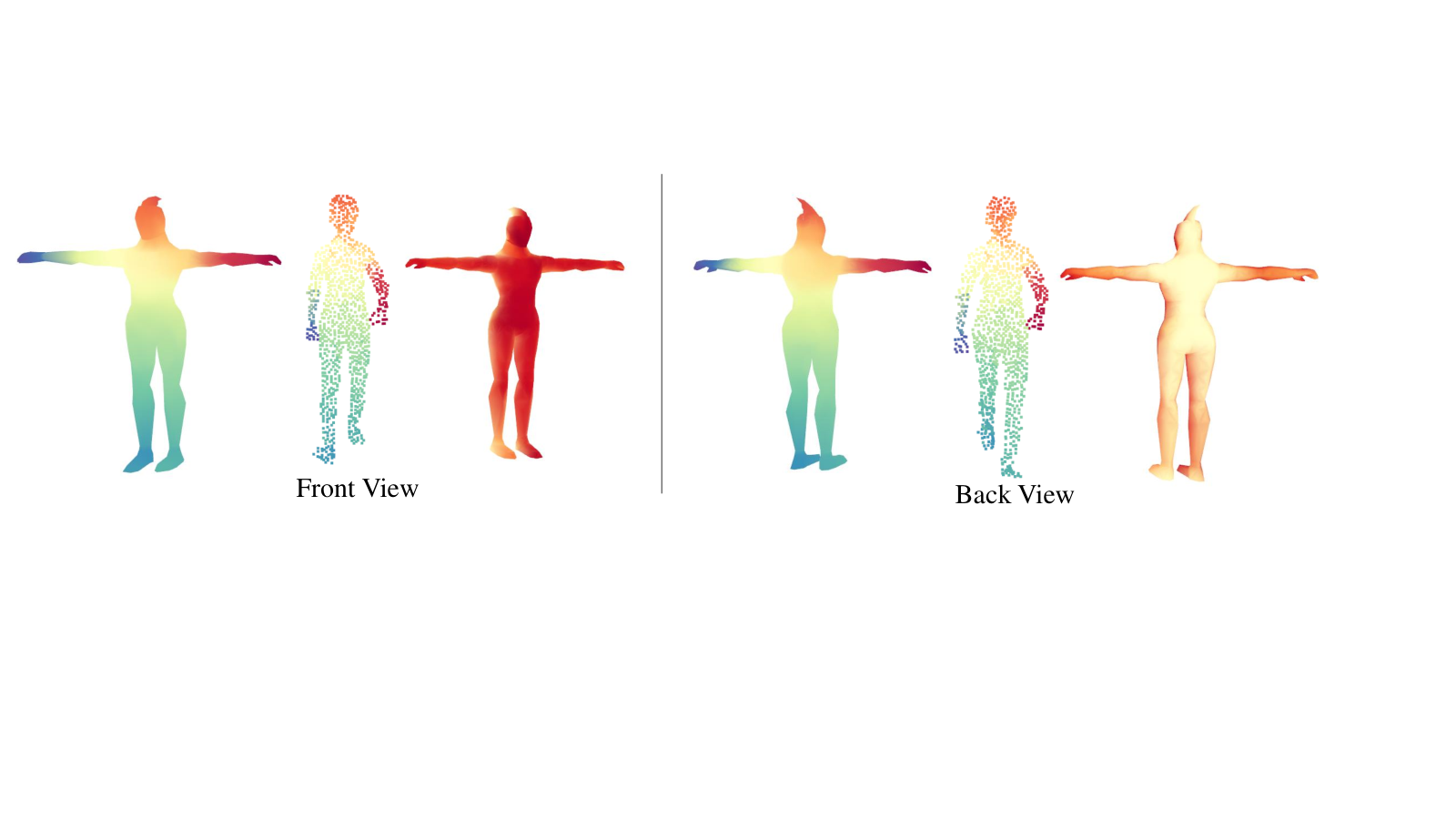
Figure 9 visualizes an example of predicted correspondences between a mesh and a point cloud, as derived from the matching scores and correspondence mask. We show the result from both front and back views. Vertices are color-coded according to their positions, and point colors are determined based on their predicted corresponding vertex. In the correspondence mask, redder color indicates the vertices are more likely to have a corresponding point.