Einstein-scalar field solutions in AdS spacetime: clouds, boundary conditions, and scalar multipoles
Abstract
We consider an Einstein-scalar field model which is a consistent truncation of gauged supergravity, the scalar field possessing a potential which is unbounded from below and a tachyonic mass above the Breitenlohner-Freedman bound. We investigate the spherically symmetric asymptotically anti-de Sitter soliton and black hole solutions, with the aim of clarifying the asymptotics and the possible boundary conditions at infinity. The emerging picture is contrasted with that found for an Einstein-scalar field model with the same scalar mass and a quartic self-interaction term. We also provide arguments for the existence of solitonic solutions which can be viewed as non-linear continuation of the (probe) scalar multipolar clouds, with emphasis on the dipole case. Apart from numerical results, exact solutions are found for solitons with a monopole and dipole scalar field, as perturbations around the AdS background.
1 Introduction
The study of scalar fields in AdS spacetime can be traced back at least to the work Salam:1977hk, Avis:1977yn, where the massive Klein-Gordon equation has been solved in an AdS4 background. More recently, this subject has been of particular interest mainly due to the AdS/CFT duality Maldacena:1997re, which asserts that a consistent theory of quantum gravity in -dimensions has an equivalent formulation in terms of a non-gravitational theory in -dimensions.
One well understood limit of the duality is when, in the AdS bulk, it is sufficient to consider the low energy limit of the superstring theory, namely, supergravity (for a review, see Ref. Aharony:1999ti). The supergravity models usually contain tachyonic scalar fields and, in some cases, there exist consistent truncations such that the matter content consists only of scalar fields. The solutions of these models are particularly interesting due to non-trivial boundary conditions satisfied by the scalar field(s) Hertog:2004ns that are relevant for the dual theory Witten:2001ua. For example, the scalar fields can break the conformal symmetry on the boundary Henneaux:2006hk, and exact hairy black hole (BH) solutions with this property were presented in Lu:2013ura. Also, the lowest energy solitonic solutions can be considered the true ground state of the theory Hertog:2004ns, Hertog:2005hm, while the study of the thermodynamic properties of AdS BHs offers the possibility to better understand the non-perturbative aspects of certain dual field theories.
Of interest in this context is the gauged supergravity model that can be obtained as a compactification of supergravity on deWit:1986oxb. As discussed in Duff:1999gh (see also Cvetic:1999xp and Gibbons:2005vp), this model possesses a consistent truncation with three real scalar fields of equal mass, coupled to four U(1) fields, which can be set to zero. The scalar fields can also vanish, a case which results in Einstein gravity with a negative cosmological constant (with the AdS radius). The main solution of interest is the AdS4 spacetime in global coordinates
| (1) |
with the radial and time coordinate, respectively, while are the usual coordinates on . Otherwise, as discussed in Appendix A, we can (consistently) take only one scalar field to be nonzero (), or two of them () (in which case, they are equal); finally, all scalars can be taken nonzero and equal, , the resulting Einstein-(single, real) scalar field model being presented in Section 2. For any nonzero , the scalar field possess a tachyonic mass .
In this work, we are interested in static and localized solutions of the considered Einstein-scalar field model, which are also regular and have a finite mass. They may possess an event horizon of spherical topology (and then correspond to BHs with scalar hair) or just correspond to solitonic deformations of the globally AdS spacetime (1). In both cases, the generic expression of the (static) scalar field as (which is found by considering the linearized Klein-Gordon equation in a fixed AdS background) is the sum of two modes
| (2) |
and being two real functions. For a well defined theory, one has to specify a boundary condition on , the natural choice corresponding to either or . However, as shown in Hertog:2004ns Henneaux:2002wm, Henneaux:2004zi, Hertog:2004dr, one may consider a larger class of mixed boundary conditions, with nonzero and , for which the conserved global charges are still well defined and finite. The boundary conditions in this case are defined by an essentially arbitrary function connecting and , with
| (3) |
Since their properties depend significantly on the choice of , this type of models have been called designer gravity theories Hertog:2004ns.
The expressions of and are not determined a priori, various boundary conditions being possible, that lead to different properties of the solutions. Also, and in the large- expansion (2) are not arbitrary, being determined by the imposed data at the origin (for solitons), or at the horizon (for BHs). For example, a priori one expects the existence of solutions with or . However, to our best of knowledge, no systematic study of this aspect has been presented in the literature. For , we mention the study in Refs. Hertog:2004dr, Hertog:2004rz, Hertog:2004bb, where spherically symmetric solutions with are studied (with a negative constant).
The first goal of the present work is to consider a systematic study of the spherically symmetric solitonic and BH solutions of the considered consistent truncation of the model. The aim is to clarify the dependence of the data at infinity on the data at the origin/horizon,
| (4) |
(with or for solitons and BHs, while is an extra-constant which enters the far field expression of the metric), without imposing any relation between and .11 1 A similar analysis in five dimensions, but with a different goal, was presented in Anabalon:2017eri. The main results can be summarized as follows. Firstly, both perturbative and non-perturbative solutions are considered. The perturbative results are found for solitons, the perturbation parameter being , the value of the scalar field at the origin. The non-perturbative solutions are found by solving numerically the field equations, in which case we aim for a systematic scan of the parameter space for a large range of . Secondly, our results provide strong evidence for the of (soliton or BH) solutions satisfying the ‘standard’ conditions or . That is, the model possesses designer gravity solutions only.
A natural question which arises in this context concerns the generality of these results. In particular, is it possible to find solutions with or in (2) for a different choice of the scalar field potential? To address this aspect, we study also solutions of a model in which the scalar field still possesses the same mass as in the case; however, the self-interaction is given by a quartic term. As a result, the asymptotic behaviour of the scalar field is less constrained and one finds spherically symmetric solutions with or in the expansion (2).
Another goal of this work is motivated by the observation that, to our best knowledge, all Einstein-(real) scalar field solutions reported in the literature correspond to spherically symmetric configurations. However, the (static) solution of the linearized Klein-Gordon equation in a fixed AdS background possesses a general solution, the scalar field being a superposition of modes, (with the real spherical harmonics and the radial amplitude). From this perspective, no value of is privileged, with the same asymptotic decay (2) for all modes (see, also, Horowitz:2000fm). Also, since the spherically symmetric Einstein-scalar field solitons can be viewed as a non-linear continuation of the mode, one expects similar results to exist for higher modes. In this work we consider mainly the simplest case and we provide evidence that the qualitative picture found in the spherically symmetric case still holds. First, one finds again an exact, perturbative solitonic solution, which is interpreted as a deformation of AdS spacetime with a dipolar scalar field. Nonperturbative solutions with a -decay at infinity of the scalar field are shown to exist in a model -selfinteraction.
This paper is organized as follows. In the next Section we present the general framework, while in Section 3 we consider the probe limit of the problem, with a study of scalar clouds in a fixed (Schwarzschild-)AdS background. The case of spherically symmetric configurations is discussed in Section 4, while the gravitating scalar dipoles are studied in Section 5. We conclude in Section 6 with a discussion and some further remarks. The Appendix A explains how the considered sugra-action is obtained starting with the general results in Ref. Duff:1999gh. In the Appendix B, we provide some details on the perturbative axially symmetric solutions, including the Einstein-scalar field soliton with a quadrupole scalar field.
2 The general framework
2.1 The action, equations of motion and scalar field potentials
We consider the Einstein-(real)scalar field model with a negative cosmological constant
| (5) |
where (with the Newton’s constant) and is the scalar field potential. Also, the last term in (5) is the Hawking-Gibbons surface term Gibbons:1976ue, where is the trace of the extrinsic curvature for the boundary and is the induced metric of the boundary.
The corresponding Einstein-scalar field field equations, as obtained from the variation of the action (5) with respect to the metric and scalar field, respectively, read:
| (6) |
where is the stress-energy tensor of the scalar field,
| (7) |
In this work we shall consider two different expressions of the scalar field potential . The first case is of main interest, occurring in a consistent trucation of the gauged supergravity model deWit:1986oxb, with
| (8) |
The Appendix A presents some details on how the action (5) with the above potential can be obtained starting with the general results in Ref. Duff:1999gh.
2.2 Mixed boundary conditions and holographic mass
In this section we present a general discussion of possible boundary conditions for a scalar field with the tachyonic mass (10), the interpretation within AdS/CFT duality, and a concrete method to obtain the holographic mass. We are going to follow closely the Refs. Marolf:2006nd and Anabalon:2015xvl, where counterterms for the scalar fields were used to regularize the action and to obtain the holographic mass. These results can be directly applied to various examples considered in the next sections.
While in theories of gravity coupled to matter the theory is usually fully determined by the action, in the presence of scalar fields with tachyonic mass the situation is quite different. That is, both modes in the scalar field’s fall off (2) are normalizable and represent physically acceptable fluctuations. Therefore, specifying boundary conditions for the scalar field is equivalent to fixing the boundary data , or a specific relation between them. It is common to denote the mixed boundary conditions on the scalar field by , where is an arbitrary differentiable function. This restriction on and can be obtained from the vanishing symplectic flux flow through the boundary Amsel:2006uf and it is interpreted as an integrability condition for the mass in the Hamiltonian formalism Hertog:2004ns, Anabalon:2014fla.
The existence of various boundary conditions for the scalar fields fits very well in the context of AdS/CFT duality where they are interpreted as multitrace deformations in the dual field theory Witten:2001ua. The interpretation is as follows: if is identified with the source for an operator in the dual field theory, , the dual field theory action should contain a term and then is identified with the vacuum expectation value (VEV) of the operator, (and the other way around with the source and the VEV). However, for the current work, the mixed boundary condition, , is the relevant one with the following interpretation: these general boundary conditions are multitrace deformations of the boundary CFT, of the form . A generic deformation can break the conformal symmetry in the boundary, but since it is still invariant under global time translations, there exists a conserved total mass/energy. As we are going to explicitly show below, the mixed boundary conditions that preserve the conformal symmetry can be obtained from the vanishing trace of the dual stress tensor and correspond to triple trace deformations.
After this brief review of mixed boundary conditions for the scalar field and their interpretation within the AdS/CFT duality, let us obtain the holographic mass by using the ‘counterterm method’, that consists in adding suitable additional surface terms to regularize the action (5). These counterterms are usually built up with curvature invariants on the boundary (which is sent to infinity after the integration); as such, they do not alter the bulk equations of motion. In four spacetime dimensions, the following counterterms are sufficient to cancel divergences for (electro-)vacuum solutions with negative cosmological constant Henningson:1998gx, Balasubramanian:1999re, Skenderis:2000in
| (12) |
where is the Ricci scalar of the boundary metric . Within this approach, the mass computation goes as follows. First step consists in constructing a divergence-free boundary stress tensor from the total action by defining
| (13) |
where is the Einstein tensor of the boundary metric, is the extrinsic curvature, being an outward pointing normal vector to the boundary. Here one supposes that the boundary geometry is foliated by spacelike surfaces with metric
| (14) |
Then, if is a Killing vector generating an isometry of the boundary geometry, there should be an associated conserved charge. In this approach, is the proper energy density while is a timelike unit vector normal to . Thus the conserved charge associated with time translation is the mass of the spacetime
| (15) |
The presence of the scalar field in the bulk action (5) brings the potential danger of having divergent contributions coming from both, the gravitational and matter actions Taylor-Robinson:2000xw. This is the case for a scalar field which behaves asymptotically as ( in (2)), and then the counterterms (12) will not yield a finite mass. However, it is still possible to obtain a finite mass by allowing the boundary counterterms to depend not only on the boundary metric , but also on the scalar field. This means that the quasilocal stress-energy tensor (13) also acquires a contribution coming from the matter field. The counterterm that regularizes the action and has a valid variational principle compatible with the boundary condition is Anabalon:2015xvl
| (16) |
that yields a supplementary contribution to the boundary stress tensor (13),
| (17) |
which should be taken into account when obtaining a finite mass, eq. (15).
We also mention that the background metric upon which the dual field theory resides is (with the radial coordinate). Then, the expectation value of the dual CFT stress-tensor can be calculated using the relation Myers:1999qn
| (18) |
with the trace Anabalon:2015xvl
| (19) |
It follows that the only mixed boundary condition, which preserves the conformal symmetry corresponds to a triple trace deformation in dual field theory, . In this case, the trace of the dual stress tensor vanishes.
In this approach, given some data at infinity , one can assign a well defined mass only after defining the function , eq. (3). In principle, this result can be circumvented by using the counterterm in Refs. Lu:2013ura, Gegenberg:2003jr, Radu:2004xp,
| (20) |
which does not require to specify a condition for and . However, this counterterm is problematic because it is not intrinsic to the boundary and also, for mixed boundary conditions, the variational principle is not satisfied. Moreover, it implies generically a vanishing trace of the boundary stress tensor (although for the mass expression coincides with that found using (17)).
2.3 Remarks on numerics
While it was possible to find some partial analytical results, the non-perturbative solutions are constructed numerically, by integrating the system of Einstein-scalar field equations (6) subject to suitable boundary conditions. Both solitons and BHs will be considered. However, note that in order to simplify the problem, in the BH case we restrict the study to the region outside the event horizon. For spherically symmetric solutions, we use a standard Runge-Kutta ordinary differential equation solver. All numerical calculations in the axially symmetric case have been performed by using a professional package, which uses a Newton-Raphson finite difference method with an arbitrary grid and arbitrary consistency order schoen.
The numerics are done working with a scaled scalar field and a scaled radial coordinate,
| (21) |
that results in the following Lagrangian of the considered models (note that for the case, we supplement (21) with )
| (22) |
with
| (23) |
However, for the sake of clarity, all equations displayed in what follows are given in terms of dimensionful variables.
3 Probe limit: static scalar clouds in AdS
Before considering the full problem, it is interesting to consider first the probe limit, and to study solutions of the Klein-Gordon equation in a fixed geometry, while neglecting the backreaction of the scalar field. The background can be the AdS spacetime or the Schwarzschild-AdS (SAdS) BH, which possesses a line element of the form (1), with22 2 The expression (24) results from the usual SAdS expression, with .
| (24) |
where is the event horizon radius and the BH mass.
This approximation greatly simplifies the problem but retains some of the interesting physics. Both linear ( with a mass term only in the potential ) and non-linear clouds will be considered. In both cases, the mass-energy density of a configuration, as measured by a static observer with velocity , is . Then one can define a total mass of a cloud,
| (25) |
One can see that, in order for to be finite, should decay faster than as . Then, for the scalar field asymptotics (2), the term proportional with should be absent, in the large -limit.
3.1 The linear case
Let us start with the case of a massive scalar field with no self-interaction ( with ) in a fixed AdS background (1), and consider solutions of the (linear) KG equation
| (26) |
The scalar field can be decomposed in a sum of modes
| (27) |
where are the real spherical harmonics (with and ), while the radial amplitude is a solution of the equation
| (28) |
where a prime denotes the derivative the radial coordinate .


For the case of interest in this work with , the general solution of the above equation reads (with the hypergeometric function)
| (29) | |||||
being the sum of two modes (with arbitrary constants). However, the second term in the above relation diverges as and thus we set (also, in what follows, we take ). The explicit form of the solution for the first three values of reads


| (30) |
the expressions for higher becoming increasingly complicated.
As , the (regular) solution has the following form
| (31) |
As spatial infinity is approached, all multipoles decay according to (2), such that the approximate form of a -mode reads
where
This behaviour strongly contrasts with that found for a Minkowski spacetime background, where the scalar mode which is regular at diverges as This feature can be traced back to the “box"-like behaviour of the AdS spacetime, and is present also for a Maxwell field Herdeiro:2015vaa.
The above solution contains already several features that will also be found in the (self-gravitating) sugra-case. First, one notices that all multipoles share the same far field decay. Second, the radial amplitude is always nodeless. Moreover, both parameters and are non-zero. As such, the linear cloud mass, as computed according to (25) diverges, although the energy density is finite everywhere.
One may ask if the situation is different when considering a SAdS BH background. Although no exact solutions of the radial equation appear to exist, the eq. (28) can be solved numerically. The approximate expansion of the radial amplitude as reads
| (32) |
while the asymptotic expansion of a mode is given by (2), with
| (33) |
where the constants depend on the value of .
As seen in Figure 1, the presence of a horizon does not change the picture found for solitons. In particular, there are no scalar clouds33 3 The apparent divergence for of , as is an artifact of solving the (linear) equation (28) with the boundary condition , while in the solitonic limit. with or .


3.2 Non-linear clouds in the model
One may inquire how general are the above results and what are the new results induced by the scalar field self-interaction. In particular, are there scalar clouds with (which then would possess a finite mass)?
While the picture found for the sugra-potential (8) appears to be qualitatively similar to that found for linear clouds (and we could not find solutions with ), the situation is different for a model with a quartic self-intercation. An indication in this direction44 4 An exact solution with and a finite mass is found in a model with a cubic-selfinteraction (34) as provided by the existence of the following exact solution55 5 Note that the solution with real exists for only. describing a spherically symmetric soliton in the -model:
| (35) |
We have studied generalizations of this exact solution, by solving numerically the scalar field equation for a (S)AdS background and varying (the value of the scalar field at the horizon or the origin, , for the soliton), the values of the parameters and being extracted from the numerical output. In the numerics, we set without any loss of generality, via a suitable scaling of the scalar field.
Some numerical results are shown in Figure 2 where one can observe that the parameters and can be zero, for a (presumably infinite) set of discrete values of . For example, in the solitonic case (), the exact solution (3.2) corresponds to , while the first configuration with is found for (which strongly suggests the existence of an exact solution also in that case). Moreover, for the solutions possess at least a node.
In Figure 3 (left panel) we present a number of relevant quantities as a function of the horizon radius for the subset of (finite mass) solutions with . As one can see, no restrictions seem to exist on the BH size, while for large enough BHs, both and increase linearly with .
Since one has to solve numerically a (nonlinear) partial differential equation (PDE), the case of higher multipoles is technically more complicated. Restricting to axisymmetric configurations, this is a particular case of the problem discussed in Section 3, being solved by using a similar numerical approach. Moreover, we have mainly studied the case of finite mass dipoles66 6 However, we have confirmed the existence of similar solutions also for quadrupoles. with in the scalar far field expansion, the decay being imposed by introducing a new function , and requiring as . Other boundary conditions satisfied by the scalar field are at and at , while the field is (still) odd-parity, In Figure 4 (left panel) we display the profile of the AdS dipole solution, which possesses a finite mass . We note that the extrema of the field are located on the axis (with ) and are symmetric the equatorial plane.
We shall also mention that the labeling of the solutions in terms of multipoles is ambiguous in a non-linear setup, since the ‘pure-cloud’ feature of the linear solutions is lost due to self-interaction. As such, stands rather for the number of angular nodes of the scalar profiles (with for spherical solutions, for dipoles (one node at ), etc). For example, for a dipole solution, one can write the following expansion of the scalar field
| (36) |
with the Legendre polynomials. Although the term dominates, the contribution of the higher order terms is also nontrivial, as can be seen already in the profile of the function (in the right panel of Figure 4). While for a linear cloud , this is not the case when there exists a nonzero contribution of higher order -terms.
As expected, similar solutions are found (numerically) in the presence of a BH horizon, for a SAdS background. The numerics is done in terms of a new radial coordinate in the line-element (1), (24), such that the horizon is located at , where we impose (with ). The boundary conditions on the -axis and at infinity are similar to those imposed for . In Figure 3. we have shown the mass of the solutions and the value of as a function of the horizon radius. One can see that the picture is very different as compared to that found in the spherically symmetric case. As for , a branch of solutions (label (1) in Figure 3) smoothly emerges when adding a horizon at the center of a soliton. Along this branch the mass increases, while the maximal value of decreases. However, for , one finds the existence of a maximal value of , with a back bending and the occurrence of a secondary branch of solutions (label (2)), which extends backwards in . As along this secondary branch, , while the mass of the solutions appears to diverge.77 7 This behaviour can be understood by noticing that, for the (scaled) units (21) we employ in numerics, can also be approached as (and thus a vanishing cosmological constant), while the background metric becomes the Schwarzschild BH. However, no smooth solution exists in this case Herdeiro:2015waa.
4 Spherically symmetric Einstein-scalar field solutions
4.1 The Ansatz, equations and asymptotics
The spherically symmetric solutions are constructed by using the following Ansatz for the metric and scalar field
| (37) |
where it is convenient to take
| (38) |
with a mass function. From (6) we find the following equations for the metric functions and the scalar field:
| (39) |
There is also a 2nd order constraint equation
| (40) |
which, however, is a differential consequence of the equations for in (39).
The Ricci scalar and the Kretschmann scalar are given by
| (41) |
For all solutions reported in this work, both and are regular everywhere on the considered domain of integration88 8 Thus, for BHs, this holds on and outside the event horizon..
The system of equations (39) will be solved first perturbatively and then numerically. In both cases, it is useful to find the approximate form of the solutions at the boundaries of the domain of integration.
4.1.1 The small- expansion
Starting with the solitonic case, the small- solution can be written in the form
| (42) |
the series coefficients , , , being determined by the values of the functions and at . No general pattern for these coefficients appears to exist, the first terms being
with , , .
4.1.2 The near-horizon solution
Apart from solitons, we are also interested in BH solutions. They possess a non-extremal horizon99 9 We did not find any indication for the existence of extremal BH solutions. In fact, their absence is also suggested by the absence of an attractor solution with an geometry, which would describe the near horizon of the extremal BHs. located at , where . Close to the horizon, we assume the existence of a power series expansion of the solution in , with
| (43) |
the coefficients being determined by the horizon values of the functions and . One finds
| (44) |
where we denote , , . Also, since the model (22) is invariant when taking , it is enough to consider the case , only (or for solitons).
4.1.3 The large- approximate solution
Finally, the large- approximate expression of the solutions holds for both solitons and BHs. For a generic scalar potential with
| (45) |
an approximate form of the solutions1010 10 Let us remark that the equations of the model are invariant when taking , a symmetry which is lost when imposing can be written as series in , with
| (46) |
with the coefficients depending on the free parameters . One finds, ,
| (47) | |||
where denotes .
Also, the leading order expression of the metric functions and reads
such that the spacetime is still asymptotically (locally) AdS.
4.1.4 Quantities of interest
The Hawking temperature and horizon area of the BH solutions are fixed by the horizon data, with
| (48) |
The mass computation is a straightforward application of the general formalism in Section 2.2. For a given design function (as given by (3)), the non-vanishing components of the resulting boundary stress-tensor are (here we choose to be a three surface of fixed , while ):
Then the mass of these solutions, as computed from (2.2) is
| (49) |
with the function (3) imposing a condition between and .
4.2 Solutions in the model
4.2.1 Perturbative solitons
In the solitonic case, a simple enough exact solution can found perturbatively in terms of the scalar amplitude . The Ansatz for a perturbative approach is:
| (50) |
The solution for the lowest order in is valid for any scalar selfinteraction, since only the mass term is relevant here. One finds
| (51) | |||
where we define the auxiliary functions
| (52) |
Although the equations can be solved to the next order in , the solution with a generic parameter in the potential (8) is exceedingly complicated. Thus in what follows, we shall restrict our study to the special case , where the solution still possesses a simple enough form, with
| (53) |


While , the function is more complicated, with the presence of the poly-logarithm function ,
| (54) |
where


where is the Riemann zeta function1111 11 Note that is a real function, despite the presence of in its expression..
The above expressions allow for a discussion of some basic properties of the solitonic solution. For example, the small- expansion of the scalar field reads
| (55) |
In the context of this work, the coefficients which enter the far field asymptotics are of special interest, with
| (56) | |||
(where we denote ). One notices that is positive and negative to order , which suggests the absence of solutions with and to all orders, a conjecture which is confirmed by the nonperturbative results in the next Subsection. Also, one should remark that are not independent, being parameterized by . The choice of the function (cf. eq. (3)) fixes this parameter; for example, for , while for ).
The expression of the metric potential at the origin (which provides a measure on how strong are the gravity effects) is also of interest, with
| (57) |
Finally, we mention that given a design function (which would fix the parameter ), the mass of the solitons results directly from the eqs. (49), (56).


4.2.2 Nonperturbative results
The nonperturbative solutions are found by integrating numerically the equations (39). In our approach, suitable initial conditions resulting from (42), (43), are imposed at (with for solitons and BHs respectively), for global tolerance , the equations being integrated towards .
In principle, the full set of solutions can be scanned in this way by varying the boundary data at (which is provided by ) and extracting from the numerical output the parameters in the far field, together with .
The profile of a typical soliton solution is shown in Figure 5 for (left panel) and (right panel). Both configurations have the value of the scalar field at the origin, ; however, some features of the solutions depend on the value of (one finds , for and , for ). A similar picture is found for BHs, as shown in Figure 6 for solutions with and (in which case , for and , for ).


Also, for we have included the profile of the perturbative solution with ; as one see, this provides a good approximation of the non-perturbative result. Moreover, the displayed profiles are typical and so far we could not find any indication for the existence of solutions with the function changing sign ( with the existence of nodes).
In Figure 7 we show how the parameters , , and vary with for soliton solutions with1212 12 We have considered as well solutions with and have found that they follow the pattern. . In particular, we remark that is always strictly positive (and increasing with ) while . For , we have included also the corresponding perturbative results. As one can see, they stop to be reliable when becomes around one.
Turning now to BH solutions, we have considered a systematic scan of configurations by varying both and in steps of . The emerging picture is displayed in Figures 8, 9 and can be summarized as follows. First, no configurations with or exist, at least for the considered range of (note, however, the existence of local extrema of these quantities). Second, for any horizon size, both the parameter and the Hawking temperature increase with . Also, we mention that the function decreases monotonically with which makes the study of solutions with large values of the scalar field at the horizon difficult.
Finally, let us remark that the results in Figure 8 imply only rather weak restrictions on the function which connects and in designer gravity theories, since all positive (negative) values of are realized1313 13 For example, the choice imposes only .. In Figure (10) we show the mass of BHs as a function of for several different functions (which corresponds to consider specific slices in the general plots above). As one can see, the minimal value of is achieved in the solitonic limit, with the existence of two solitons for the same value of the scalar field at the horizon. A similar picture has been found for solutions.
4.3 Solutions in the -model
Some of the features above are shared by the gravitating solutions in the -model. For example, a continuum of solutions is found again when varying the values of and (or ), without any indication for the existence of an upper bound for these parameters. As with the sugra case, the generic -solutions have nonzero parameters , . In Figure 10 (right panel) we show the mass of BH solutions with three different choices of the condition . One can notice a (qualitatively) similar picture to that found for solutions with the potential (8).
There are also a number of new specific properties, the most interesting one being that a scalar potential with quartic self-interaction allows for solutions with or in the asymptotic expansion (2).


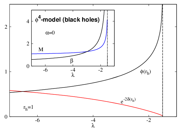

In what follows we shall restrict our study to configurations with , in which case the mass function approaches a constant value at infinity. The profile of two typical solutions are shown in Figure 11 (note that for some range of , such that solutions violate the weak energy conditions). In Figure 12 (left panel) we show how several quantities of interest vary as a function of for -solitons. No solutions with were found for , while our results suggest1414 14 Note that this is smaller than the value found for the truncation of the sugra-potential (8); the absence of configurations with or in the sugra-case can presumably be attributed to the fact that the quartic effective term in the potential (8) never becomes dominant. the existence of a maximal value of , with . As is approached, the function takes very small values close to zero, and the Ricci scalar appears to diverge.
As seen in the left panel of Figure 13, a similar picture is found in the presence of a BH horizon, without the existence of an upper bound on the horizon size (we mention that the same picture was found for other values of ). In Figure 13 (right panel) we show the result for solutions with a fixed value of and a varying horizon size. One can see that the familiar SAdS thermodynamics is recovered for BHs with scalar hair, with the existence of two branches of solutions which join for a minimal value of the Hawking temperature.
5 Beyond spherical symmetry: gravitating scalar dipoles
On general grounds, one expects that each (linear) AdS scalar cloud with given numbers would possess nonlinear continuations in the full Einstein-scalar field model (and thus, the spherically symmetric ( mode) case discussed above is not special). In what follows we present results for the simplest case of (axially symmetric) scalar dipoles (note, however the perturbative construction of the quadrupole solution in the Appendix B). Such configurations are first constructed within a perturbative approach, by considering the backreacting version of the (linear) mode in Section 3.1. Non-perturbative solutions of the Einstein-scalar field equations with a far field decay of the scalar field are constructed in the -model.
5.1 Perturbative results
In constructing perturbatively axially symmetric solutions it is convenient to consider a generalization of the pure line element (1) with three unknown functions ,
| (58) |
with
| (59) |
The scalar field only depends on , with the following perturbative ansatz up to order :
| (60) |
where is a linear scalar on studied in Section 3.1 and is an infinitesimally small parameter. The backreaction of the scalar field on the geometry is taken into account by defining (with )
| (61) |
Then the coupled Einstein–scalar field equations are solved order by order in , the constants which enter the solution being fixed by imposing regularity at and AdS asymptotics.
To illustrate this procedure, let us consider the backreaction on the geometry of a scalar dipole cloud (similar results for the case are given in the Appendix B.3). Thus the lowest order data is
| (62) |
Then, the perturbed metric solution is constructed by considering an angular expansion of in terms of Legendre functions, with coefficients given by radial functions. To lowest order one takes the consistent ansatz
In solving the Einstein equations, one uses a residual gauge freedom to set the radial function , the expressions of the other functions being (we recall )
| (63) | |||
Moving now to the next order in , we shall restrict again to the case in the potential (8). The correction induced by the metric corrections to the scalar field are found by taking a (consistent) ansatz for with two unknown functions,
| (64) |
The explicit form of the functions and is given in the Appendix B.2. In deriving it, we impose them to be regular at and to decay as in . As such, the expansion parameter can be identified with the function (evaluated at ) that enters the far field expansion (2) of the scalar field, and thus
| (65) |
The corresponding expression of is
| (66) |
where we denote
The presence of the term proportional with in the far field expansion of above indicates that, to order , the asymptotic behaviour of the scalar field deviates from that of a dipole.
Different from the spherical case, we were not able to solve the equations to higher order in . However, likely the above solution already captures same basic features of the general configurations. One finds, ,
| (67) |
while the leading order terms in the large- expressions of the metric potentials are
| (68) |
Also, the non-vanishing components of the boundary stress tensor, as computed by using the prescription in Section 2.2 are
| (69) |
Then, to order , the (cubic) term (which is multiplied with the function ) in the scalar counterterm (17) does not show up, and one finds the following simple expression for the mass of the gravitating dipole solution
| (70) |
(where we choose to be a surface at constant , while ).
5.2 Non-perturbative solitons in the -model
5.2.1 The framework
The (axially symmetric) non-perturbative solutions are constructed by employing the Einstein-De Turck approach Headrick:2009pv, Adam:2011dn. Therefore, instead of the Einstein equations, we solve the so called Einstein-DeTurck (EDT) equations
| (71) |
being the Levi-Civita connection associated to the spacetime metric that one wants to determine. Also, a reference metric is introduced, with the corresponding Levi-Civita connection. Solutions to (71) solve the Einstein equations iff everywhere on . To achieve this, we shall impose boundary conditions which are compatible with on the boundary of the domain of integration.
Within this approach, the (static, axially symmetric) metric Ansatz is more complicated than the perturbative one, eq. (58), with five metric functions
For solitons with a decay of the scalar field (the only considered case), the obvious reference metric is AdS spacetime, while the numerics is done with a scalar field Ansatz
| (73) |
such that a vanishing as corresponds to in (2).
Then the EDT equations (71) together with scalar field equation result in a set of six elliptic partial differential equations, which are solved numerically as a boundary value problem. Following the standard approach Dias:2015nua, the boundary conditions are found by constructing an approximate form of the solutions on the boundary of the domain of integration compatible with the requirement . They read
Moreover, we shall assume again that the solutions are symmetric a reflection in the equatorial plane, which implies that the functions satisfy Neumann boundary conditions at while and vanish there. It is also of interest to display the far field behaviour of solution
| (74) | |||
the functions and , , being determined from the numerics.
One finds in this way the following large- expressions of the non-vanishing components of the boundary stress tensor (note the absence of a contribution from the scalar counterterm (17)):
which is traceless, as expected. Then a straightforward computation leads to the following expression for the mass:
5.2.2 Numerical results
In this approach, the only input parameter is , the constant of the quartic self-interaction. Instead of , the numerics is done by using a compactified radial coordinate , the equations being discretized on a () grid with around points. Then the resulting system is solved iteratively until convergence is achieved. The typical numerical error for the solutions reported in this work is estimated to be of the order of (also, the order of the difference formulae was 6).
The profile of the typical scalar field, the function and the energy density are (qualitatively) similar to those displayed in Figure 4 for solutions in the probe limit. As expected, the -(AdS probe) solution with found in Section 3.2 possesses gravitating generalizations. The resulting picture shares the basic features found for spherically symmetric solitons, see Figure 12. The solutions with a decay exist up to a minimal value of (while again no such solutions are found for ). As the minimal value of is approached, both the mass and increase, while the numerics become increasingly challenging, with large numerical errors.
Also, the solutions appear to exist for arbitrary large values of . To understand this limit, one notes that these Einstein-scalar field solutions can also be constructed by using an alternative scaling, with and with an arbitrary nonzero constant. This can be used to set , and work instead with the following form of the EDT equations with . As such, corresponds to solutions in the probe limit (being approached for large values of ).
We mention that the preliminary results indicate the existence of BH generalizations of these solutions, with the presence, as in the probe limit in Section 3.2, of two branches of solutions which merge for a maximal value for the horizon area. However, their study is more involved, being beyond the purposes of this work.
Returning to the solitonic case, such solutions should exist as well for a pure asymptotic decay of the scalar field, or, more generally, with nonzero and in Eq. (2). However, so far we did not manage to adapt our numerical scheme to these cases. The obstacle is that the EDT approach requires the choice of a suitable background metric , which is not obvious for a decay of the scalar field. For example, when choosing AdS for , we could not find a consistent far field expression of the solutions which is compatible with the requirement . This obstacle has also prevented us to find non-perturbative solutions in the model.
We also mention that no results were found when modifying the code used in the -model for a scalar potential given by (8), while keeping the same set of boundary condition, which strongly suggests the absence of solutions with in that case.
6 Discussion
The Einstein-scalar field system with mass in AdS4 spacetime provides an interesting toy model to investigate the issues of asymptotics and possible boundary conditions, together with the existence of scalar multipolar solutions. Moreover, for a suitable scalar potential, this model is a consistent truncation of gauged supergravity Duff:1999gh, this being the main case studied in this work. Apart from this case, we have considered also a model with a quartic self-interaction of the scalar field.
The main results can be summarized as follow. First, both the perturbative and the numerical results for the model strongly suggest that no (soliton or BH) solutions can be found subject to the ‘standard’ boundary conditions or (with and the parameters which enter the asymptotic scalar field expansion (2)). As such, all solutions of (the considered truncation) of the model belong to designer gravity theories Hertog:2004ns. Then the existence of the relation between and of the form (3) is essential, from a physical point of view, for obtaining an integrable mass for the solutions. The fact that the scalar self-interaction potential in the gauged supergravity supports only mixed boundary conditions implies that the bulk solution is consistent with RG flows generated in the dual field theory by multi-trace deformations. In particular, the (marginal) triple-trace deformation is consistent with mixed boundary conditions that preserve the conformal symmetry, in which case .
However, this result depends on the precise form of the scalar field self-interaction. As shown in this work, a different picture is found for a scalar field with quartic self-interaction, with the existence as well of spherically symmetric solitons and BHs with a or asymptotic decay of the scalar field.
In a different direction, our results suggest that the spherically symmetric Einstein-scalar field solitons are only the first member of a discrete family of solutions, which can be viewed as non-linear continuations of the the linear scalar clouds in a fixed AdS background. Moreover, similar configurations should exist when adding a BH horizon at the center of these solitons. The main case studied in our work was that of (axially symmetric) dipoles, where we have found both perturbative and non-perturbative results. However, we emphasize that the multipole structure in AdS is quite different than in flat spacetimes because all the multipoles come at the same order in AdS.
As avenue for future research, we mention first the possible existence of configurations without isometries, which would be the backreacting version of the scalar multipoles. Moreover, already in the dipole case, similar solutions were shown to exist in a model with U(1) fields. Also, it would be interesting to consider a similar study for other AdS parametrizations (here we mention the existence in the sugra-model of an exact solution describing a BH with scalar hair1515 15 See also Anabalon:2017yhv for exact solutions in an extended supergravity model., whose event horizon is a surface of negative constant curvature Martinez:2004nb). Finally, we conjecture the existence of (qualitatively) similar results for any value of the scalar field mass above the Breitenlohner-Freedman bound Breitenlohner:1982jf.
Acknowledgements
D.A. was supported during this work by the Fondecyt grant 1200986. H.H. is grateful for support by the National Natural Science Foundation of China (NSFC) grants No. 12205123 and by the Sino-German (CSC-DAAD) Postdoc Scholarship Program,2021 (57575640). The work of E. R. is supported by the Fundacao para a Ciência e a Tecnologia (FCT) project UID/MAT/04106/2019 (CIDMA) and by national funds (OE), through FCT, I.P., in the scope of the framework contract foreseen in the numbers 4, 5 and 6 of the article 23, of the Decree-Law 57/2016, of August 29, changed by Law 57/2017, of July 19. We acknowledge support from the project PTDC/FIS-OUT/28407/2017 and PTDC/FIS-AST/3041/2020. E.R. gratefully acknowledges the support of the Alexander von Humboldt Foundation. We are also grateful to the DFG RTG 1620 Models of Gravity. This work has further been supported by the European Union’s Horizon 2020 research and innovation (RISE) programmes H2020-MSCA-RISE-2015 Grant No. StronGrHEP-690904 and H2020-MSCA-RISE-2017 Grant No. FunFiCO-777740. The authors would like to acknowledge networking support by the COST Actions CA15117 CANTATA and CA16104 GWverse.
Appendix A The gauged supergravity action: the Einstein-scalar field(s) truncation
Among other results, Ref. Duff:1999gh shows the existence of a consistent truncation of the bosonic sector of the gauged supergravity, which, apart from the Einstein term, contains three scalar fields , , and four U(1) gauge fields (). Its (bulk) action reads (eq. (2.11) in Ref.Duff:1999gh):
| (A.1) | |||||
with the scalar potential
| (A.2) |
(with and for the notation in this work) while are linear combination of the scalar fields, as given by
Let us remark that one can take consistently and thus we are left with a model with three gravitating scalar fields
| (A.3) |
The case of only one nonzero scalar field results in the action (5) with in the potential (8). Let us assume now that two scalar fields (for example ) are equal, while the third one vanishes. Then the redefinition
| (A.4) |
leads to the case in (5), (8). Finally, when all scalars are equal, the sugra-model in Section 2 with is recovered via the redefinition
| (A.5) |
Also, it was pointed out in Martinez:2004nb that, for a scalar field potential (8) with , the model (5) can be obtained via the field redefinition from the action of a scalar field conformally coupled to Einstein gravity with a negative cosmological constant.
To clarify if this result holds for the general -case, we consider the following tranformation in (5)
| (A.6) |
Then the original action (5) becomes
It is obvious that the case is special, with a simple form of the above expression
| (A.8) |
Also, this is the only case where the matter part in (A) (which includes also the term) is conformally invariant.
Appendix B Details on the perturbative axially symmetric solutions
B.1 The general equations
B.2 The dipole solution: the term for the scalar field
The expression of the functions , which enter the expression (64) of the scalar field reads (with , ):
where we define
where is the poly-logarithm function and is the Riemann zeta function1616 16 Both and , are real functions, although appears in their expressions. .
B.3 The perturbative quadrupolar solution
In principle, the computation presented in Section 5.1 can be repeated starting with any (axisymmetric) scalar mode. Here we present some results for the , a scalar quadrupole.
The general equations (58)-(61) are still valid; however, for the expression of the perturbed metric functions is more complicated, with
Then a straightforward but cumbersome computation leads to the following expressions of the functions :
which are found subject to the assumption of regularity at and AdS asymptotics.
To find the -corrections to the scalar field, we consider an expansion similar to (61), with
| (B.2) |
Although an exact solution for , , can be found, its expression is too complicated to include here. As with the dipole case, we impose these functions to be regular at and to decay as in . Then the expansion parameter can be identified with the function (evaluated at ) in eq. (2),
| (B.3) |
while the expression for is
| (B.4) |
where we denote
| (B.5) |
| (B.6) |
To lowest order, the mass of the gravitating quadrupole, as computed within the same approach as other solutions in this work, is
| (B.7) |
References
- (1) A. Salam and J. A. Strathdee, A Steeply Rising Potential in Tensor Gauge Theory, Phys. Lett. B 67 (1977), 429-431.
- (2) S. J. Avis, C. J. Isham and D. Storey, Quantum Field Theory in anti-De Sitter Space-Time, Phys. Rev. D 18 (1978), 3565.
- (3)
J. M. Maldacena,
The Large N limit of superconformal field theories and supergravity,
Adv. Theor. Math. Phys. 2 (1998), 231-252,
[arXiv:hep-th/9711200];
E. Witten, Anti-de Sitter space and holography, Adv. Theor. Math. Phys. 2 (1998), 253-291, [arXiv:hep-th/9802150];
S. S. Gubser, I. R. Klebanov and A. M. Polyakov, Gauge theory correlators from noncritical string theory, Phys. Lett. B 428 (1998), 105-114, [arXiv:hep-th/9802109]. - (4) O. Aharony, S. S. Gubser, J. M. Maldacena, H. Ooguri and Y. Oz, Large N field theories, string theory and gravity, Phys. Rept. 323 (2000), 183-386, [arXiv:hep-th/9905111].
- (5) T. Hertog and G. T. Horowitz, Designer gravity and field theory effective potentials, Phys. Rev. Lett. 94 (2005), 221301, [arXiv:hep-th/0412169.
- (6) E. Witten, Multitrace operators, boundary conditions, and AdS / CFT correspondence, [arXiv:hep-th/0112258].
- (7) M. Henneaux, C. Martinez, R. Troncoso and J. Zanelli, Asymptotic behavior and Hamiltonian analysis of anti-de Sitter gravity coupled to scalar fields, Annals Phys. 322, 824-848 (2007), [arXiv:hep-th/0603185].
- (8) H. Lü, Y. Pang and C. N. Pope, AdS Dyonic Black Hole and its Thermodynamics, JHEP 11 (2013), 033, [arXiv:1307.6243].
- (9) T. Hertog and S. Hollands, Stability in designer gravity, Class. Quant. Grav. 22, 5323-5342 (2005), [arXiv:hep-th/0508181].
- (10) B. de Wit and H. Nicolai, The Consistency of the Truncation in D=11 Supergravity, Nucl. Phys. B 281 (1987), 211-240.
- (11) M. J. Duff and J. T. Liu, Anti-de Sitter black holes in gauged N = 8 supergravity, Nucl. Phys. B 554, 237-253 (1999), [arXiv:hep-th/9901149].
- (12) M. Cvetic, M. J. Duff, P. Hoxha, J. T. Liu, H. Lu, J. X. Lu, R. Martinez-Acosta, C. N. Pope, H. Sati and T. A. Tran, Embedding AdS black holes in ten-dimensions and eleven-dimensions, Nucl. Phys. B 558, 96-126 (1999), [arXiv:hep-th/9903214].
- (13) G. W. Gibbons, M. J. Perry and C. N. Pope, Bulk/boundary thermodynamic equivalence, and the Bekenstein and cosmic-censorship bounds for rotating charged AdS black holes, Phys. Rev. D 72, 084028 (2005), [arXiv:hep-th/0506233].
- (14) M. Henneaux, C. Martinez, R. Troncoso and J. Zanelli, Black holes and asymptotics of 2+1 gravity coupled to a scalar field, Phys. Rev. D 65 (2002), 104007, [arXiv:hep-th/0201170.
- (15) M. Henneaux, C. Martinez, R. Troncoso and J. Zanelli, Asymptotically anti-de Sitter spacetimes and scalar fields with a logarithmic branch, Phys. Rev. D 70 (2004), 044034, [arXiv:hep-th/0404236].
- (16) T. Hertog and K. Maeda, Black holes with scalar hair and asymptotics in N = 8 supergravity, JHEP 07 (2004), 051 [arXiv:hep-th/0404261].
- (17) T. Hertog and G. T. Horowitz, Towards a big crunch dual, JHEP 07 (2004), 073, [arXiv:hep-th/0406134].
- (18) T. Hertog and K. Maeda, Stability and thermodynamics of AdS black holes with scalar hair, Phys. Rev. D 71 (2005), 024001, [arXiv:hep-th/0409314].
- (19) A. Anabalon, T. Andrade, D. Astefanesei and R. Mann, Universal Formula for the Holographic Speed of Sound, Phys. Lett. B 781, 547-552 (2018), [arXiv:1702.00017].
- (20) G. T. Horowitz and V. E. Hubeny, CFT description of small objects in AdS, JHEP 10, 027 (2000), [arXiv:hep-th/0009051].
- (21) G. W. Gibbons and S. W. Hawking, Action Integrals And Partition Functions In Quantum Gravity, Phys. Rev. D 15 (1977) 2752.
- (22) D. Marolf and S. F. Ross, Boundary Conditions and New Dualities: Vector Fields in AdS/CFT, JHEP 11, 085 (2006), [arXiv:hep-th/0606113].
- (23) A. Anabalon, D. Astefanesei, D. Choque and C. Martinez, Trace Anomaly and Counterterms in Designer Gravity, JHEP 03 (2016), 117, [arXiv:1511.08759].
- (24) A. J. Amsel and D. Marolf, Energy Bounds in Designer Gravity, Phys. Rev. D 74, 064006 (2006) [erratum: Phys. Rev. D 75, 029901 (2007)], [arXiv:hep-th/060510].
- (25) A. Anabalon, D. Astefanesei and C. Martinez, Mass of asymptotically anti–de Sitter hairy spacetimes, Phys. Rev. D 91, no.4, 041501 (2015), [arXiv:1407.3296].
- (26) M. Henningson and K. Skenderis, The Holographic Weyl anomaly, JHEP 07, 023 (1998), [arXiv:hep-th/9806087].
- (27) V. Balasubramanian and P. Kraus, A stress tensor for anti-de Sitter gravity, Commun. Math. Phys. 208 (1999) 413, [arXiv:hep-th/9902121.
- (28) K. Skenderis, Asymptotically Anti-de Sitter space-times and their stress energy tensor, Int. J. Mod. Phys. A 16, 740-749 (2001), [arXiv:hep-th/0010138].
- (29) M. M. Taylor-Robinson, More on counterterms in the gravitational action and anomalies, [arXiv:hep-th/0002125.
- (30) J. Gegenberg, C. Martinez and R. Troncoso, A finite action for three dimensional gravity with a minimally coupled scalar field, Phys. Rev. D 67 (2003) 084007, [arXiv:hep-th/0301190.
- (31) E. Radu and D. H. Tchrakian, New hairy black hole solutions with a dilaton potential, Class. Quant. Grav. 22 (2005), 879-892, [arXiv:hep-th/0410154]. H. Lu, C. N. Pope and Q. Wen, Thermodynamics of AdS Black Holes in Einstein-Scalar Gravity, JHEP 03 (2015), 165, [arXiv:1408.1514].
- (32)
W. Schönauer and R. Weiß,
Efficient vectorizable PDE solvers,
J. Comput. Appl. Math. 27, 279 (1989) 279;
M. Schauder, R. Weiß and W. Schönauer, The CADSOL Program Package, Universität Karlsruhe, Interner Bericht Nr. 46/92 (1992). - (33)
C. Herdeiro and E. Radu,
Anti-de-Sitter regular electric multipoles: Towards Einstein–Maxwell-AdS solitons,
Phys. Lett. B 749 (2015), 393-398,
[arXiv:1507.04370 ];
M. S. Costa, L. Greenspan, M. Oliveira, J. Penedones and J. E. Santos, Polarised Black Holes in AdS, Class. Quant. Grav. 33 (2016) no.11, 115011, [arXiv:1511.08505];
C. A. R. Herdeiro and E. Radu, Static Einstein-Maxwell black holes with no spatial isometries in AdS space, Phys. Rev. Lett. 117 (2016) no.22, 221102, [arXiv:1606.02302]. - (34) R. C. Myers, Stress tensors and Casimir energies in the AdS / CFT correspondence, Phys. Rev. D 60 (1999) 046002.
- (35) C. A. R. Herdeiro and E. Radu, Asymptotically flat black holes with scalar hair: a review, Int. J. Mod. Phys. D 24 (2015) no.09, 1542014, [arXiv:1504.08209].
- (36) M. Headrick, S. Kitchen and T. Wiseman, A New approach to static numerical relativity, and its application to Kaluza-Klein black holes, Class. Quant. Grav. 27 (2010) 035002, [arXiv:0905.1822].
- (37) A. Adam, S. Kitchen and T. Wiseman, A numerical approach to finding general stationary vacuum black holes, Class. Quant. Grav. 29 (2012) 165002, [arXiv:1105.6347].
- (38) Ó. J. C. Dias, J. E. Santos and B. Way, Numerical Methods for Finding Stationary Gravitational Solutions, Class. Quant. Grav. 33 (2016) 133001, [arXiv:1510.02804].
- (39) P. Breitenlohner and D. Z. Freedman, Stability in Gauged Extended Supergravity, Annals Phys. 144 (1982), 249.
- (40) C. Martinez, R. Troncoso and J. Zanelli, Exact black hole solution with a minimally coupled scalar field, Phys. Rev. D 70 (2004), 084035, [arXiv:hep-th/0406111].
- (41) A. Anabalón, D. Astefanesei, A. Gallerati and M. Trigiante, Hairy Black Holes and Duality in an Extended Supergravity Model, JHEP 04, 058 (2018), [arXiv:1712.06971].