Symmetries of Calabi-Yau Prepotentials with Isomorphic Flops
Andre Lukas^a,11 1 andre.lukas@physics.ox.ac.uk, Fabian Ruehle^b,c,22 2 f.ruehle@northeastern.edu

Consider a CY manifold $X$ with $h:=h^{1,1}(X)=2$, a basis $(D_{1},D_{2})$ of divisor classes generating the Kähler cone, corresponding Kähler parameters $t=(t^{1},t^{2})$ and Kähler forms $J_{X}=t^{i}D_{i}$, where $t^{i}\geq 0$. So, relative to our chosen divisor basis, the Kähler cone is then the positive quadrant, $\mathcal{K}=\{t_{1}e_{1}+t_{2}e_{2}\,|\,t^{i}\geq 0\}$ (where $e_{i}$ denote the standard unit vectors). We assume that $\{t^{2}=0\}$ is a boundary of the effective cone¹¹ 1 The discussion would not change if it was just the boundary of the extended Kähler cone. while $\{t^{1}=0\}$ is a boundary with an isomorphic flop. Such a structure can be easily detected from the triple intersection numbers $\lambda_{ijk}=D_{i}\cdot D_{j}\cdot D_{k}$ by introducing the quantities

An isomorphic flop at $\{t^{1}=0\}$ occurs (for generic complex structure choice) if $m_{1}$ is finite and integral, and $\{t^{2}=0\}$ ends the effective cone if $m_{2}$ does not satisfy these requirements. In this case, passing through $t^{1}=0$ leads to an isomorphic CY $X^{\prime}$ and an involution, $\tilde{G}=\langle\tilde{M}_{1}\rangle\cong\mathbb{Z}_{2}$ generated by

We reserve the symbol $M$ for the $2\times 2$ reflection matrix and later, when $h^{1,1}(X)>2$, use the symbol $\mathcal{M}$ for higher-dimensional matrices.

The Kähler cone $\mathcal{K}^{\prime}=\mathbb{R}^{+}(\tilde{v}_{1},\tilde{v}_{2})$ of $X^{\prime}$ is generated by

and the two Kähler cones are exchanged by the involution, $\mathcal{K}^{\prime}=\tilde{M}_{1}\mathcal{K}$. In particular, since the boundary along $e_{1}$ is mapped into the one along $v_{1}$ the latter just as the former must be a boundary of the effective cone, so that $\mathcal{K}_{\rm eff}={\mathcal{K}}\cup{\mathcal{K}}^{\prime}=\{t_{1}^{\text{eff}}\tilde{v}_{1}+t_{2}^{\text{eff}}e_{2}\,|\,t_{i}^{\rm eff}\geq 0\}$.

Homology classes $C=d_{1}C^{1}+d_{2}C^{2}$ are labeled by integer vectors $d=(d_{1},d_{2})$, relative to a dual basis $(C^{i})$, so $C^{i}\cdot D_{j}=\delta^{i}_{j}$, and their GV invariants are denoted by $n_{d}$. Curve classes are acted on by the dual group $G=\langle M_{1}\rangle\cong\mathbb{Z}_{2}$, with generator

and the dual (Mori) cones²² 2 The Mori cones are denoted by $\mathcal{M}$, $\mathcal{M}^{\prime}$, etc., while reflections are denoted by $\mathcal{M}_{1}$, $\mathcal{M}_{2}$, etc. Despite this slight clash of notation, it should hopefully be clear which object is meant in any given context.

are exchanged by the action of $M_{1}$. We call their intersection $\mathcal{M}_{\rm restr}=\mathcal{M}\cap\mathcal{M}^{\prime}=\{c_{1}^{\text{restr}}v_{1}+c_{2}^{\text{restr}}e_{2}\,|\,c_{i}^{\rm restr}\geq 0\}$ the restricted cone.

To discuss what happens to GV invariants under the action of $G$, we should distinguish between flopping and non-flopping curve classes.

Non-flopping curve classes are those for which all curves retain a finite volume under a flop transition, that is, all curve classes that are not in the codimension 1 facet of the Mori cone dual to the flop wall of the Kähler cone. These must have $G$-invariant GV invariants, $n_{gd}=n_{d}$ for all $g\in G$, since the number of curves in such a class is not affected by the flop. Non-flopping classes split into two groups, namely those in the restricted cone $\mathcal{M}_{\rm restr}$ and those outside. Under the action of $G$, non-flopping classes in $d\in\mathcal{M}\setminus\mathcal{M}_{\rm restr}$ are mapped outside the Mori cone of $X$ and consequently their GV invariants must vanish. In other words, all non-flopping classes with positive GV invariants reside in the ($G$-invariant) restricted cone. Within the restricted cone, we can identify a fundamental region of the $G$-action, $\mathcal{M}_{f}\subset\mathcal{M}_{\rm restr}$. For the present case, this can be chosen as $\mathcal{K}_{f}=\{c_{1}^{f}w+c_{2}^{f}e_{2}\,|\,c_{i}^{f}\geq 0\}$. We illustrate this cone structure for the example (to be discussed in more detail in the following sub-section) in Figure 1.

Flopping curve classes are classes with $n_{d}>0$ that contain curves shrinking to zero volume, $d_{i}t^{i}\to 0$, at the flop locus. In the present case, the flop wall is $\{t^{1}=0\}$, so they must be of the form $d=(d_{1},0)$. In fact, among those, the only classes which can have non-zero GV invariants [4] are $(1,0)$ and $(2,0)$, so $n_{(d_{1},0)}=0$ for $d_{1}>2$. We collect all flopping classes in a set $\mathcal{B}$, which in this example is simply $\mathcal{B}\subset\{(1,0),(2,0)\}$. The GV invariants for these flopping classes are not $G$-invariant: The image of a curve class $d$ with $n_{d}\neq 0$ is $M_{1}(d_{1},0)^{T}=(-d_{1},0)^{T}$, which is outside the cone of effective curves $\mathcal{M}$ and, hence, its GV should vanish. Of course, from the point of view of the manifold $X^{\prime}$ with Kähler parameter $t_{1}^{\prime}=-t_{1}$ the situation is reversed and its GV invariants satisfy $n^{\prime}_{(d_{1},0)}=0$ for all $d_{1}>0$ and $n^{\prime}_{(-d_{1},0)}>0$ for $d_{1}\in\{1,2\}$.

Now we have enough information to discuss the implications of the symmetry $G$ for the instanton prepotential [15]

Splitting the sum into flopping and non-flopping classes and introducing $G$-orbits for the latter we have

where we have introduced the $G$-invariant functions

While the first term in Eq. (2.10) for the flopping classes is not invariant³³ 3 This part can be made $G$-invariant by extending $\mathcal{F}_{\text{inst}}$ to the entire effective cone which amounts to replacing the first sum in Eq. (2.10) by $\sum_{d\in\mathcal{B}}n_{d}\left(\theta(t^{1})\text{Li}_{3}(e^{2\pi id\cdot{T}})+\theta(-t^{1})\text{Li}_{3}(e^{2\pi i(M_{1}d)\cdot{T}}\right)$. under the action of $\tilde{G}$ on ${T}$, the second term for the non-flopping classes is, thanks to the functions $\Psi_{d}$ satisfying

Of course, the present situation with a finite group $\tilde{G}\cong\mathbb{Z}_{2}$ is relatively simple and the resulting constraints on the prepotential rather mild. Things will become significantly more restrictive (and the functions $\Psi_{d}^{G}$ will become more interesting) for the cases with symmetries $\tilde{G}$ of infinite order. Before we move on to this we illustrate the single-flop case with an explicit example.

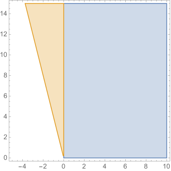
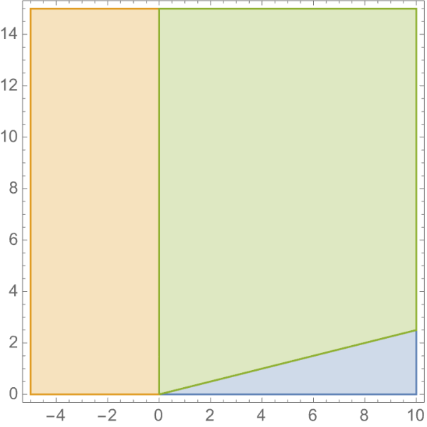
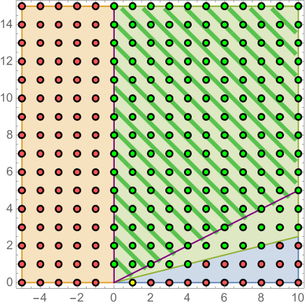
As an example for the single flop case, we discuss the $h^{1,1}(X)=2$ complete intersection Calabi-Yau manifolds $X$ given as hypersurfaces of degree $(2,4)$ in the ambient space $\mathbbm{P}^{1}\times\mathbbm{P}^{3}$ (CICY 7887 in the list of Ref. [12]). Choosing the divisors $(D_{1},D_{2})$ as the Poincare duals of the standard Kähler forms of the ambient projective factors restricted to $X$, the Kähler cone relative to this basis is indeed given by the positive quadrant, $\mathcal{K}=\{t_{1}e_{1}+t_{2}e_{2}\,|\,t^{i}\geq 0\}$. The non-zero intersection numbers $\lambda_{ijk}=D_{i}\cdot D_{j}\cdot D_{k}$ are $\lambda_{122}=4$ and $\lambda_{222}=2$. Inserting these numbers into Eqs. (2.1) gives $m_{1}=4$ while $m_{2}\not\in\mathbbm{Z}$, which indicates we have indeed a flop boundary at $\{t^{1}=0\}$ while $\{t^{2}=0\}$ is a boundary of the effective cone. As a consequence, we have

The resulting Kähler cone structure

where $\tilde{v}_{1}=(-1,4)^{T}$, is shown in Figure 1 on the left. For the dual cones this means

where $v_{1}=(4,1)^{T}$ and $w=(2,1)^{T}$. The dual cones and the restricted cones are illustrated in Figure 1 in the middle. The structure of GV invariants is indicated in Figure 1 on the right. Flopping classes correspond to yellow dots, so for this example there is only a single flopping class, $\mathcal{B}=\{(1,0)\}$, with GV invariant $n_{(1,0)}=64$. Red points indicate classes with vanishing GV invariants while the GV invariants for the green points, contained in the restricted cone, can be positive. The green, hatched region is the fundamental region $\mathcal{K}_{f}$. Inserting this into Eq. (2.10) with $\Psi_{d}^{G}$ defined in Eq. (2.11), we get the instanton prepotential

where the summation range $\mathcal{K}_{f}$ is as in Eq. (2.2).

Out of the $36$ manifolds with $h^{1,1}(X)=2$, defined as complete intersections in product of projective spaces, there are 20, including the above example, with a single flop, as can be seen from the Appendix A of [5]. There are also $36$ Kreuzer-Skarke CY manifolds with $h^{1,1}(X)=2$ and Appendix B of [5] shows at least $16$ of those are single-flop cases. All of these manifolds have a prepotential with a structure similar to Eq. (2.17).

To uncover the structure of $G$, it is convenient to introduce the matrices

Then, every group element can be written in the form $Q^{k}S^{\alpha}$, where $\alpha\in\{0,1\}$ and $k\in\mathbb{Z}$. Clearly, $S$ has order two and generates a sub-group of $G$ isomorphic to $\mathbb{Z}_{2}$. On the other hand, the order $N$ of $Q$ can be finite or infinite, depending on the value of $m_{1}m_{2}$, and the group $\mathbb{Z}_{N}$ (with $\mathbb{Z}_{\infty}=\mathbb{Z}$) it generates is normal in $G$. So in conclusion, we have $G\cong\mathbb{Z}_{N}\rtimes\mathbb{Z}_{2}$. It remains to determine the order $N$ and the precise form of the matrices $Q^{k}S^{\alpha}$ and to do this we need to distinguish the three cases mentioned above.

For the remainder of this section, we will focus on the case $m_{1}m_{2}>4$, the only one actually realized for $h^{1,1}(X)=2$. The group $G$ consists of elements $Q^{k}S^{\alpha}$, where $k\in\mathbb{Z}$ and $\alpha\in\{0,1\}$, with the matrices $S$ and $Q$ from Eq. (3.9) and it is isomorphic to $\mathbbm{Z}\rtimes\mathbbm{Z}_{2}$. In addition to the “central” Kähler cone $\mathcal{K}$ of $X$ we have an infinite number of isomorphic CYs with adjacent Kähler cones $\mathcal{K}_{\tilde{g}}=\tilde{g}\mathcal{K}$ to either side of $\mathcal{K}$. The union of these forms the effective cone

where

Note that for the case $m_{1}m_{2}>4$ the closure of this cone is irrational. For a specific example, the extended cone is shown in Fig. 2 on the left. The Mori cones dual of the Kähler cones $\mathcal{K}_{\tilde{g}}$ are denoted by $\mathcal{M}_{g}=g\mathcal{M}$ and their intersection, which is the dual of the effective cone, forms the restricted cone

An example of a restricted cone is shown in Figure 2, in the middle.

In our discussion of the GV invariants we will distinguish again between flopping and non-flopping classes. The flopping classes $\mathcal{B}$ of the original manifold $X$ are contained in $\mathcal{B}\subset\{(1,0),(2,0),(0,1),(0,2)\}$, straightforwardly generalizing what we have seen in the single-flop case. As before, for a flopping class $d\in\mathcal{B}$ of $X$, its images $gd$ under the group $G$ are also flopping classes, but rather for one of the isomorphic manifolds $X^{\prime}$ instead of $X$. Hence, for every flopping class $d\in\mathcal{B}$ of $X$ we have an entire infinite $G$-orbit of flopping classes (while, for the single flop case where $G\cong\mathbb{Z}_{2}$ the orbits only had length two). We have already seen that GV invariants are not constant along these orbits. Rather, for a flopping class $d\in\mathbb{B}$ of $X$ we have

As before, non-flopping classes $d$ outside the restricted cone always have vanishing GV invariants, $n_{d}=0$. The restricted cone is $G$-invariant and it splits into $G$-orbits on which the GV invariants are constant, so $n_{gd}=n_{d}$ for $d\in\mathcal{M}_{\rm restr}$ and all $g\in G$. Within the restricted cone we can choose a fundamental region for the $G$-action as

For our example, the structure of the various cones and the GV invariants is indicated in Figure 2, on the right.

Now we have everything in place to write down an expression for the instanton prepotential. As before, we split the sum into flopping and non-flopping classes, using (3.2) for the former and $G$-invariance of the GV invariants for the latter. This leads to

with the $G$-invariant functions

The functions (3.38) contain the matrix powers $Q^{k}$ from (3.1) in their exponents and, hence, these exponents increase with powers of $k$. Functions that behave in this way are not modular – the exponents for modular functions depend quadratically on $k$. To the best of our knowledge, the functions $\Psi_{d}^{G}$ in Eq. (3.38) have not been studied before and they do not have an established name. It would be interesting to analyze their properties in more detail.

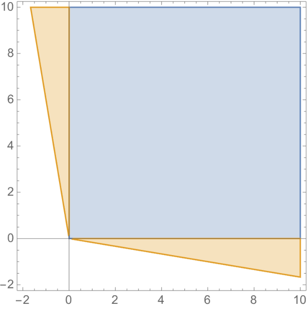
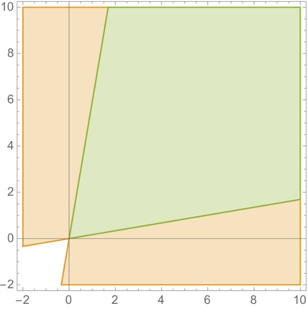
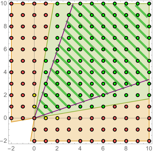
We would like to illustrate the above structure with a specific example, the complete intersection CY manifold described by the configuration matrix

This is CICY 7863 in the standard list of Ref. [12] and it has Hodge numbers $(h^{1,1},h^{2,1})=(2,68)$. The above configuration matrix indicates that the manifold $X$ is defined as the common zero locus of three polynomials in $\mathbb{P}^{3}\times\mathbb{P}^{3}$ with bi-degrees $(2,2)$, $(1,1)$ and $(1,1)$. The Kähler cone $\mathcal{K}$ (relative to the standard divisor basis $(D_{1},D_{2})$ associated to pullbacks of the hyperplane classes of the ambient space $\mathbb{P}^{3}$ factors) is the positive quadrant and the non-zero intersection numbers are given by $\lambda_{111}=\lambda_{222}=2$ and $\lambda_{112}=\lambda_{122}=6$. Equation (2.1) implies that $m_{1}=m_{2}=6$ and hence both boundaries, $\{t^{1}=0\}$ and $\{t^{2}=0\}$, exhibit isomorphic flops, resulting in an infinite flop sequence. The various cones are shown in Figure 2.

The flopping classes of $X$ are given by $\mathcal{B}=\{(1,0),(2,0),(0,1),(0,2)\}$ (indicated by yellow dots in Figure 2 on the right) with $n_{(1,0)}=n_{(0,1)}=80$ and $n_{(2,0)}=n_{(0,2)}=4$. Hence, the first sum in (3.37) runs over four (partial) $G$-orbits. For the elements of $G$ we have

where we have defined

Inserting this into (3.38), we get the the $G$-invariant functions $\Psi_{d}^{G}$

As can be seen from Appendix A of Ref. [5], among the $h^{1,1}(X)=2$ CICYs, there are six manifolds with infinite flop sequences (including the above example) which realize the values

They can be analyzed along the same lines as the example above.

We can assume that the two flop boundaries are $\{t^{1}=0\}$ and $\{t^{2}=0\}$, so that the corresponding generators can be written as

These $(h\times h)$ matrices $\mathcal{M}_{i}$ are block matrices consisting of a $2\times 2$ block $M_{i}$ from Eq. (3), a $2\times(h-2)$ block $U_{i}$, an $(h-2)\times 2$ block with the zero-matrix, and a $(h-2)\times(h-2)$ identity matrix. The $1\times(h-2)$-dimensional row vectors $u_{1}$ and $u_{2}$ are defined in terms of the GLSM charges as explained in Ref. [4] and reviewed in Appendix A. If we define new generators

the elements of $G=\langle\mathcal{M}_{1},\;\mathcal{M}_{2}\rangle$ can be uniquely written as $\mathcal{Q}^{k}\mathcal{S}^{\alpha}$, where $k\in\mathbbm{Z}$ and $\alpha\in\{0,1\}$. More explicitly, these matrices are

References

- [1] P. S. Aspinwall, B. R. Greene, and D. R. Morrison “Multiple mirror manifolds and topology change in string theory,” Phys. Lett. B 303 (1993) 249–259 [hep-th/9301043].
- [2] P. S. Aspinwall, B. R. Greene, and D. R. Morrison “Calabi-Yau moduli space, mirror manifolds and space-time topology change in string theory,” Nucl. Phys. B 416 (1994) 414–480 [hep-th/9309097].
- [3] B. R. Greene “String theory on Calabi-Yau manifolds,” in Theoretical Advanced Study Institute in Elementary Particle Physics (TASI 96): Fields, Strings, and Duality pp. 543–726. 6, 1996. [hep-th/9702155].
- [4] C. Brodie, A. Constantin, A. Lukas, and F. Ruehle “Flops for Complete Intersection Calabi-Yau Threefolds,” [2112.12106].
- [5] C. R. Brodie, A. Constantin, A. Lukas, and F. Ruehle “Geodesics in the extended Kähler cone of Calabi-Yau threefolds,” JHEP 03 (2022) 024 [2108.10323].
- [6] C. R. Brodie, A. Constantin, and A. Lukas “Flops, Gromov-Witten invariants and symmetries of line bundle cohomology on Calabi-Yau three-folds,” J. Geom. Phys. 171 (2022) 104398 [2010.06597].
- [7] H. S. M. Coxeter “Discrete groups generated by reflections,” Annals of Mathematics 35 588–621.
- [8] È. B. Vinberg “DISCRETE LINEAR GROUPS GENERATED BY REFLECTIONS,” Mathematics of the USSR-Izvestiya 5 (oct, 1971) 1083–1119.
- [9] N. Gendler, M. Kim, L. McAllister, J. Moritz, and M. Stillman “Superpotentials from Singular Divisors,” [2204.06566].
- [10] R. Gopakumar and C. Vafa “M theory and topological strings. 1.,” [hep-th/9809187].
- [11] R. Gopakumar and C. Vafa “M theory and topological strings. 2.,” [hep-th/9812127].
- [12] P. Candelas, A. M. Dale, C. A. Lutken, and R. Schimmrigk “Complete Intersection Calabi-Yau Manifolds,” Nucl. Phys. B298 (1988) 493.
- [13] P. Candelas, X. de la Ossa, P. Kuusela, and J. McGovern “Mirror Symmetry for Five-Parameter Hulek-Verrill Manifolds,” [2111.02440].
- [14] K. Hulek and H. Verrill “On modularity of rigid and nonrigid calabi-yau varieties associated to the root lattice a 4,” Nagoya Mathematical Journal 179 (2005) 103–146.
- [15] P. Candelas, X. C. De La Ossa, P. S. Green, and L. Parkes “A Pair of Calabi-Yau manifolds as an exactly soluble superconformal theory,” Nucl. Phys. B 359 (1991) 21–74.
- [16] M. C. N. Cheng, J. F. R. Duncan, and J. A. Harvey “Weight One Jacobi Forms and Umbral Moonshine,” J. Phys. A 51 (2018) no. 10, 104002 [1703.03968].
- [17] M.-x. Huang, S. Katz, and A. Klemm “Topological String on elliptic CY 3-folds and the ring of Jacobi forms,” JHEP 10 (2015) 125 [1501.04891].
- [18] P. Candelas, X. de la Ossa, M. Elmi, and D. Van Straten “A One Parameter Family of Calabi-Yau Manifolds with Attractor Points of Rank Two,” JHEP 10 (2020) 202 [1912.06146].
- [19] K. Bönisch, F. Fischbach, A. Klemm, C. Nega, and R. Safari “Analytic structure of all loop banana integrals,” JHEP 05 (2021) 066 [2008.10574].
- [20] C. R. Brodie, A. Constantin, A. Lukas, and F. Ruehle “Swampland conjectures and infinite flop chains,” Phys. Rev. D 104 (2021) no. 4, 046008 [2104.03325].
- [21] J. Gray, A. S. Haupt, and A. Lukas “Topological Invariants and Fibration Structure of Complete Intersection Calabi-Yau Four-Folds,” JHEP 09 (2014) 093 [1405.2073].