跳到论文正文
W Papers独立论文阅读器 arXiv:2210.09354 论文正文 计算阅读时间 · 0%
引用这篇论文根据当前论文元数据生成,正式投稿前建议核对。


License: arXiv.org perpetual non-exclusive license
arXiv:2210.09354v2 [math.AP] 05 Nov 2022

Decomposition of the Wave Manifold into Lax Admissible Regions and its Application to the Solution of Riemann Problems

Cesar S. Eschenazi Thanks: email: cseschenazi@gmail.com Affiliation: Universidade Federal de Minas Gerais – UFMG
Belo Horizonte, MG, CEP: 31270-901
   Wanderson J. Lambert Thanks: email: wanderson.lambert@unifal-mg.edu.br Affiliation: Universidade Federal de Alfenas – UNIFAL
Alfenas, MG, CEP: 37130-001
   Marlon M. López-Flores Thanks: email: mmlf@impa.br Affiliation: Instituto Nacional de Matemática Pura e Aplicada – IMPA
Rio de Janeiro, RJ, Brazil, CEP: 22460-320
   Dan Marchesin Thanks: email: marchesi@impa.br Affiliation: Instituto Nacional de Matemática Pura e Aplicada – IMPA
Rio de Janeiro, RJ, Brazil, CEP: 22460-320
   Carlos F.B. Palmeira Thanks: email: fredpalm@gmail.com - Corresponding author. Affiliation: Pontifícia Universidade Católica do Rio de Janeiro – PUC-Rio
Rio de Janeiro, RJ - Brasil, CEP: 22451-900
Abstract

We utilize a three-dimensional manifold to solve Riemann Problems that arise from a system of two conservation laws with quadratic flux functions. Points in this manifold represent potential shock waves, hence its name wave manifold. This manifold is subdivided into regions according to the Lax admissibility inequalities for shocks. Finally, we present solutions for the Riemann Problems for various cases and exhibit continuity relative to LL and RR data, despite the fact that the system is not strictly hyperbolic. The usage of this manifold regularizes the solutions despite the presence of an elliptic region.

1 Introduction

We consider the system of two partial differential equations

Wt+F(W)x=0,\left.W_{{}_{t}}+F(W)_{{}_{x}}=0,\right. (1.1)

with initial conditions

W⁡(x,t=0)={WLif ​x<0,WRif ​x>0.W(x,t=0)=\left\{\begin{array}[]{ll}W_{{}_{L}}&\hbox{\rm{if }}x<0,\\ W_{{}_{R}}&\hbox{\rm{if }}x>0.\end{array}\right. (1.2)

We will take W=(u,v)∈ℝ2W=(u,v)\in\mathbb{R}^{{}^{2}} and FF a map F:ℝ2⟶ℝ2F:\mathbb{R}^{{}^{2}}\longrightarrow\mathbb{R}^{{}^{2}}, the two components of which are called flux functions. Equation (1.1) appears in fluid dynamics and together with initial conditions (1.2) is called a Riemann problem.

We are mainly interested in the so called shock solutions, defined by

W={Wfor ​x<s​t,W′for ​x>s​t,W=\left\{\begin{array}[]{ll}W&\hbox{\rm{for }}x<st,\\ W^{\prime}&\hbox{\rm{for }}x>st,\end{array}\right.

where ss is the shock propagation speed, W=(u,v)W=(u,v) and W′=(u′,v′)W^{\prime}=(u^{\prime},v^{\prime}) are the states to be connected by the shock.

In order to have physical meaning as a shock, the speed and the states must satisfy the so called Rankine-Hugoniot condition [10].

F⁡(W)−F⁡(W′)=s⁡(W−W′),F(W)-F(W^{\prime})=s(W-W^{\prime}), (1.3)

for some ss. This leads to the definition of Hugoniot curve associated to a given state W=(u0,v0)W=(u_{{}_{0}},v_{{}_{0}}), in Section 2.

Furthermore, not all arcs of Hugoniot curves are useful to construct solutions. Shock curve arcs must satisfy some extra conditions called admissibility conditions. In [1], Liu’s admissibility entropy criterion was introduced within the wave manifold context. There it was shown that under certain extra assumptions, which will be considered in the current paper, Liu’s entropy criterion can be replaced by the Lax entropy inequality conditions. These inequalities relate ss and the eigenvalues of D​F​(u,v)DF(u,v). Hugoniot arc curves satisfying these inequalities are called shock curve arcs or admissible arcs.

We adopt here the topological point of view, as described in [5]. We consider the space ℝ5\mathbb{R}^{{}^{5}} of coordinates (u,v,u′,v′,s)(u,v,u^{\prime},v^{\prime},s) and in it the three-dimensional manifold defined by F⁡(u,v)−F⁡(u′,v′)−s⁡(u−u′,v−v′)=0F(u,v)-F(u^{\prime},v^{\prime})-s(u-u^{\prime},v-v^{\prime})=0. In this manifold, we consider the curves defined by (u,v)(u,v) constant, called Hugoniot curves, their projections onto the state space are the classical Rankine-Hugoniot curves, see [1]. This manifold is called wave manifold.

In a series of papers (see [1, 3, 7, 8]), this manifold and its Hugoniot curves have been studied for the case where FF is a polynomial of degree two. The wave manifold has been characterized, relevant surfaces (c​h​a​r​a​c​t​e​r​i​s​t​i​ccharacteristic, s​o​n​i​csonic and s​o​n​i​c′sonic^{\prime}) have been defined, the intersection of Hugoniot curves with these surfaces has been studied, and the Lax inequalities have been interpreted in this context. Here, also considering FF as a polynomial of degree two, we decompose the c​h​a​r​a​c​t​e​r​i​s​t​i​ccharacteristic and s​o​n​i​c′sonic^{\prime} surfaces in their fast and slow components. And also decompose the wave manifold in regions which we call admissible or non-admissible regions.

As stated at the beginning of Section 2, we will restrict ourselves to the symmetric Case IV of the Sheaffer-Shearer classification, see [9]. A study of cases I, II, III and IV (non symmetric case) can be found in [6].

We will also consider rarefaction and composite solutions, to be defined in Section 7 and used in Sections 8 and 9.

This paper is organized as follows: In Section 2, we review some basic facts and definitions, introduce new variables and describe the c​h​a​r​a​c​t​e​r​i​s​t​i​ccharacteristic, s​o​n​i​csonic and s​o​n​i​c′sonic^{\prime} surfaces, [5]. In Section 3, we characterize the slow and fast components of the characteristic surface associated with the eigenvalues of D​FDF. We also characterize the coincidence curve, which is the boundary of these two components. In Section 4, we describe how the c​h​a​r​a​c​t​e​r​i​s​t​i​ccharacteristic, s​o​n​i​csonic and s​o​n​i​c′sonic^{\prime} surfaces divide the wave manifold into twelve regions and characterize the surface formed by the Hugoniot curves through points of the coincidence curve. This surface will be called saturated of the coincidence curve by Hugoniot curves and denoted by S​S​CSSC. It is tangent to the c​h​a​r​a​c​t​e​r​i​s​t​i​ccharacteristic and s​o​n​i​c′sonic^{\prime} surfaces. In Section 5, we characterize the slow and fast components of the s​o​n​i​c′sonic^{\prime} surface, associated with the slow shock speed and the fast shock speed. We show that the boundaries of these two components are a straight line and the hysteresis′ curve, which is the curve where Hugoniot curves are tangent to the s​o​n​i​c′sonic^{\prime} surface. In Section 6, we identify some of regions in the wave manifold where Lax’s inequalities are satisfied, indicating in which regions there are local shock curve arcs and in which of these regions there are nonlocal shock curve arcs.

In Section 7, we present the rarefaction and composite curves, derived from the rarefaction solutions mentioned before, and decompose the state space ((u,v)(u,v)-plane) in elliptic and hyperbolic regions. In Section 8, we introduce the wave curve in the wave manifold, such curves consist of arcs of admissible Hugoniot curves, rarefaction curves and composite curves of the same family. In Section 9, we use all the elements previously defined to solve Riemann problems.

It is known from [3] that a Hugoniot curve through points of the secondary bifurcation has two components, a straight line and a curve. The lines generate a plane and the curves a surface, which we will call saturated of secondary bifurcation by Hugoniot curves, denoted by S​S​BSSB. In Appendix 1, we characterize the regions of the wave manifold where condition L2, introduced in Section 6, is satisfied. In Appendix 3, we justify the choices of the flux function, parameters and coordinates used in this paper.

2 The Wave Manifold and Hugoniot Curves

In this section, we review some basic facts and definitions and introduce new variables. We will define the c​h​a​r​a​c​t​e​r​i​s​t​i​ccharacteristic, s​o​n​i​csonic and s​o​n​i​c′sonic^{\prime} surfaces, since they will appear as boundaries of the admissible regions.

We refer the reader to Section 2 of [3] for basic definitions. For the sake of completeness, we briefly present some necessary concepts needed here.

We consider the equation (1.1) with FF given by F=(f,g)F=(f,g), where

{f(u,v)=v2/2+(b1+1)u2/2+a1u+a2v,g(u,v)=uv+a3u+a4v,\left\{\begin{array}[]{l}f(u,v)=v^{{}^{2}}/2+(b_{{}_{1}}+1)u^{{}^{2}}/2+a_{{}_{1}}u+a_{{}_{2}}v,\\ \\ g(u,v)=uv+a_{{}_{3}}u+a_{{}_{4}}v,\end{array}\right. (2.1)

for b1>1b_{{}_{1}}>1. This is the symmetric Case IV in the Schaeffer and Shearer classification, see [9].

Given a point W=(u,v)W=(u,v), in the (usually called) “state space”, the Hugoniot curve through this point is defined as the set of points W′=(u′,v′)W^{\prime}=(u^{\prime},v^{\prime}), such that there exists ss such that satisfies F⁡(W)−F⁡(W′)=s⁡(W−W′)F(W)-F(W^{\prime})=s(W-W^{\prime}). We clearly see that this curve passes through WW.

To study Hugoniot curves, we consider ℝ5={(u,v,u′,v′,s)}\mathbb{R}^{{}^{5}}=\{(u,v,u^{\prime},v^{\prime},s)\} and in it the three-dimensional manifold defined by F⁡(W)−F⁡(W′)=s⁡(W−W′)F(W)-F(W^{\prime})=s(W-W^{\prime}). Since this manifold is singular along the diagonal W=W′W=W^{\prime}, along this diagonal, we perform a blow up, which, in this simple case, is obtained using the coordinate transformations given by U=(u+u′)/2U=(u+u^{\prime})/2, V=(v+v′)/2V=(v+v^{\prime})/2, X=u−u′X=u-u^{\prime}, Y=v−v′Y=v-v^{\prime}, and Z=Y/XZ=Y/X and factoring X2X^{{}^{2}}. We also set c=a3−a2>0c=a_{{}_{3}}-a_{{}_{2}}>0. Using these new coordinates, we get

(1−Z2)(V+a2)−Z(b1U+a1−a4)+c=0andY=ZX.(1-Z^{{}^{2}})\left(V+a_{{}_{2}}\right)-Z\left(b_{{}_{1}}U+a_{{}_{1}}-a_{{}_{4}}\right)+c=0\ \ \ \ \ \ \ \text{and}\ \ \ \ \ \ \ Y=ZX.

The two above equations define a regular three-dimensional manifold, which will be referred as the wave manifold and will be denoted by 𝒲\mathcal{W}.

Since ZZ is a direction, we may think of the wave manifold 𝒲\mathcal{W}, as contained in ℝ4×ℝP1\mathbb{R}^{{}^{4}}\times\mathbb{R}P^{{}^{1}}, or, which is the same as, ℝ4×S1\mathbb{R}^{{}^{4}}\times S^{{}^{1}}. These coordinates are not valid at Z=∞Z=\infty, but there are no special features at infinity, so, we can just use XX, UU, VV, ZZ to study Hugoniot curves.

Defining U~=b1U+a1−a4\widetilde{U}=b_{{}_{1}}U+a_{{}_{1}}-a_{{}_{4}} and V~=V+a2\widetilde{V}=V+a_{{}_{2}} we obtain the equation G1=(1−Z2)V~−ZU~+c=0G_{{}_{1}}=(1-Z^{{}^{2}})\widetilde{V}-Z\widetilde{U}+c=0, used in ([7, 3, 4]).

Hugoniot curves in the wave manifold are defined by u=constantu=\text{constant} and v=constantv=\text{constant}, which, in these new coordinates, become

{2U~+b1X=2b1u0+2(a1−a4),2V~+ZX=2v0+2a2.\left\{\begin{array}[]{l}2\widetilde{U}+b_{{}_{1}}X=2b_{{}_{1}}u_{{}_{0}}+2(a_{{}_{1}}-a_{{}_{4}}),\\ 2\widetilde{V}+ZX=2v_{{}_{0}}+2a_{{}_{2}}.\end{array}\right. (2.2)

As shown in [7], Hugoniot curves are connected and foliate 𝒲\mathcal{W} except along a straight line BB, contained on the plane, Π\Pi, defined by Z=0Z=0. The straight line BB is called secondary bifurcation. Hugoniot curves through points in BB are formed by two arcs: a straight line h​u​g​lhugl and a curve h​u​g​chugc. These two arcs intersect at a point of BB. The lines h​u​g​lhugl fill the plane Π\Pi.

Definition 1.

The set of Hugoniot curves through points of h​u​g​chugc is called saturated of the secondary bifurcation by Hugoniot curves and denoted by S​S​BSSB.

It is easy to see that S​S​BSSB is a two-dimensional sub-manifold of 𝒲\mathcal{W} and that S​S​BSSB and Π\Pi intersect transversely along BB.

The same conclusions are valid for Hugoniot′ curves, defined by u′=c​o​n​s​t​a​n​tu^{\prime}=constant and v′=c​o​n​s​t​a​n​tv^{\prime}=constant. Hugoniot′ curves are connected and foliate 𝒲\mathcal{W} except along a straight line B′B^{\prime}, also contained on the plane Π\Pi. Hugoniot′ curves through points in B′B^{\prime} are formed by two arcs: a straight line h​u​g​l′hugl^{\prime} and a curve h​u​g​c′hugc^{\prime}. These two arcs intersect at a point of B′B^{\prime}. The lines h​u​g​l′hugl^{\prime} also fill the plane Π\Pi. In a similar way the curves h​u​g​c′hugc^{\prime} form a two-dimensional sub-manifold called saturated of the secondary bifurcation by Hugoniot′ curves, denoted by S​S​B′SSB^{\prime}. The plane Π\Pi and intersect transversely along B′B^{\prime}.

There are three important surfaces in the study of the wave manifold: Characteristic (denoted by 𝒞\mathcal{C}), Sonic (denoted by S​o​nSon) and Sonic′ (denoted by S​o​n′Son^{\prime}).

To define S​o​nSon and S​o​n′Son^{\prime}, one must look at the speed ss as a real function in 𝒲\mathcal{W} given by[f⁡(u,v)−f⁡(u′,v′)]/(u−u′)[f(u,v)-f(u^{\prime},v^{\prime})]/(u-u^{\prime}) or [g⁡(u,v)−g⁡(u′,v′)]/(v−v′)[g(u,v)-g(u^{\prime},v^{\prime})]/(v-v^{\prime}). Using coordinates XX, U~\widetilde{U} and V~\widetilde{V}, we have

s=U~b1+V~Z,\left.s=\frac{\widetilde{U}}{b_{{}_{1}}}+\frac{\widetilde{V}}{Z},\right. (2.3)

To define S​o​nSon, we restrict ss to a Hugoniot curve, and look at its critical points. The set of these critical points for all Hugoniot curves is the Sonic surface, S​o​nSon. In the same way, we define the S​o​n​i​c′Sonic^{\prime} surface, S​o​n′Son^{\prime}, as the set of all critical points of ss restricted to a Hugoniot′ curve. This was done in [7], obtaining equations

2[Z2+b1+1]U~+2[Z3+(b1+3)Z]V~−[Z2−(b1+1)]X=02[Z^{{}^{2}}+b_{{}_{1}}+1]\widetilde{U}+2[Z^{{}^{3}}+(b_{{}_{1}}+3)Z]\widetilde{V}-[Z^{{}^{2}}-(b_{{}_{1}}+1)]X=0 (2.4)

for S​o​nSon and

2[Z2+b1+1]U~+2[Z3+(b1+3)Z]V~+[Z2−(b1+1)]X=02[Z^{{}^{2}}+b_{{}_{1}}+1]\widetilde{U}+2[Z^{{}^{3}}+(b_{{}_{1}}+3)Z]\widetilde{V}+[Z^{{}^{2}}-(b_{{}_{1}}+1)]X=0 (2.5)

for S​o​n′Son^{\prime}.

We list some important known facts about 𝒞\mathcal{C}, S​o​nSon and S​o​n′Son^{\prime}, for the quadratic flux functions considered here.

Fact 1.- 𝒞\mathcal{C} is topologically a cylinder.

Fact 2.- Given a Hugoniot curve, either it intersects 𝒞\mathcal{C} transversely in two points, or it is tangent or it does not intersect 𝒞\mathcal{C}.

Fact 3.- The above mentioned set of tangency points form a simple closed curve. This curve does not bound a disk in 𝒞\mathcal{C} and divides it into two components, denoted by 𝒞s\mathcal{C}_{{}_{s}} and 𝒞f\mathcal{C}_{{}_{f}}. This simple closed curve is called coincidence curve in 𝒞\mathcal{C}, denoted by ℰ𝒞\mathcal{E_{C}}.

Fact 4.- Any Hugoniot curve through a point 𝒰\mathcal{U}, s​h​(𝒰)sh(\mathcal{U}), which intersects 𝒞\mathcal{C} transversely, does it at a point 𝒰s=sh(𝒰)∩𝒞s\mathcal{U}_{{}_{s}}=sh(\mathcal{U})\cap\mathcal{C}_{{}_{s}} and in another point 𝒰f=sh(𝒰)∩𝒞f\mathcal{U}_{{}_{f}}=sh(\mathcal{U})\cap\mathcal{C}_{{}_{f}}. The value of the speed ss in 𝒰s\mathcal{U}_{{}_{s}} is smaller than the value of ss in 𝒰f\mathcal{U}_{{}_{f}}. Proof of this fact will be presented in Section 3, where we will characterize 𝒞s\mathcal{C}_{{}_{s}} and 𝒞f\mathcal{C}_{{}_{f}}.

Fact 5.- S​o​nSon and S​o​n′Son^{\prime} are topologically Möbius band and they intersect 𝒞\mathcal{C} along a curve called inflection locus, denoted by ℐ\mathcal{I}, which is diffeomorphic to ℝ\mathbb{R}, and contains the intersection point of BB and 𝒞\mathcal{C}. They also intersect along two straight lines, each of which intersects transversally 𝒞\mathcal{C} at a point of the inflection locus.

Fact 6.- Generically, a Hugoniot curve through a point 𝒰\mathcal{U}, s​h​(𝒰)sh(\mathcal{U}), intersects S​o​n′Son^{\prime} in 0, 2 or 4 points. If s​h​(𝒰)∩S​o​n′sh(\mathcal{U})\cap Son^{\prime} has 2 points, then ss has the same value in these 2 points as the value of ss either in 𝒰s\mathcal{U}_{{}_{s}} or in 𝒰f\mathcal{U}_{{}_{f}}. In the first case, the points are said to be in S​o​ns′Son^{\prime}_{s} and in the second case, in Son′fSon^{\prime}_{{}_{f}}. If the intersection has 4 points, then ss has the same value of ss in 𝒰s\mathcal{U}_{{}_{s}} in two of them and the value of ss in 𝒰f\mathcal{U}_{{}_{f}} in the other two. The first two are points in S​o​ns′Son^{\prime}_{s} and the other two in Son′fSon^{\prime}_{{}_{f}}.

2.1 New Coordinates

In this paper, we use coordinates z=1/Zz=1/Z, tt and YY. The main advantage is that they are valid for 𝒲−Π\mathcal{W}-\Pi and Π\Pi becomes the plane z=∞z=\infty. To define tt, we start by writing the equation of 𝒲\mathcal{W} in term of the variables U~\widetilde{U}, V1=V+a3=V~+cV_{{}_{1}}=V+a_{{}_{3}}=\widetilde{V}+c and zz. We get G=0G=0, where G=(z2−1)V1−zU~+cG=(z^{{}^{2}}-1)V_{{}_{1}}-z\widetilde{U}+c. The parameter tt is defined by

U~=2​c​zz2+1+ct(z2−1)andV1=cz2+1+ctz.\widetilde{U}=\displaystyle\frac{2cz}{z^{{}^{2}}+1}+ct(z^{{}^{2}}-1)\ \ \ \ \ \ \ \text{and}\ \ \ \ \ \ \ V_{{}_{1}}=\displaystyle\frac{c}{z^{{}^{2}}+1}+ctz. (2.6)

For each fixed zz, the parameter tt measures as far as U~\widetilde{U} and V1V_{{}_{1}} are away from the coincidence curve in 𝒞\mathcal{C} in the orthogonal direction to it.

In these new coordinates, the characteristic surface, 𝒞\mathcal{C}, is the plane Y=0Y=0. The sonic and the s​o​n​i​c′sonic^{\prime} surfaces are given by the equations obtained from equations (2.4) and (2.5) by transforming from variables U~\widetilde{U}, V~\widetilde{V}, XX and ZZ to the new coordinates zz, tt and YY. We obtain s​o​n=0son=0, where

son=−2c[(b1+1)z5+(b1+4)z3+3z]t−[(b1+1)z4+b1z2−1]Y−2c[(b1−1)z2+1],son=-2c[(b_{{}_{1}}+1)z^{{}^{5}}+(b_{{}_{1}}+4)z^{{}^{3}}+3z]t-[(b_{{}_{1}}+1)z^{{}^{4}}+b_{{}_{1}}z^{{}^{2}}-1]Y-2c[(b_{{}_{1}}-1)z^{{}^{2}}+1], (2.7)

and s​o​n′=0son^{\prime}=0, where

son′=−2c[(b1+1)z5+(b1+4)z3+3z]t+[(b1+1)z4+b1z2−1]Y−2c[(b1−1)z2+1].son^{\prime}=-2c[(b_{{}_{1}}+1)z^{{}^{5}}+(b_{{}_{1}}+4)z^{{}^{3}}+3z]t+[(b_{{}_{1}}+1)z^{{}^{4}}+b_{{}_{1}}z^{{}^{2}}-1]Y-2c[(b_{{}_{1}}-1)z^{{}^{2}}+1]. (2.8)

The shock speed, ss, is written as

s=c[(b1+1)tz4+b1z2t+(b1+2)z−t]b1(z2+1).s=\displaystyle\frac{c[(b_{{}_{1}}+1)tz^{{}^{4}}+b_{{}_{1}}z^{{}^{2}}t+(b_{{}_{1}}+2)z-t]}{b_{{}_{1}}(z^{{}^{2}}+1)}. (2.9)

Parametric equations for Hugoniot curves in zz, tt, YY coordinates are obtained by replacing U~\widetilde{U}, V~\widetilde{V} and XX into equations in (2.2), by their values in terms of zz, tt, YY and solving the system with respect to tt and YY. We get:

{z=z,t=(v0+a3)b1z3+(b1u0+a1−a4)z2−[b1(v0+a2)+2c]z+b1u0+a1−a4c(z2+1)[(b1−1)z2+1],Y=−2(v0+a3)z2+2(b1u0+a1−a4)z+2(v0+a2)(b1−1)z2+1.\left\{\begin{array}[]{l}z=z,\\ t=\displaystyle\frac{(v_{{}_{0}}+a_{{}_{3}})b_{{}_{1}}z^{{}^{3}}+(b_{{}_{1}}u_{{}_{0}}+a_{{}_{1}}-a_{{}_{4}})z^{{}^{2}}-[b_{{}_{1}}(v_{{}_{0}}+a_{{}_{2}})+2c]z+b_{{}_{1}}u_{{}_{0}}+a_{{}_{1}}-a_{{}_{4}}}{c(z^{{}^{2}}+1)[(b_{{}_{1}}-1)z^{{}^{2}}+1]},\\ Y=\dfrac{-2(v_{{}_{0}}+a_{{}_{3}})z^{{}^{2}}+2(b_{{}_{1}}u_{{}_{0}}+a_{{}_{1}}-a_{{}_{4}})z+2(v_{{}_{0}}+a_{{}_{2}})}{(b_{{}_{1}}-1)z^{{}^{2}}+1}.\end{array}\right. (2.10)

From the expression of YY in (2.10), we see that a Hugoniot curve intersects 𝒞\mathcal{C} depending on whether ℰs​s=(b1u0+a1−a4)2+4(v0+a3)(v0+a2)\mathcal{E}_{{}_{ss}}=(b_{{}_{1}}u_{{}_{0}}+a_{{}_{1}}-a_{{}_{4}})^{{}^{2}}+4(v_{{}_{0}}+a_{{}_{3}})(v_{{}_{0}}+a_{{}_{2}}) is positive or negative: It intersects 𝒞\mathcal{C} in two points if ℰs​s>0\mathcal{E}_{{}_{ss}}>0 and does not intersect 𝒞\mathcal{C} if ℰs​s<0\mathcal{E}_{{}_{ss}}<0.

Definition 2.

The curve ℰs​s=0\mathcal{E}_{{}_{ss}}=0 is called coincidence curve in the state space, it is an ellipse. Its interior is called elliptic region and its exterior is called hyperbolic region.

As we shall see in Subsection 7.1, there are no rarefaction curves through points of the elliptic region and through every point of the hyperbolic region pass two transversal rarefaction curves.

Parametric equations for Hugoniot′ curves are obtained from equations (2.10) by interchanging YY with −Y-Y.

Substituting the second equation of (2.10) into equation (2.9), we get the expression of the shock speed s=s(u0,v0,z)s=s(u_{{}_{0}},v_{{}_{0}},z) along a Hugoniot curve.

In order to get the expression of a Hugoniot curve through a given point (z0,t0,Y0)(z_{{}_{0}},t_{{}_{0}},Y_{{}_{0}}), we start by solving system (2.10) in terms of u0u_{{}_{0}} and v0v_{{}_{0}} obtaining

{u0(z,t,Y)=b1z(z2+1)Y+2c(z4−1)t−2(a1−a4)z2+4cz−2(a1−a4)2b1(z2+1),v0(z,t,Y)=(z2+1)Y+2cz(z2+1)t−2a2(z2+1)−2cz22(z2+1).\left\{\begin{array}[]{l}u_{{}_{0}}(z,t,Y)=\dfrac{b_{{}_{1}}z(z^{{}^{2}}+1)Y+2c(z^{{}^{4}}-1)t-2(a_{{}_{1}}-a_{{}_{4}})z^{{}^{2}}+4cz-2(a_{{}_{1}}-a_{{}_{4}})}{2b_{{}_{1}}(z^{{}^{2}}+1)},\\ \\ v_{{}_{0}}(z,t,Y)=\dfrac{(z^{{}^{2}}+1)Y+2cz(z^{{}^{2}}+1)t-2a_{{}_{2}}(z^{{}^{2}}+1)-2cz^{{}^{2}}}{2(z^{{}^{2}}+1)}.\end{array}\right. (2.11)

Substituting u0(z0,t0,Y0)u_{{}_{0}}(z_{{}_{0}},t_{{}_{0}},Y_{{}_{0}}) and v0(z0,t0,Y0)v_{{}_{0}}(z_{{}_{0}},t_{{}_{0}},Y_{{}_{0}}) from (2.11) into equation (2.10), we get the parametric equations for the Hugoniot curve through a point (z0,t0,Y0)(z_{{}_{0}},t_{{}_{0}},Y_{{}_{0}}),

{z=z,t=Dz3+Ez2+Fz+Gc(z02+1)[(b1−1)z4+b1z2+1],Y=Az2+Bz+C(z02+1)[(b1−1)z2+1].\left\{\begin{array}[]{l}z=z,\\ t=\displaystyle\frac{Dz^{{}^{3}}+Ez^{{}^{2}}+Fz+G}{c(z_{{}_{0}}^{{}^{2}}+1)[(b_{{}_{1}}-1)z^{{}^{4}}+b_{{}_{1}}z^{{}^{2}}+1]},\\ Y=\displaystyle\frac{Az^{{}^{2}}+Bz+C}{(z_{{}_{0}}^{{}^{2}}+1)[(b_{{}_{1}}-1)z^{{}^{2}}+1]}.\end{array}\right. (2.12)

where

A\displaystyle A =\displaystyle= −[2c+2ct0z0(1+z02)+Y0(z02+1)],\displaystyle-[2c+2ct_{{}_{0}}z_{{}_{0}}(1+z_{{}_{0}}^{{}^{2}})+Y_{{}_{0}}(z_{{}_{0}}^{{}^{2}}+1)],
B\displaystyle B =\displaystyle= 4cz0+2ct0(z04−1)+b1Y0z0(z02+1),\displaystyle 4cz_{{}_{0}}+2ct_{{}_{0}}(z_{{}_{0}}^{{}^{4}}-1)+b_{{}_{1}}Y_{{}_{0}}z_{{}_{0}}(z_{{}_{0}}^{{}^{2}}+1),
C\displaystyle C =\displaystyle= −2cz02+2ct0z0(1+z02)+Y0(z02+1),\displaystyle-2cz_{{}_{0}}^{{}^{2}}+2ct_{{}_{0}}z_{{}_{0}}(1+z_{{}_{0}}^{{}^{2}})+Y_{{}_{0}}(z_{{}_{0}}^{{}^{2}}+1),
D\displaystyle D =\displaystyle= 2cb1+2cb1t0z0(z02+1)+b1Y0(z02+1),\displaystyle 2cb_{{}_{1}}+2cb_{{}_{1}}t_{{}_{0}}z_{{}_{0}}(z_{{}_{0}}^{{}^{2}}+1)+b_{{}_{1}}Y_{{}_{0}}(z_{{}_{0}}^{{}^{2}}+1),
E\displaystyle E =\displaystyle= 2ct0(1−z04)−b1z0Y0(z02+1)−4cz0,\displaystyle 2ct_{{}_{0}}(1-z_{{}_{0}}^{{}^{4}})-b_{{}_{1}}z_{{}_{0}}Y_{{}_{0}}(z_{{}_{0}}^{{}^{2}}+1)-4cz_{{}_{0}},
F\displaystyle F =\displaystyle= 4c(z02+1)+2cb1t0z0(1+z02)+b1Y0(z02+1)−2cb1z02,\displaystyle 4c(z_{{}_{0}}^{{}^{2}}+1)+2cb_{{}_{1}}t_{{}_{0}}z_{{}_{0}}(1+z_{{}_{0}}^{{}^{2}})+b_{{}_{1}}Y_{{}_{0}}(z_{{}_{0}}^{{}^{2}}+1)-2cb_{{}_{1}}z_{{}_{0}}^{{}^{2}},
G\displaystyle G =\displaystyle= −4cz0+2ct0(1−z04)−b1z0Y0(1+z02).\displaystyle-4cz_{{}_{0}}+2ct_{{}_{0}}(1-z_{{}_{0}}^{{}^{4}})-b_{{}_{1}}z_{{}_{0}}Y_{{}_{0}}(1+z_{{}_{0}}^{{}^{2}}).

It is clear from the above expressions that, given a point (z0,t0,Y0)∈𝒲(z_{{}_{0}},t_{{}_{0}},Y_{{}_{0}})\in\mathcal{W}, its Hugoniot curve will intersect 𝒞\mathcal{C} or not, depending on whether B2−4ACB^{{}^{2}}-4AC is positive or negative. If B2−4AC=0B^{{}^{2}}-4AC=0, the Hugoniot curve will be tangent to 𝒞\mathcal{C} along the coincidence curve in 𝒞\mathcal{C}, denoted by ℰ𝒞\mathcal{E_{C}}. Let us see that in these new coordinates the coincidence curve in 𝒞\mathcal{C} is given simply by t=0t=0, and, of course, Y=0Y=0. Straightforward computation shows that for Y=0Y=0, B2−4AC=4c2t(1+z02)420B^{{}^{2}}-4AC=4c^{{}^{2}}t{{}_{{}_{{}_{0}}}}^{{}^{2}}(1+z_{{}_{0}}^{{}^{2}})^{{}^{4}}, and also computing d​Y/d​zdY/dz from (2.12) and setting t0=0t_{{}_{0}}=0, Y0=0Y_{{}_{0}}=0, we get 0, which shows that along the curve Y=0Y=0, t=0t=0. The Hugoniot curves are tangent to the characteristic surface (the plane Y=0Y=0 in these coordinates). So, the line (z,t=0,Y=0)(z,t=0,Y=0), is the coincidence curve in 𝒞\mathcal{C}. Let us call 𝒞s\mathcal{C}_{{}_{s}} the t<0t<0 region and 𝒞f\mathcal{C}_{{}_{f}} the t>0t>0 region.

3 Characterizing 𝒞s\mathcal{C}_{{}_{s}} and 𝒞f\mathcal{C}_{{}_{f}}

As we will see in Section 6, shock curve arcs will either start on 𝒞s\mathcal{C}_{{}_{s}} or on S​o​ns′Son^{\prime}_{s}. So we must characterize 𝒞s\mathcal{C}_{{}_{s}} and 𝒞f\mathcal{C}_{{}_{f}}. In Section 5, we will define and characterize S​o​ns′Son^{\prime}_{s} and Son′fSon^{\prime}_{{}_{f}}.

The speed ss along a Hugoniot curve through a point (z0,t0,Y0)(z_{{}_{0}},t_{{}_{0}},Y_{{}_{0}}) is obtained by substituting u0(z0,t0,Y0)u_{{}_{0}}(z_{{}_{0}},t_{{}_{0}},Y_{{}_{0}}) and v0(z0,t0,Y0)v_{{}_{0}}(z_{{}_{0}},t_{{}_{0}},Y_{{}_{0}}) into the expression s=s(u0,v0,z)s=s(u_{{}_{0}},v_{{}_{0}},z) giving

sh​u​g=sp​3z3−sp​2z2−sp​1z+sp​02b1(z02+1)[(b1−1)z2+1],s_{{}_{hug}}=\frac{s_{{}_{p3}}z^{{}^{3}}-s_{{}_{p2}}z^{{}^{2}}-s_{{}_{p1}}z+s_{{}_{p0}}}{2b_{{}_{1}}(z_{{}_{0}}^{{}^{2}}+1)[(b_{{}_{1}}-1)z^{{}^{2}}+1]}, (3.1)

where

sp​3\displaystyle s_{{}_{p3}} =\displaystyle= b1(b1+1){Y0(z02+1)+2c[1+z0t0(z02+1)]},\displaystyle b_{{}_{1}}(b_{{}_{1}}+1)\left\{Y_{{}_{0}}(z_{{}_{0}}^{{}^{2}}+1)+2c[1+z_{{}_{0}}t_{{}_{0}}(z_{{}_{0}}^{{}^{2}}+1)]\right\},
sp​2\displaystyle s_{{}_{p2}} =\displaystyle= (b1+1)[b1z0Y0(z02+1)+2c(2z0+t0z04−t0)],\displaystyle(b_{{}_{1}}+1)[b_{{}_{1}}z_{{}_{0}}Y_{{}_{0}}(z_{{}_{0}}^{{}^{2}}+1)+2c(2z_{{}_{0}}+t_{{}_{0}}z_{{}_{0}}^{{}^{4}}-t_{{}_{0}})],
sp​1\displaystyle s_{{}_{p1}} =\displaystyle= b1{Y0(z02+1)+2c[z0t0(z02+1)−2z02−1]},\displaystyle b_{{}_{1}}\left\{Y_{{}_{0}}(z_{{}_{0}}^{{}^{2}}+1)+2c[z_{{}_{0}}t_{{}_{0}}(z_{{}_{0}}^{{}^{2}}+1)-2z_{{}_{0}}^{{}^{2}}-1]\right\},
sp​0\displaystyle s_{{}_{p0}} =\displaystyle= b1z0Y0(z2+1)+2c(2z0+t0z04−t0).\displaystyle b_{{}_{1}}z_{{}_{0}}Y_{{}_{0}}(z^{{}^{2}}+1)+2c(2z_{{}_{0}}+t_{{}_{0}}z_{{}_{0}}^{{}^{4}}-t_{{}_{0}}).

The equation of the shock speed ss along a Hugoniot curve through a point (z0,t0,0)(z_{{}_{0}},t_{{}_{0}},0) on the characteristic surface (characteristic speed) is obtained by substituting Y0=0Y_{{}_{0}}=0 into equation (3.1)

sc​h=sc​h​3z3−sc​h​2z2−sc​h​1z+sc​h​0b1(z02+1)[(b1−1)z2+1],s_{{}_{ch}}=\displaystyle\frac{s_{{}_{ch3}}z^{{}^{3}}-s_{{}_{ch2}}z^{{}^{2}}-s_{{}_{ch1}}z+s_{{}_{ch0}}}{b_{{}_{1}}(z_{{}_{0}}^{{}^{2}}+1)[(b_{{}_{1}}-1)z^{{}^{2}}+1]}, (3.2)

where

sc​h​3\displaystyle s_{{}_{ch3}} =\displaystyle= b1c[t0z0(1+z02)+1](1+b1),\displaystyle b_{{}_{1}}c[t_{{}_{0}}z_{{}_{0}}(1+z_{{}_{0}}^{{}^{2}})+1](1+b_{{}_{1}}),
sc​h​2\displaystyle s_{{}_{ch2}} =\displaystyle= c(t0z04+2z0−t0)(1+b1),\displaystyle c(t_{{}_{0}}z_{{}_{0}}^{{}^{4}}+2z_{{}_{0}}-t_{{}_{0}})(1+b_{{}_{1}}),
sc​h​1\displaystyle s_{{}_{ch1}} =\displaystyle= b1c(t0z03−2z02+t0z0−1),\displaystyle b_{{}_{1}}c(t_{{}_{0}}z_{{}_{0}}^{{}^{3}}-2z_{{}_{0}}^{{}^{2}}+t_{{}_{0}}z_{{}_{0}}-1),
sc​h​0\displaystyle s_{{}_{ch0}} =\displaystyle= c(t0z04+2z0−t0).\displaystyle c(t_{{}_{0}}z_{{}_{0}}^{{}^{4}}+2z_{{}_{0}}-t_{{}_{0}}).
Lemma 1.

If (z0,t0,0)(z_{{}_{0}},t_{{}_{0}},0) and (z1,t1,0)(z_{{}_{1}},t_{{}_{1}},0) are the intersections of a Hugoniot curve with 𝒞\mathcal{C}, then, one of them is on 𝒞s\mathcal{C}_{{}_{s}} and the other on 𝒞f\mathcal{C}_{{}_{f}}. Furthermore, the value of ss at the point on 𝒞s\mathcal{C}_{{}_{s}} is always smaller then the value of ss at the point on 𝒞f\mathcal{C}_{{}_{f}} (thus the subscripts ss stand for slow and ff for fast).

Proof.

A Hugoniot curve through a point on the characteristic has parametric equations

{z=z,t=D0z3+E0z2+F0z+G0c(z02+1)[(b1−1)z4+b1z2+1],Y=A0z2+B0z+C0(z02+1)[(b1−1)z2+1].\left\{\begin{array}[]{l}z=z,\\ t=\displaystyle\frac{D_{{}_{0}}z^{{}^{3}}+E_{{}_{0}}z^{{}^{2}}+F_{{}_{0}}z+G_{{}_{0}}}{c\left(z_{{}_{0}}^{{}^{2}}+1\right)[(b_{{}_{1}}-1)z^{{}^{4}}+b_{{}_{1}}z^{{}^{2}}+1]},\\ Y=\displaystyle\frac{A_{{}_{0}}z^{{}^{2}}+B_{{}_{0}}z+C_{{}_{0}}}{(z_{{}_{0}}^{{}^{2}}+1)[(b_{{}_{1}}-1)z^{{}^{2}}+1]}.\end{array}\right. (3.3)

where A0A_{{}_{0}}, B0B_{{}_{0}}, C0C_{{}_{0}}, D0D_{{}_{0}}, E0E_{{}_{0}}, F0F_{{}_{0}} and G0G_{{}_{0}} are obtained from (2.12). It is just a matter of making Y0=0Y_{{}_{0}}=0 in equations (2.12).

Solving equation Y=0Y=0 we get z0z_{{}_{0}} and z1=−[t0(1+z02)−z0]/[t0z0(1+z02)+1]z_{{}_{1}}=-[t_{{}_{0}}(1+z_{{}_{0}}^{{}^{2}})-z_{{}_{0}}]/[t_{{}_{0}}z_{{}_{0}}(1+z_{{}_{0}}^{{}^{2}})+1], values of zz at the intersection points with 𝒞\mathcal{C}. It is easy to see that z0=z1z_{{}_{0}}=z_{{}_{1}} if and only if t0=0t_{{}_{0}}=0, characterizing the coincidence curve.

Replacing zz by z1z_{{}_{1}} in the expression of tt in equations (3.3), we get the expression of t1t_{{}_{1}}. A straightforward computation shows that t0⋅t1<0t_{{}_{0}}\cdot t_{{}_{1}}<0, so, an intersection point is on 𝒞s\mathcal{C}_{{}_{s}} and the other one on 𝒞f\mathcal{C}_{{}_{f}}.

Let s​c​h​0sch0 and s​c​h​1sch1 be the characteristic speeds for z=z0z=z_{{}_{0}} and z=z1z=z_{{}_{1}}. Straightforward computations give sch0−sch1=c(z02+1)t0sch0-sch1=c(z_{{}_{0}}^{{}^{2}}+1)t_{{}_{0}}. It follows that s​c​h​0>s​c​h​1sch0>sch1 if and only if t0>0t_{{}_{0}}>0. So, the value of ss at the point on 𝒞f\mathcal{C}_{{}_{f}} is larger than the value of ss at the point on 𝒞s\mathcal{C}_{{}_{s}}. ∎

4 Decomposition of the Wave Manifold

In this section, we describe how the characteristic, sonic and s​o​n​i​c′sonic^{\prime} surfaces divide 𝒲−Π\mathcal{W}-\Pi.

Recall that, here, 𝒲−Π\mathcal{W}-\Pi is just the (z,t,Y)(z,t,Y) space. Let Πz\Pi_{{}_{z}} be the fixed zz plane. In it, we will consider the tt and YY axis inherited from the (z,t,Y)(z,t,Y) space. We will consider tt to be the horizontal axis and YY to be the vertical axis.

It follows from equations (2.7) and (2.8) that S​o​nSon and S​o​n′Son^{\prime} are ruled surfaces. Their intersections with Πz\Pi_{{}_{z}} are straight lines. We will see how these intersections vary with zz. The intersection 𝒞∩Πz\mathcal{C}\cap\Pi_{{}_{z}} is just the tt-axis, i.e., the line Y=0Y=0.

Let Sz=Son∩ΠzSz=Son\cap\Pi_{{}_{z}} and S’z=Son’∩ΠzS\textquoteright z=Son\textquoteright\cap\Pi_{{}_{z}}. For a fixed zz, S​zSz and S′​zS^{\prime}z intersect at the point (t=t0,Y=0)(t=t_{{}_{0}},Y=0), t0t_{{}_{0}} given in equation (4.1). Letting zz vary, these points in 𝒞\mathcal{C} are on the inflection locus curve, ℐ\mathcal{I}, whose expression is given by:

t=(b1−1)z2+1z[(b1+1)z4+(b1+4)z2+3].t=\frac{(b_{{}_{1}}-1)z^{{}^{2}}+1}{z[(b_{{}_{1}}+1)z^{{}^{4}}+(b_{{}_{1}}+4)z^{{}^{2}}+3]}. (4.1)

For z=0z=0, S​zSz and S′​zS^{\prime}z, become horizontal lines with equations Y=2​cY=2c and Y=−2​cY=-2c, respectively. Figure 1 illustrates typical relative positions of S​zSz and S′​zS^{\prime}z in the (t,Y)(t,Y)-plane for some fixed values of zz, z<0z<0.

Besides intersecting at the inflection locus, S​o​nSon and S​o​n′Son^{\prime} intersect for

zcrit1=1b1+1 and zcrit2=−1b1+1,z_{{}_{crit_{{}_{1}}}}=\frac{1}{\sqrt{b_{{}_{1}}+1}}\quad\text{ and }\quad z_{{}_{crit_{{}_{2}}}}=-\frac{1}{\sqrt{b_{{}_{1}}+1}}, (4.2)

values of zz that cancel out the coefficient of YY in equations (2.7) and (2.8). Straightforward computations show that for z=zcrit1z=z_{{}_{crit_{{}_{1}}}}, we get t1=−b1b1+1/[2(b1+2)]t_{{}_{1}}=-b_{{}_{1}}\sqrt{b_{{}_{1}}+1}/[2(b_{{}_{1}}+2)] and for z=zcrit2z=z_{{}_{crit_{{}_{2}}}}, we gett2=b1b1+1/[2(b1+2)]t_{{}_{2}}=b_{{}_{1}}\sqrt{b_{{}_{1}}+1}/[2(b_{{}_{1}}+2)]. So, for these values of zz, S​zSz and S′​zS^{\prime}z, coincide and become the vertical lines t=t1t=t_{{}_{1}} and t=t2t=t_{{}_{2}}. In the wave manifold 𝒲\mathcal{W} we have two straight lines (z=zcrit1,t=t1,Y)(z=z_{{}_{crit_{{}_{1}}}},t=t_{{}_{1}},Y) and (z=zcrit2,t=t2,Y)(z=z_{{}_{crit_{{}_{2}}}},t=t_{{}_{2}},Y).

Definition 3.

The straight lines (z=zcrit1,t=t1,Y)(z=z_{{}_{crit_{{}_{1}}}},t=t_{{}_{1}},Y) and (z=zcrit2,t=t2,Y)(z=z_{{}_{crit_{{}_{2}}}},t=t_{{}_{2}},Y) are called double sonic locus.

In this way, S​o​n∩S​o​n′Son\cap Son^{\prime} is formed by the inflection locus and the double sonic locus, [5].

Remark 1.

In papers with classical approach the double sonic locus is called double contact.

We can state,

Proposition 1.

The characteristic, sonic and s​o​n​i​c′sonic^{\prime} surfaces divide 𝒲−Π\mathcal{W}-\Pi into twelve regions.

Proof.

It is enough to consider the half-space Y>0Y>0, since a symmetric division will appear in the Y<0Y<0 half-space. For each fixed zz we will look at the two-dimensional regions in which the plane Πz\Pi_{{}_{z}} is divided and see how these two-dimensional regions form 3-dimensional regions as zz moves. As described above, there are 3 critical values in the zz movement: z=zcrit2z=z_{{}_{crit_{{}_{2}}}}, z=0z=0 and z=zcrit1z=z_{{}_{crit_{{}_{1}}}}. The equation of S​zSz is obtained by solving (2.7) for YY.

Let (t0,0)(t_{{}_{0}},0) be the intersection point of S​zSz and the t−t-axis. Taking Y=0Y=0 in equation (2.7) and solving for tt we have

t0=−[(b1−1)z2+1]z[(b1+1)z4+(b1+4)z2+3].t_{{}_{0}}=-\frac{[(b_{{}_{1}}-1)z^{{}^{2}}+1]}{z[(b_{{}_{1}}+1)z^{{}^{4}}+(b_{{}_{1}}+4)z^{{}^{2}}+3]}. (4.3)

We see that |t0||t_{{}_{0}}| increases as z→0z\to 0.

The straight line S​’​zS\textquoteright z obtained from (2.8) also goes through (t0,0)(t_{{}_{0}},0) and its slope is the slope of S​zSz with reversed sign.

Let us draw S​zSz and S′​zS^{\prime}z for values of zz going from z<zcrit2z<z_{{}_{crit_{{}_{2}}}} to z>zcrit1z>z_{{}_{crit_{{}_{1}}}} in the half-plane Y>0Y>0.

See Figure 1. We start with z<zcrit2z<z_{{}_{crit_{{}_{2}}}}. For a fixed zz in this region, S​zSz, S′​zS^{\prime}z and the t−t-axis define three regions in the half plane Y>0Y>0: t​S′​ztS^{\prime}z bounded by the t−t-axis and S′​zS^{\prime}z; S′​z​S​zS^{\prime}zSz bounded by S′​zS^{\prime}z and S​zSz and t​S​ztSz bounded by S​zSz and the t−t-axis. As zz approaches the critical value, S​zSz and S′​zS^{\prime}z become vertical, so, the region S​z​S′​zSzS^{\prime}z for z<zcrit2z<z_{{}_{crit_{{}_{2}}}} disappears. When zz crosses the critical value, S​zSz and S′​zS^{\prime}z just change their relative positions. So, in each side of the vertical line, we have three regions t​S​ztSz, S​z​S′​zSzS^{\prime}z and t​S′​ztS^{\prime}z in the half plane Y>0Y>0. In Figure 1, we show S​zSz and S′​zS^{\prime}z for three different values of zz, one value smaller than zcrit2z_{{}_{crit_{{}_{2}}}}, z=zcrit2z=z_{{}_{crit_{{}_{2}}}} and one bigger than zcrit2z_{{}_{crit_{{}_{2}}}}, but still smaller than zero. To draw Figure 1, we take b1=8b_{{}_{1}}=8, c=1c=1.

Figure 1: Typical relative positions of S​zSz(green rays) and S′​zS^{\prime}z(blue rays) for three different values of z<0z<0: z<zcrit2z<z_{{}_{crit_{{}_{2}}}}, z=zcrit2z=z_{{}_{crit_{{}_{2}}}}, zcrit2<z<0z_{{}_{crit_{{}_{2}}}}<z<0, yellow ray represents S​z=S′​zSz=S^{\prime}z. Here b1=8b_{{}_{1}}=8, c=1c=1

Letting zz vary, in the half space (z​<0,t,Y>​0)(z<0,t,Y>0) there are four regions: one bounded by S​o​nSon and S​o​n′Son^{\prime} contained in z<zcrit2z<z_{{}_{crit_{{}_{2}}}}; one bounded by S​o​nSon and S​o​n′Son^{\prime} but contained in zcrit2<z<0z_{{}_{crit_{{}_{2}}}}<z<0. The 3-dimensional regions generated by t​S​ztSz and t​S′​ztS^{\prime}z in z<zcrit2z<z_{{}_{crit_{{}_{2}}}} connect with its corresponding region in zcrit2<z<0z_{{}_{crit_{{}_{2}}}}<z<0 generating two regions bounded by S​o​nSon, S​o​n′Son^{\prime} and 𝒞\mathcal{C} contained in the half space (z​<0,t,Y>​0)(z<0,t,Y>0). Symmetrically, there are four regions in the half space (z>0,t,Y>0)(z>0,t,Y>0), see Figure 2 which illustrates how 𝒞\mathcal{C} (plane), S​o​nSon (green surface) and S​o​n′Son^{\prime} (blue surface) decompose the wave manifold 𝒲\mathcal{W}. To draw Figure 2, we take b1=8b_{{}_{1}}=8 and c=1c=1.

Let us describe how the three regions in zcrit2<z<0z_{{}_{crit_{{}_{2}}}}<z<0 connect with the three ones in 0<z<zcrit10<z<z_{{}_{crit_{{}_{1}}}}. As z→0+z\to 0^{+}, the intersection point of S​zSz and S′​zS^{\prime}z goes to −∞-\infty, S​zSz and S′​zS^{\prime}z become the lines Y=2​cY=2c and Y=−2​cY=-2c, respectively. So, the region under S′​zS^{\prime}z is pushed to −∞-\infty and does not connect to the region on z<0z<0, generating two regions: one above S​zSz and one limited by S​zSz and the t−t-axis. In this way we have six regions in the half space (z,t,Y>0)(z,t,Y>0): two regions for zcrit2<z<zcrit1z_{{}_{crit_{{}_{2}}}}<z<z_{{}_{crit_{{}_{1}}}}; two for z<zcrit2z<z_{{}_{crit_{{}_{2}}}} and two for z>zcrit1z>z_{{}_{crit_{{}_{1}}}}. Symmetrically there are six more regions in the half-space (z,t,Y<0)(z,t,Y<0). ∎

We will refer to Figure 2 in the description of the twelve regions in 𝒲\mathcal{W}. Sonic and s​o​n​i​c′sonic^{\prime} surfaces intersect along the inflection locus (the hyperbola-like curve in the characteristic surface) and also along two vertical lines transversal to the characteristic. We call S​S′SS^{\prime} the 3-dimensional regions contained in z2>1/(b1+1)z^{{}^{2}}>1/(b_{{}_{1}}+1) and bounded by S​o​nSon, S​o​n′Son^{\prime} and I​LIL. There are four such regions, which we can specify by the signs of zz and YY. We call lateral regions, the regions bounded by S​o​nSon, 𝒞\mathcal{C} and S​o​n′Son^{\prime} contained, respectively, in z>0z>0 and in z<0z<0. There are four such regions, again we can specify them by the signs of zz and YY. Let us describe the four regions in z2<1/(b1+1)z^{{}^{2}}<1/(b_{{}_{1}}+1). In subspace Y>0Y>0, the sonic surface is connected, we call it bridge, and the sonic′ surface is not connected. We have two regions: the over bridge region bounded by S​o​nSon and S​o​n′Son^{\prime} and the under bridge region bounded by 𝒞\mathcal{C}, S​o​nSon and S​o​n′Son^{\prime}. In subspace Y<0Y<0, the s​o​n​i​c′sonic^{\prime} surface is connected, we call it tunnel, and the sonic surface is not connected. We have two regions: one bounded by S​o​nSon, S​o​n′Son^{\prime} and 𝒞\mathcal{C}, called over tunnel and other bounded by S​o​nSon and S​o​n′Son^{\prime}, called under tunnel.

Refer to caption
Figure 2: Decomposition of the wave manifold 𝒲\mathcal{W} in twelve regions defined by 𝒞\mathcal{C}( plane), S​o​nSon( green surface) and S​o​n′Son^{\prime}( blue surface). Here b1=8b_{{}_{1}}=8 and c=1c=1

We recall that the coincidence curve on 𝒞\mathcal{C} is the common boundary of 𝒞f\mathcal{C}_{{}_{f}} and 𝒞s\mathcal{C}_{{}_{s}}. Hugoniot curves through points of the coincidence curve are tangent to 𝒞\mathcal{C} and S​o​n′Son^{\prime}, see [3]. In order to prove this fact in these new coordinates we introduce:

Definition 4.

The two-dimensional sub-manifold of 𝒲\mathcal{W} generated by Hugoniot curves through points of the coincidence curve is called saturated of the coincidence curve by Hugoniot curves, denoted by S​C​CSCC.

Lemma 2.

The surface S​C​CSCC is tangent to 𝒞\mathcal{C} and to S​o​n′Son^{\prime}.

Proof.

A Hugoniot curve through a point of the coincidence curve is given by 2U~+b1zY=2(b1u0+a1−a4)2\widetilde{U}+b_{{}_{1}}zY={2(b_{{}_{1}}u_{{}_{0}}+a_{{}_{1}}-a_{{}_{4}})}, 2(V−c)+Y=2(v0+a2)2(V-c)+Y=2{(v_{{}_{0}}+a_{{}_{2}})}, where (u0,v0)(u_{{}_{0}},v_{{}_{0}}) is a point of the ellipse

ℰ=(b1u0+a1−a4)2+4(v0+a3)(v0+a2)=0.{\mathcal{E}=(b_{{}_{1}}u_{{}_{0}}+a_{{}_{1}}-a_{{}_{4}})^{{}^{2}}+4(v_{{}_{0}}+a_{{}_{3}})(v_{{}_{0}}+a_{{}_{2}})=0}. (4.4)

Using equations (2.6) in the expressions of u0u_{{}_{0}} and v0v_{{}_{0}} and substituting into the ellipse equation 4.4, we get that the surface S​C​CSCC is given by:

tf1Y2+tf2Y+tf3z2+1=0,\frac{tf_{{}_{1}}Y^{{}^{2}}+tf_{{}_{2}}Y+tf_{{}_{3}}}{z^{{}^{2}}+1}=0, (4.5)

where

tf1\displaystyle tf_{{}_{1}} =\displaystyle= (z2+1)(b12z2+4),\displaystyle(z^{{}^{2}}+1)(b_{{}_{1}}^{{}^{2}}z^{{}^{2}}+4),
tf2\displaystyle tf_{{}_{2}} =\displaystyle= 4cz(z2+1)(b1z2−b1+4)t+2[(b1−1)z2+1],\displaystyle 4cz(z^{{}^{2}}+1)(b_{{}_{1}}z^{{}^{2}}-b_{{}_{1}}+4)t+2[(b_{{}_{1}}-1)z^{{}^{2}}+1],
tf3\displaystyle tf_{{}_{3}} =\displaystyle= 4c2t2(z2+1)3.\displaystyle 4c^{{}^{2}}t^{{}^{2}}(z^{{}^{2}}+1)^{{}^{3}}.

The intersection of S​C​CSCC and 𝒞\mathcal{C} is obtained putting Y=0Y=0 in equation (4.5). Doing so, we get 4c2t2(z2+1)2=04c^{{}^{2}}t^{{}^{2}}(z^{{}^{2}}+1)^{{}^{2}}=0. It follows that S​C​CSCC is tangent to 𝒞\mathcal{C} along the straight line t=0t=0, the coincidence curve.

Hugoniot curves are tangent to S​o​n′Son^{\prime} along a curve called hysteresis’ curve, somewhat improperly referred as sonic fold in [3]. To show that S​C​CSCC surface is tangent to S​o​n′Son^{\prime} we solve the equation of (2.8) in YY, obtaining

Y=2c[(b1+1)tz5+(b1+4)tz3+(b1−1)z2+3tz+1](b1+1)z4+b1z2−1.Y=\frac{2c[(b_{{}_{1}}+1)tz^{{}^{5}}+(b_{{}_{1}}+4)tz^{{}^{3}}+(b_{{}_{1}}-1)z^{{}^{2}}+3tz+1]}{(b_{{}_{1}}+1)z^{{}^{4}}+b_{{}_{1}}z^{{}^{2}}-1}. (4.6)

By Substituting YY from equation (4.6) into equation (4.5) we obtain

4c2{(1+z2)[(b1+1)2z4+2(b1+3)z2+1]t+(2+b1)z[(b1−1)z2+1](1+z2)[(b1+1)z2−1]}2=0.4c^{{}^{2}}\left\{\frac{(1+z^{{}^{2}})[(b_{{}_{1}}+1)^{{}^{2}}z^{{}^{4}}+2(b_{{}_{1}}+3)z^{{}^{2}}+1]t+(2+b_{{}_{1}})z[(b_{{}_{1}}-1)z^{{}^{2}}+1]}{(1+z^{{}^{2}})[(b_{{}_{1}}+1)z^{{}^{2}}-1]}\right\}^{{}^{2}}=0. (4.7)

So S​C​CSCC is tangent to S​o​n′Son^{\prime}. ∎

Remark 2.

The surface S​C​CSCC is topologically a cylinder, each section z=c​o​n​s​t​a​n​tz=constant is an ellipse. It is easy to see that all ellipses are tangent to the t−a​x​i​st-axis at (0,0)(0,0) and contained in the Y<0Y<0 half plane. In this way S​C​CSCC is contained in the Y<0Y<0 half space, in fact, in the above tunnel region. The interior of S​C​CSCC is the saturated of the elliptic region by Hugoniot curves and its exterior is the saturated of the hyperbolic region by Hugoniot curves.

We emphasize that equation (4.7) is the projection of S​o​n′∩S​C​CSon^{\prime}\cap{SCC}, hysteresis′ curve on the plane (z,t)(z,t).

Parametric equations for hysteresis’ curve curve are obtained solving equation (4.7) in tt, and substituting t⁡(z)t(z) into equation (4.6). Straightforward calculations give the parametric equations as,

{z=z,t=−(b1+2)z[(b1−1)z2+1)](z2+1)[(b1+1)2z4+2(b1+3)z2+1],Y=−2c[(b1−1)z2+1](b1+1)2z4+2(b1+3)z2+1.\left\{\begin{array}[]{l}z=z,\\ t=-\dfrac{(b_{{}_{1}}+2)z[(b_{{}_{1}}-1)z^{{}^{2}}+1)]}{(z^{{}^{2}}+1)[(b_{{}_{1}}+1)^{{}^{2}}z^{{}^{4}}+2(b_{{}_{1}}+3)z^{{}^{2}}+1]},\\ Y=-\dfrac{2c[(b_{{}_{1}}-1)z^{{}^{2}}+1]}{(b_{{}_{1}}+1)^{{}^{2}}z^{{}^{4}}+2(b_{{}_{1}}+3)z^{{}^{2}}+1}.\end{array}\right. (4.8)

5 Finding S​o​ns′Son^{\prime}_{s} and Son′fSon^{\prime}_{{}_{f}}

In this section, we describe how S​o​n′Son^{\prime} splits into slow s​o​n​i​c′sonic^{\prime} surface, S​o​ns′Son^{\prime}_{s}, and fast s​o​n​i​c′sonic^{\prime} surface, Son′fSon^{\prime}_{{}_{f}}. In order to do so, we will take a point in S​o​n′Son^{\prime}, the Hugoniot curve through this point, find the intersection with 𝒞\mathcal{C}, calculate the shock speed in each of these 2 points and see which point of 𝒞\mathcal{C} has the same speed as our initial point in S​o​n′Son^{\prime}.

Given a point (t0′,z0,Y0)(t^{\prime}_{{}_{0}},z_{{}_{0}},Y_{{}_{0}}) on S​o​n′Son^{\prime}, we obtain from equation (2.8) that

t′0=Y0(z02+1)[(b1+1)z02−1]−2c[(b1−1)z02+1]2cz0(z02+1)[(b1+1)z02+3].t^{\prime}_{{}_{0}}=\frac{Y_{{}_{0}}(z_{{}_{0}}^{{}^{2}}+1)[(b_{{}_{1}}+1)z_{{}_{0}}^{{}^{2}}-1]-2c[(b_{{}_{1}}-1)z_{{}_{0}}^{{}^{2}}+1]}{2cz_{{}_{0}}(z_{{}_{0}}^{{}^{2}}+1)[(b_{{}_{1}}+1)z_{{}_{0}}^{{}^{2}}+3]}.

The shock speed at this point, ss​o​n′(t0′,z0,Y0)s_{{}_{son^{\prime}}}(t_{{}_{0}}^{\prime},z_{{}_{0}},Y_{{}_{0}}), is obtained putting t0=t0′t_{{}_{0}}=t_{{}_{0}}^{\prime} into equation (2.9),

ss​o​n′(t0′,z0,Y0)=[(b1+1)z02−1]2Y0+6c(b1+1)z02+2c2b1z0[(b1+1)z02+3].s_{{}_{son^{\prime}}}(t_{{}_{0}}^{\prime},z_{{}_{0}},Y_{{}_{0}})=\frac{[(b_{{}_{1}}+1)z_{{}_{0}}^{{}^{2}}-1]^{{}^{2}}Y_{{}_{0}}+6c(b_{{}_{1}}+1)z_{{}_{0}}^{{}^{2}}+2c}{2b_{{}_{1}}z_{{}_{0}}[(b_{{}_{1}}+1)z_{{}_{0}}^{{}^{2}}+3]}. (5.1)

Parametric equations for the Hugoniot curve through (t0′,z0,Y0)(t_{{}_{0}}^{\prime},z_{{}_{0}},Y_{{}_{0}}) are obtained changing t0t_{{}_{0}} into t0′t_{{}_{0}}^{\prime} in equations (2.12), giving (th​u(z),z,Yh​u(z))(t_{{}_{hu}}(z),z,Y_{{}_{hu}}(z)). Solving equation Yh​u=0Y_{{}_{hu}}=0, we obtain the zz coordinates of the intersection points of Hugoniot curve with 𝒞\mathcal{C},

z𝒞1=(b1+1)z02+12z0andz𝒞2=−2(Y0−c)z0(b1+1)Y0z02+Y0+2c.z_{{}_{\mathcal{C}_{{}_{1}}}}=\frac{(b_{{}_{1}}+1)z_{{}_{0}}^{{}^{2}}+1}{2z_{{}_{0}}}\ \ \ \text{and}\ \ \ z_{{}_{\mathcal{C}_{2}}}=-\frac{2(Y_{{}_{0}}-c)z_{{}_{0}}}{(b_{{}_{1}}+1)Y_{{}_{0}}z_{{}_{0}}^{{}^{2}}+Y_{{}_{0}}+2c}.

Substituting z𝒞1z_{{}_{\mathcal{C}_{{}_{1}}}} and z𝒞2z_{{}_{\mathcal{C}_{2}}} in the expression of th​u(z)t_{{}_{hu}}(z) we obtain, respectively, the tt coordinates of the intersection points,

t𝒞1=2z0{[(b1+1)2z04+2(b1+3)z02+1]Y0+2c[(b1−1)z02+1]}c[(b1+1)z02+3][(b1+1)2z04+2(b1+3)z02+1]t_{{}_{\mathcal{C}_{{}_{1}}}}=\frac{2z_{{}_{0}}\left\{[(b_{{}_{1}}+1)^{{}^{2}}z_{{}_{0}}^{{}^{4}}+2(b_{{}_{1}}+3)z_{{}_{0}}^{{}^{2}}+1]Y_{{}_{0}}+2c[(b_{{}_{1}}-1)z_{{}_{0}}^{{}^{2}}+1]\right\}}{c[(b_{{}_{1}}+1)z_{{}_{0}}^{{}^{2}}+3][(b_{{}_{1}}+1)^{{}^{2}}z_{{}_{0}}^{{}^{4}}+2(b_{{}_{1}}+3)z_{{}_{0}}^{{}^{2}}+1]}

and

t𝒞2=−(At𝒞2Y0+Bt𝒞2)([(b1+1)z02+1]Y0+2c)22cz0[(b1+1)z02+3](Ct𝒞2Y02+Dt𝒞2Y0+Et𝒞2),t_{{}_{\mathcal{C}_{2}}}=-\frac{(A_{{}_{t_{{}_{\mathcal{C}_{2}}}}}Y_{{}_{0}}+B_{{}_{t_{{}_{\mathcal{C}_{2}}}}})([(b_{{}_{1}}+1)z_{{}_{0}}^{{}^{2}}+1]Y_{{}_{0}}+2c)^{{}^{2}}}{2cz_{{}_{0}}[(b_{{}_{1}}+1)z_{{}_{0}}^{{}^{2}}+3](C_{{}_{t_{{}_{\mathcal{C}_{2}}}}}Y_{{}_{0}}^{{}^{2}}+D_{{}_{t_{{}_{\mathcal{C}_{2}}}}}Y_{{}_{0}}+E_{{}_{t_{{}_{\mathcal{C}_{2}}}}})},

where

At𝒞2\displaystyle A_{{}_{t_{{}_{\mathcal{C}_{2}}}}} =\displaystyle= (b1+1)2z04+2(b1+3)z02+1,\displaystyle(b_{{}_{1}}+1)^{{}^{2}}z_{{}_{0}}^{{}^{4}}+2(b_{{}_{1}}+3)z_{{}_{0}}^{{}^{2}}+1,
Bt𝒞2\displaystyle B_{{}_{t_{{}_{\mathcal{C}_{2}}}}} =\displaystyle= 2c[(b1−1)z02+1)],\displaystyle 2c[(b_{{}_{1}}-1)z_{{}_{0}}^{{}^{2}}+1)],
Ct𝒞2\displaystyle C_{{}_{t_{{}_{\mathcal{C}_{2}}}}} =\displaystyle= [(b1+1)2z04+2(b1+3)z02+1],\displaystyle[(b_{{}_{1}}+1)^{{}^{2}}z_{{}_{0}}^{{}^{4}}+2(b_{{}_{1}}+3)z_{{}_{0}}^{{}^{2}}+1],
Dt𝒞2\displaystyle D_{{}_{t_{{}_{\mathcal{C}_{2}}}}} =\displaystyle= 4c[(b1−1)z02+1],\displaystyle 4c[(b_{{}_{1}}-1)z_{{}_{0}}^{{}^{2}}+1],
Et𝒞2\displaystyle E_{{}_{t_{{}_{\mathcal{C}_{2}}}}} =\displaystyle= 4c2(z02+1).\displaystyle 4c^{{}^{2}}(z_{{}_{0}}^{{}^{2}}+1).

So, the intersection points of Hugoniot curve with 𝒞\mathcal{C} are 𝒞1=(t𝒞1,z𝒞1,0)\mathcal{C}_{{}_{1}}=(t_{{}_{\mathcal{C}_{{}_{1}}}},z_{{}_{\mathcal{C}_{{}_{1}}}},0) and 𝒞2=(t𝒞2,z𝒞2,0)\mathcal{C}_{{}_{2}}=(t_{{}_{\mathcal{C}_{2}}},z_{{}_{\mathcal{C}_{2}}},0).

Substituting 𝒞1\mathcal{C}_{{}_{1}} and 𝒞2\mathcal{C}_{{}_{2}} into equation (2.9) we obtain, respectively

s𝒞1={(b1+1)3z04+2[(b1+1)2−2]z02+b1+1}Y0+2c[(b1+1)2z02+2z02+b1+1]2z0b1[(b1+1)z02+3]s_{{}_{\mathcal{C}_{{}_{1}}}}=\dfrac{\left\{(b_{{}_{1}}+1)^{{}^{3}}z_{{}_{0}}^{{}^{4}}+2[(b_{{}_{1}}+1)^{{}^{2}}-2]z_{{}_{0}}^{{}^{2}}+b_{{}_{1}}+1\right\}Y_{{}_{0}}+2c[(b_{{}_{1}}+1)^{{}^{2}}z_{{}_{0}}^{{}^{2}}+2z_{{}_{0}}^{{}^{2}}+b_{{}_{1}}+1]}{2z_{{}_{0}}b_{{}_{1}}[(b_{{}_{1}}+1)z_{{}_{0}}^{{}^{2}}+3]}

and

s𝒞2=[(b1+1)z02−1]2Y0+6c(b1+1)z02+2c2b1z0[(b1+1)z02+3].s_{{}_{\mathcal{C}_{2}}}=\dfrac{[(b_{{}_{1}}+1)z_{{}_{0}}^{{}^{2}}-1]^{{}^{2}}Y_{{}_{0}}+6c(b_{{}_{1}}+1)z_{{}_{0}}^{{}^{2}}+2c}{2b_{{}_{1}}z_{{}_{0}}[(b_{{}_{1}}+1)z_{{}_{0}}^{{}^{2}}+3]}.

A simple inspection shows that s𝒞2=ss​o​n′(t0′,z0,Y0)s_{{}_{\mathcal{C}_{2}}}=s_{{}_{son^{\prime}}}(t_{{}_{0}}^{\prime},z_{{}_{0}},Y_{{}_{0}}).

According to Lemma 1, we must to study the sign of t𝒞2t_{{}_{\mathcal{C}_{2}}}. If t𝒞2>0t_{{}_{\mathcal{C}_{2}}}>0, the point (t0′,z0,Y0)(t_{{}_{0}}^{\prime},z_{{}_{0}},Y_{{}_{0}}) is in Son′fSon^{\prime}_{{}_{f}}, otherwise it is in S​o​ns′Son^{\prime}_{s}.

Proposition 2.

The hysteresis′ curve and the straight line (t,z=0,Y=−2​c)(t,z=0,Y=-2c) are the boundaries of S​o​ns′Son^{\prime}_{s} and Son′fSon^{\prime}_{{}_{f}}.

Proof.

We have to study the sign of t𝒞2t_{{}_{\mathcal{C}_{2}}}. The denominator is the product of 2cz0[(b1+1)z02+3]2cz_{{}_{0}}[(b_{{}_{1}}+1)z_{{}_{0}}^{{}^{2}}+3] and a polynomial of degree 2 in Y0Y_{{}_{0}} with negative discriminant. Since the coefficient of Y02Y_{{}_{0}}^{{}^{2}} is positive the denominator has the same sign as z0z_{{}_{0}}. The numerator is a term of the form A(z0)Y0+B(z0)A(z_{{}_{0}})Y_{{}_{0}}+B(z_{{}_{0}}), AA and BB positives, multiplied by a positive term, everything preceded by a minus sign.

It follows that the curves z=0z=0 and A​Y+B=0,AY+B=0, in S​o​n′Son^{\prime}, are the boundaries of S​o​ns′Son^{\prime}_{s} and Son′fSon^{\prime}_{{}_{f}}. If Y>−B/AY>-B/A and z>0z>0 the point is in S​o​ns′Son^{\prime}_{s}, switching according to sign change.

The curve A​Y+B=0AY+B=0 is the projection of hysteresis′ curve on z​YzY plane (the third equation in (4.8)). In S​o​n′Son^{\prime}, z=0z=0 is the straight line (t,z=0,Y=−2​c)(t,z=0,Y=-2c). It is the intersection of S​o​n′Son^{\prime} with the surface S​S​BSSB, the saturated of the secondary bifurcation by Hugoniot curves, (see Appendix 1). The straight line and the hysteresis′ curve intersect transversely forming a saddle point in S​o​n′Son^{\prime}. ∎

6 Lax’s Shocks in 𝒲\mathcal{W}

In this section, we introduce Admissibility condition for Hugoniot arcs in 𝒲\mathcal{W}. By arc we mean the image of a closed interval. There will be two types of conditions, which are called simply type 1 and type 2.

We begin by introducing two simplifying assumptions, [1]:

Giving a point 𝒰∈𝒲\mathcal{U}\in\mathcal{W}, we use s​h​(𝒰)sh(\mathcal{U}) (s​h′​(𝒰)sh^{\prime}(\mathcal{U})) to denote the Hugoniot (Hugoniot′) curve through 𝒰\mathcal{U}. We define 𝒰s\mathcal{U}_{{}_{s}}, 𝒰f\mathcal{U}_{{}_{f}}, 𝒰′s\mathcal{U^{\prime}}_{{}_{s}} and 𝒰f′\mathcal{U}_{{}_{f}}^{\prime} to be the points

𝒰s=sh(𝒰)∩𝒞s,𝒰f=sh(𝒰)∩𝒞f,𝒰s′=sh′(𝒰)∩𝒞s, and 𝒰f′=sh′(𝒰)∩𝒞f.\mathcal{U}_{{}_{s}}=sh(\mathcal{U})\cap\mathcal{C}_{{}_{s}},\hskip 5.69046pt\mathcal{U}_{{}_{f}}=sh(\mathcal{U})\cap\mathcal{C}_{{}_{f}},\hskip 5.69046pt\mathcal{U}_{{}_{s}}^{\prime}=sh^{\prime}(\mathcal{U})\cap\mathcal{C}_{{}_{s}},\hskip 5.69046pt\text{ and }\hskip 5.69046pt\mathcal{U}_{{}_{f}}^{\prime}=sh^{\prime}(\mathcal{U})\cap\mathcal{C}_{{}_{f}}. (6.1)

These points are fundamental to obtain the characteristic speed, λs\lambda_{{}_{s}} (or λf\lambda_{{}_{f}}), associated to 𝒰\mathcal{U}, see Fig. 3.

Assumption 6.1.

We will deal only with points 𝒰\mathcal{U} on 𝒲\mathcal{W} such that the points 𝒰s\mathcal{U}_{{}_{s}} and 𝒰f\mathcal{U}_{{}_{f}} always exist, i.e., in the hyperbolic region.

Assumption 6.2.

We consider only Hugoniot and Hugoniot′ curves that are diffeomorphic to ℝ\mathbb{R}, i.e., they do not contain points in the secondary bifurcation locus.

Let us consider a fixed 𝒰∈𝒲\mathcal{U}\in\mathcal{W} and we use (6.1)(\ref{usuli}) to define 𝒰′s\mathcal{U}^{\prime}_{{}_{s}}, 𝒰′f\mathcal{U}^{\prime}_{{}_{f}},

1.- The Lax’s shock of type 1:

s(𝒰~)<s(𝒰s)=λs(U)λs(U~′)=s(𝒰~s′)<s(𝒰~)<=λf(U~′).s(\tilde{\mathcal{U}})<s({\mathcal{U}}_{{}_{s}})=\lambda_{{}_{s}}(U)\ \ \ \lambda_{{}_{s}}(\tilde{U}^{\prime})=s(\tilde{\mathcal{U}}_{{}_{s}}^{\prime})<s(\tilde{\mathcal{U}})<=\lambda_{{}_{f}}(\tilde{U}^{\prime}). (6.2)

2.- The Lax’s shock of type 2:

s(𝒰~)>s(𝒰f)=λf(U)λs(U′)=s(𝒰s′)<s(𝒰~)<s(Uf′)=λf(U′).s(\tilde{\mathcal{U}})>s(\mathcal{U}_{{}_{f}})=\lambda_{{}_{f}}(U)\ \ \ \lambda_{{}_{s}}(U^{\prime})=s({\mathcal{U}}_{{}_{s}}^{\prime})<s(\tilde{\mathcal{U}})<s({U}_{{}_{f}}^{\prime})=\lambda_{{}_{f}}(U^{\prime}). (6.3)

Following the physics, Lax defines one- and two- shocks. Any of these shocks is a pair of states that satisfies the Rankine-Hugoniot equation and certain speed inequalities. Therefore, the definition shock, 1-shock, 2-shock applies to points in the wave manifold, not to curves in the wave manifold. For the purpose of the topological construction of Riemann solutions, which is the object of this paper, it is may be convenient to use this nomenclature for certain curves of shock points in the wave manifold consisting of either 1-shocks or 2-shocks. It is also convenient to provide an orientation to these curves. So we use the nomenclature forward shock curve to a curve oriented with decreasing speed consisting of 1-shocks. Similarly, backward shock curve to a curve oriented with increasing speed consisting of 2-shocks. Other combination of orientations or Lax type are not necessary in this paper and will not be used. However, if any of these shocks are needed, they will receive their full name, for instance, 1-backward shock; or 2-forward shock.

A Hugoniot arc curve is a forward shock curve if is oriented with decreasing speed and satisfies the following conditions, [1] :

Refer to caption
Figure 3: Consider 𝒰∈𝒲\mathcal{U}\in\mathcal{W}. From 𝒰\mathcal{U}, we take a 𝒰~∈s​h​(𝒰)\tilde{\mathcal{U}}\in sh(\mathcal{U}). We obtain the projections of 𝒰\mathcal{U} and 𝒰~\tilde{\mathcal{U}} in 𝒞s\mathcal{C}_{{}_{s}} and 𝒞f\mathcal{C}_{{}_{f}} using Hugoniot′ curves, denoted as 𝒰′s\mathcal{U}^{\prime}_{{}_{s}}, 𝒰~′s\tilde{\mathcal{U}}^{\prime}_{{}_{s}}, 𝒰′f\mathcal{U}^{\prime}_{{}_{f}} and 𝒰~′f\tilde{\mathcal{U}}^{\prime}_{{}_{f}}.

L1.1- The speed ss at any point 𝒰\mathcal{U} in the arc satisfies s(𝒰)≤s(𝒰s)s(\mathcal{U})\leq s(\mathcal{U}_{{}_{s}}),

L1.2- The speed ss at any point 𝒰\mathcal{U} in the arc satisfies s(𝒰s′)≤s(𝒰)≤s(𝒰f′)s(\mathcal{U}_{{}_{s}}^{\prime})\leq s(\mathcal{U})\leq s(\mathcal{U}_{{}_{f}}^{\prime}).

It follows that:

1.- Since a forward shock curve is oriented with decreasing speed, it stops if it reaches S​o​nSon, otherwise it goes to infinity(as ss decreases and zz goes to plus or minus infinity)

2.- From condition L1.1 a forward shock curve begins at CsC_{{}_{s}} or Son′sSon^{\prime}_{{}_{s}}.

Forward shock curves starting at 𝒞s\mathcal{C}_{{}_{s}} are called local and forward shock curves starting at Son′sSon^{\prime}_{{}_{s}} are called nonlocal.

By continuity of ss, given a Hugoniot arc with decreasing ss, starting at 𝒞s\mathcal{C}_{{}_{s}} or in Son′sSon^{\prime}_{{}_{s}} and ending in S​o​nSon or at infinity, it is sufficient to check conditions L1.1 or L1.2 at the initial point, to verify whether it is a forward shock curve or not.

Since both conditions are trivially satisfied in 𝒞s\mathcal{C}_{{}_{s}} and L1.1 is also trivially in Son′sSon^{\prime}_{{}_{s}}, it is sufficient to verify L1.2 at Son′sSon^{\prime}_{{}_{s}} for the arc to be a forward shock curve.

In the same way, a Hugoniot arc curve is said a (a backward shock curve) if is oriented with increasing speed and satisfies the following conditions, [1]:

L2.1- The speed ss at any point 𝒰\mathcal{U} in the arc satisfies s(𝒰)≥s(𝒰f)s(\mathcal{U})\geq s(\mathcal{U}_{{}_{f}});

L2.2- The speed ss at any point 𝒰\mathcal{U} in the arc satisfies s(𝒰s′)≤s(𝒰)≤s(𝒰f′)s(\mathcal{U}_{{}_{s}}^{\prime})\leq s(\mathcal{U})\leq s(\mathcal{U}_{{}_{f}}^{\prime}).

It follows that:

1.- Since a backward shock curve is oriented with increasing speed, it stops if it reaches S​o​nSon, otherwise it goes to infinity (as ss increases and zz goes to plus or minus infinity.)

2.- From condition L2.1 a backward shock curve begins at 𝒞f\mathcal{C}_{{}_{f}} or Son′fSon^{\prime}_{{}_{f}}. Backward shock curves starting at 𝒞f\mathcal{C}_{{}_{f}} are called local and backward shock curves starting at Son′fSon^{\prime}_{{}_{f}} are called nonlocal.

By continuity of ss, giving a Hugoniot arc with increasing ss, starting at 𝒞f\mathcal{C}_{{}_{f}} or in Son′fSon^{\prime}_{{}_{f}} and ending in S​o​nSon or at infinity, it is sufficient to check conditions L2.1 and L2.2 at the initial point to verify whether it is a backward sock curve or not. Since both conditions are trivially satisfied in 𝒞f\mathcal{C}_{{}_{f}}, and L2.1 is also trivially satisfied in Son′sSon^{\prime}_{{}_{s}}, it is sufficient to verify L2.2 at Son′sSon^{\prime}_{{}_{s}} for the arc to be a backward shock curve.

Remark 3.

Since conditions L1.2 and L2.2 are the same, we refer to them simply as L2.

7 Rarefactions and Composites

7.1 Rarefactions

Going back to equation Wt+F(W)x=0W_{{}_{t}}+F(W)_{{}_{x}}=0, we will consider solutions of the form W~​(x/t)\widetilde{W}(x/t), which will be called rarefaction waves. So, our equation becomes

(−x/t2)W~’+(1/t)DF(W~).W~’=0,(-x/t^{{}^{2}})\widetilde{W}\textquoteright+(1/t)DF(\widetilde{W}).\widetilde{W}\textquoteright=0,

where W~=W~​(λ)\widetilde{W}=\widetilde{W}(\lambda), λ=x/t\lambda=x/t and ′ indicates differentiation with respect to λ\lambda.

We see that the curves parametrically defined in the (u,v)(u,v)-plane by the rarefaction waves are the integral curves of the line fields defined by the eigenvectors of D​F​(u,v)DF(u,v). We call these curves rarefaction curves.

For FF given by (2.1) we have

D​F=[(b1+1)u+a1v+a2v+a3u+a4]DF=\begin{bmatrix}(b_{{}_{1}}+1)u+a_{{}_{1}}&v+a_{{}_{2}}\\ v+a_{{}_{3}}&u+a_{{}_{4}}\\ \end{bmatrix}

Let r=(r1,r2)r=(r_{{}_{1}},r_{{}_{2}}) be the eigenvector associated to the eigenvalue λ\lambda. Eliminating λ\lambda in the system

{[(b1+1)u+a1)]r1+(v+a2)r2=λr1(a3+v)r1+(a4+u)r2=λr2.\left\{\begin{array}[]{rl}[(b_{{}_{1}}+1)u+a_{{}_{1}})]r_{{}_{1}}+(v+a_{{}_{2}})r_{{}_{2}}&=\lambda r_{{}_{1}}\\ (a_{{}_{3}}+v)r_{{}_{1}}+(a_{{}_{4}}+u)r_{{}_{2}}&=\lambda r_{{}_{2}}.\end{array}\right.

and replacing r1/r2r_{{}_{1}}/r_{{}_{2}} by d​u/d​vdu/dv we get the differential equation:

(v+a3)(d​ud​v)2−(b1u+a1−a4)d​ud​v−(v+a2)=0.(v+a_{{}_{3}})\left(\frac{du}{dv}\right)^{{}^{2}}-(b_{{}_{1}}u+a_{{}_{1}}-a_{{}_{4}})\frac{du}{dv}-(v+a_{{}_{2}})=0.

Let Δ\Delta be the discriminant of this 2nd degree equation in d​u/d​vdu/dv,

Δ=(b1u+a1−a4)2+4(v+a2)(v+a3).\Delta=(b_{{}_{1}}u+a_{{}_{1}}-a_{{}_{4}})^{{}^{2}}+4(v+a_{{}_{2}})(v+a_{{}_{3}}).

When Δ=0\Delta=0, the equation of the coincidence curve defined in Subsection 2.1, it is an ellipse. As stated before, its interior is called elliptic region, and there are no rarefaction curves there. The exterior of ellipse is called hyperbolic region and here, through every point pass two rarefaction curves transversal to each other.

To study this differential equation, we introduce a new variable zz, and replace the differential equation by the pair of equations

{G2=(v+a3)z2−(b1u+a1−a4)z−(v+a2)=0z​d​v−d​u=0.\left\{\begin{array}[]{rl}G_{{}_{2}}=(v+a_{{}_{3}})z^{{}^{2}}-(b_{{}_{1}}u+a_{{}_{1}}-a_{{}_{4}})z-(v+a_{{}_{2}})&=0\\ zdv-du&=0.\end{array}\right.

which we see as a differential equation in a surface in (u,v,z)(u,v,z)-space. Since zz is a direction, (u,v,z)(u,v,z)-space is actually ℝ2×ℝP1\mathbb{R}^{{}^{2}}\times\mathbb{R}P^{{}^{1}}.

The integral curves of z​d​v−d​u=0zdv-du=0 in this surface are also called rarefaction curves. Their projections onto the (u,v)(u,v)-plane by (u,v,z)→(u,v)(u,v,z)\rightarrow(u,v) are the rarefaction curves defined above.

By introducing new variables: U~=b1u+a1−a4\widetilde{U}=b_{{}_{1}}u+a_{{}_{1}}-a_{{}_{4}} and V1=v+a2V_{{}_{1}}=v+a_{{}_{2}}, the expression of G2G_{{}_{2}} becomes GG, i.e., the equation of surface is written as G=0G=0, so, if we consider (U~,V1,z)(\widetilde{U},V_{{}_{1}},z)-space as naturally embedded in (U~,V1,X,Y,z)(\widetilde{U},V_{{}_{1}},X,Y,z)-space defined in Section 2, we see that the surface introduced here is precisely the characteristic surface defined there, by G=0G=0, Y=0Y=0.

Let us use the second equation of the system

{[(b1+1)u+a1)]r1+(v+a2)r2=λr1,(a3+v)r1+(a4+u)r2=λr2\left\{\begin{array}[]{rl}[(b_{{}_{1}}+1)u+a_{{}_{1}})]r_{{}_{1}}+(v+a_{{}_{2}})r_{{}_{2}}&=\lambda r_{{}_{1}},\\ (a_{{}_{3}}+v)r_{{}_{1}}+(a_{{}_{4}}+u)r_{{}_{2}}&=\lambda r_{{}_{2}}\end{array}\right.

to define λ\lambda as a function of uu, vv and zz, using that z=r1/r2z=r_{{}_{1}}/r_{{}_{2}}. If we replace uu and vv by the new coordinates U~,V1\widetilde{U},V_{{}_{1}}, we see that λ\lambda coincides with ss defined in Section 2 as a function of (U~,V1,Y,z)(\widetilde{U},V_{{}_{1}},Y,z), when z=0z=0, and the inflection locus defined there as the intersection of S​o​nSon with 𝒞\mathcal{C} can also be defined as the set of points where λ\lambda is critical along the rarefaction curves.

The curve defined in the characteristic surface by G=0G=0 and ∂G/∂z=0\partial G/\partial z=0 is where the tangent plane to the characteristic surface is vertical, and projects onto the coincidence curve, so, it is also called coincidence curve. It separates 𝒞\mathcal{C} into two componentes, which are 𝒞s\mathcal{C}_{{}_{s}} and 𝒞f\mathcal{C}_{{}_{f}} defined before.

A complete study of rarefactions can be found in [8] and in [2] and a formal definition of rarefactions in the wave manifold can be found in [5] and in [2].

Let us obtain the differential equation of the rarefaction curves in tt and zz coordinates. Replacing uu and vv by U~\widetilde{U} and V1V_{{}_{1}}, the equation z​d​v−d​u=0zdv-du=0 becomes b1zdV1−dU~=0b_{{}_{1}}zdV_{{}_{1}}-d\widetilde{U}=0. Take the expressions of U~\widetilde{U} and V1V_{{}_{1}} in terms of tt and zz, U~=2cz/(z2+1)+ct(z2−1)\widetilde{U}=2cz/(z^{{}^{2}}+1)+ct(z^{{}^{2}}-1), V1=c/(z2+1)+ctzV_{{}_{1}}=c/(z^{{}^{2}}+1)+ctz differentiate, and replace d​U~d\widetilde{U} and dV1dV_{{}_{1}} by their expressions in d​tdt and d​zdz. Collecting terms, we arrive at

d​td​z=−t(b1−2)z5−2t(b1−2)z3+2(b1−1)z2−t(b1−2)z+2(z2+1)2(1+(b1−1)z2).\frac{dt}{dz}=\frac{-t(b_{{}_{1}}-2)z^{5}-2t(b_{{}_{1}}-2)z^{{}^{3}}+2(b_{{}_{1}}-1)z^{{}^{2}}-t(b_{{}_{1}}-2)z+2}{(z^{{}^{2}}+1)^{{}^{2}}(1+(b_{{}_{1}}-1)z^{{}^{2}})}. (7.1)

In this context it is important to orient the rarefaction curves according to the growth of ss (or, which is the same λ\lambda).

For the purpose of this paper we, will define a forward rarefaction to be a rarefaction arc in 𝒞s\mathcal{C}_{{}_{s}} with increasing ss. We will define a backward rarefaction to be a rarefaction arc in 𝒞f\mathcal{C}_{{}_{f}} with decreasing ss.

The expression of ss in terms of zz and tt (as we have seem in Section 2, ss does not depend on YY) is given by equation (2.9). The variation of ss along a rarefaction curve is given by d​s/d​z=∂s/∂z+(∂s/∂t)​(d​t/d​z)ds/dz=\partial s/\partial z+(\partial s/\partial t)(dt/dz), where d​t/d​zdt/dz is the differential equation (7.1).

After simplification, we arrive at

d​sd​z=z(z2+1)[(b1+1)z2+3]t+(b1−1)z2+1[(b1−1)z2+1](z2+1).\frac{ds}{dz}=\frac{z(z^{{}^{2}}+1)[(b_{{}_{1}}+1)z^{{}^{2}}+3]t+(b_{{}_{1}}-1)z^{{}^{2}}+1}{[(b_{{}_{1}}-1)z^{{}^{2}}+1](z^{{}^{2}}+1)}.

Since the denominator is positive, we only need to look at the numerator, which is of the form A⁡(z)​t+B⁡(z)A(z)t+B(z). The equation A⁡(z)​t+B⁡(z)=0A(z)t+B(z)=0 defines the curve where ss is critical along the rarefaction curves. This is exactly the inflection locus, defined in Section 2 as the intersection of the sonic surface S​o​nSon with the characteristic surface 𝒞\mathcal{C}. Just put Y=0Y=0 in the equation of S​o​nSon.

In zz, tt coordinates, the inflection locus looks like the hyperbola t=−1/zt=-1/z. The derivative d​s/d​zds/dz is clearly positive between the two branches and negative in the two other regions (“exterior” to the two branches), so, a rarefaction curve will be oriented in the direction of increasing zz between the branches and in the direction of decreasing zz out of the branches. As shown in figure ???? a rarefaction curve arrives at the inflection locus, in 𝒞s\mathcal{C}_{{}_{s}} (t<0t<0) and leaves the inflection locus in 𝒞f\mathcal{C}_{{}_{f}} (t>0t>0) and this remains true even if the rarefaction curve is tangent to the inflection locus. As a consequence, at such a tangency point, the rarefaction curve necessarily crosses the inflection locus. As will be seen in Section 8, there are two such points. We denote by ℐs\mathcal{I}_{{}_{s}} and ℐf\mathcal{I}_{{}_{f}} the branches of the inflection locus in 𝒞s\mathcal{C}_{{}_{s}} and 𝒞f.\mathcal{C}_{{}_{f}}.

7.2 Composites

Given a point 𝒰\mathcal{U} in S​o​n​’Son\textquoteright, the Hugoniot curve through 𝒰\mathcal{U} generically intersects 𝒞\mathcal{C} in two points, 𝒰s\mathcal{U}_{{}_{s}} and 𝒰f\mathcal{U}_{{}_{f}} such that either s(𝒰s)=s(𝒰)s(\mathcal{U}_{{}_{s}})=s(\mathcal{U}) or s(𝒰f)=s(𝒰)s(\mathcal{U}_{{}_{f}})=s(\mathcal{U}). This allows us to define a projection TT from S​o​n​’Son\textquoteright to 𝒞\mathcal{C} which takes 𝒰\mathcal{U} into 𝒰s\mathcal{U}_{{}_{s}} or 𝒰f\mathcal{U}_{{}_{f}} such that s⁡(T⁡(𝒰))=s⁡(𝒰)s(T(\mathcal{U}))=s(\mathcal{U}). The pullback of rarefaction curves from 𝒞\mathcal{C} to S​o​n​’Son\textquoteright are called composite curves. They are described in [3].

We can obtain the differential equation of the composites curves in coordinates zz and YY. As seen in Section 5, given a point (z1,Y1,t(z1,Y1))(z_{{}_{1}},Y_{{}_{1}},t(z_{{}_{1}},Y_{{}_{1}})) in S​o​n′Son^{\prime} the map which associates the point in 𝒞\mathcal{C} in the same Hugoniot curve through (z1,Y1,t(z1,Y1))(z_{{}_{1}},Y_{{}_{1}},t(z_{{}_{1}},Y_{{}_{1}})) and with the same value of the speed s(z1,Y1,t(z1,Y1))s(z_{{}_{1}},Y_{{}_{1}},t(z_{{}_{1}},Y_{{}_{1}})), is given by (z1,Y1)⟶(z𝒞2,t𝒞2)(z_{{}_{1}},Y_{{}_{1}})\longrightarrow(z_{{}_{\mathcal{C}_{{}_{2}}}},t_{{}_{\mathcal{C}_{{}_{2}}}}), where

z𝒞2=−2(Y1−c)z12b1z1[(b1+1)z12+3]andt𝒞2=(At𝒞2Y1+Bt𝒞2)([(b1+1)z12+1]Y1+2c)22cz1[(b1+1)z12+3](Ct𝒞2Y12+Dt𝒞2Y1+Et𝒞2),z_{{}_{\mathcal{C}_{{}_{2}}}}=-\displaystyle\frac{2(Y_{{}_{1}}-c)z_{{}_{1}}}{2b_{{}_{1}}z_{{}_{1}}[(b_{{}_{1}}+1)z_{{}_{1}}^{{}^{2}}+3]}\ \ \ \ \ \text{and}\ \ \ \ \ t_{{}_{\mathcal{C}_{2}}}=\displaystyle\frac{(A_{{}_{t_{{}_{\mathcal{C}_{2}}}}}Y_{{}_{1}}+B_{{}_{t_{{}_{\mathcal{C}_{2}}}}})([(b_{{}_{1}}+1)z_{{}_{1}}^{{}^{2}}+1]Y_{{}_{1}}+2c)^{{}^{2}}}{2cz_{{}_{1}}[(b_{{}_{1}}+1)z_{{}_{1}}^{{}^{2}}+3](C_{{}_{t_{{}_{\mathcal{C}_{2}}}}}Y_{{}_{1}}^{{}^{2}}+D_{{}_{t_{{}_{\mathcal{C}_{2}}}}}Y_{{}_{1}}+E_{{}_{t_{{}_{\mathcal{C}_{2}}}}})},

where

At𝒞2\displaystyle A_{{}_{t_{{}_{\mathcal{C}_{2}}}}} =\displaystyle= (b1+1)z14+2(b1+3)z12+1,\displaystyle(b_{{}_{1}}+1)z_{{}_{1}}^{{}^{4}}+2(b_{{}_{1}}+3)z_{{}_{1}}^{{}^{2}}+1,
Bt𝒞2\displaystyle B_{{}_{t_{{}_{\mathcal{C}_{2}}}}} =\displaystyle= −2c[(b1−1)z12+1)],\displaystyle-2c[(b_{{}_{1}}-1)z_{{}_{1}}^{{}^{2}}+1)],
Ct𝒞2\displaystyle C_{{}_{t_{{}_{\mathcal{C}_{2}}}}} =\displaystyle= Y12[b1+1z14+2(b1+3)z12+1],\displaystyle Y_{{}_{1}}^{{}^{2}}[b_{{}_{1}}+1z_{{}_{1}}^{{}^{4}}+2(b_{{}_{1}}+3)z_{{}_{1}}^{{}^{2}}+1],
Dt𝒞2\displaystyle D_{{}_{t_{{}_{\mathcal{C}_{2}}}}} =\displaystyle= 4cY1[(b1−1)z12+1],\displaystyle 4cY_{{}_{1}}[(b_{{}_{1}}-1)z_{{}_{1}}^{{}^{2}}+1],
Et𝒞2\displaystyle E_{{}_{t_{{}_{\mathcal{C}_{2}}}}} =\displaystyle= 4cY1[(b1−1)z12+1]+4c2(z12+1).\displaystyle 4cY_{{}_{1}}[(b_{{}_{1}}-1)z_{{}_{1}}^{{}^{2}}+1]+4c^{{}^{2}}(z_{{}_{1}}^{{}^{2}}+1).

To avoid confusion, we use z1z_{{}_{1}} and Y1Y_{{}_{1}} as coordinates in S​o​n′Son^{\prime}. To get the composite differential equation, we write equation (7.1) in the form m⁡(z,t)​d​z+n⁡(z,t)​d​t=0m(z,t)dz+n(z,t)dt=0. Replacing m⁡(z,t)m(z,t) by m(z𝒞2(z1,Y1),t𝒞2(z1,Y1)),m(z_{{}_{\mathcal{C}_{{}_{2}}}}(z_{{}_{1}},Y_{{}_{1}}),t_{{}_{\mathcal{C}_{{}_{2}}}}(z_{{}_{1}},Y_{{}_{1}})), n⁡(z,t)n(z,t) by n(z𝒞2(z1,Y1),t𝒞2(z1,Y1))n(z_{{}_{\mathcal{C}_{{}_{2}}}}(z_{{}_{1}},Y_{{}_{1}}),t_{{}_{\mathcal{C}_{{}_{2}}}}(z_{{}_{1}},Y_{{}_{1}})), d​zdz by (∂z𝒞2/∂z1)dz1+(∂z𝒞2/∂Y1)dY1(\partial z_{{}_{\mathcal{C}_{{}_{2}}}}/\partial z_{{}_{1}})dz_{{}_{1}}+(\partial z_{{}_{\mathcal{C}_{{}_{2}}}}/\partial Y_{{}_{1}})dY_{{}_{1}} and d​tdt by (∂t𝒞2/∂z1)dz1+(∂t𝒞2/∂Y1)dY1(\partial t_{{}_{\mathcal{C}_{{}_{2}}}}/\partial z_{{}_{1}})dz_{{}_{1}}+(\partial t_{{}_{\mathcal{C}_{{}_{2}}}}/\partial Y_{{}_{1}})dY_{{}_{1}}, after simplification, we get the composite differential equation given by

[(μ2(z1)Y12+μ1(z1)Y1+μ0(z1)]z1((b1+1)z12+3)dz1+[ν1(z1)Y1+ν0(z1)]dY1,\frac{[(\mu_{{}_{2}}(z_{{}_{1}})Y_{{}_{1}}^{{}^{2}}+\mu_{{}_{1}}(z_{{}_{1}})Y_{{}_{1}}+\mu_{{}_{0}}(z_{{}_{1}})]}{z_{{}_{1}}((b_{{}_{1}}+1)z_{{}_{1}}^{{}^{2}}+3)}dz_{{}_{1}}+[\nu_{{}_{1}}(z_{{}_{1}})Y_{{}_{1}}+\nu_{{}_{0}}(z_{{}_{1}})]dY_{{}_{1}}, (7.2)

where

μ2(z1)\displaystyle\mu_{{}_{2}}(z_{{}_{1}}) =\displaystyle= −(b1+1)4z18−4(2b1+3)(b1+1)2z16−2(b1+1)(13b1+1)z14+12z12+3,\displaystyle-(b_{{}_{1}}+1)^{{}^{4}}z_{{}_{1}}^{{}^{8}}-4(2b_{{}_{1}}+3)(b_{{}_{1}}+1)^{{}^{2}}z_{{}_{1}}^{{}^{6}}-2(b_{{}_{1}}+1)(13b_{{}_{1}}+1)z_{{}_{1}}^{{}^{4}}+12z_{{}_{1}}^{{}^{2}}+3,
μ1(z1)\displaystyle\mu_{{}_{1}}(z_{{}_{1}}) =\displaystyle= 4c[(b1+1)2z16+(b1+1)(5b1−7)z14+3(z12+1)],\displaystyle 4c[(b_{{}_{1}}+1)^{{}^{2}}z_{{}_{1}}^{{}^{6}}+(b_{{}_{1}}+1)(5b_{{}_{1}}-7)z_{{}_{1}}^{{}^{4}}+3(z_{{}_{1}}^{{}^{2}}+1)],
μ0(z1)\displaystyle\mu_{{}_{0}}(z_{{}_{1}}) =\displaystyle= −12c2[(b1+1)z12−1)][(b1−1)z12+1],\displaystyle-12c^{{}^{2}}[(b_{{}_{1}}+1)z_{{}_{1}}^{{}^{2}}-1)][(b_{{}_{1}}-1)z_{{}_{1}}^{{}^{2}}+1],
ν1(z1)\displaystyle\nu_{{}_{1}}(z_{{}_{1}}) =\displaystyle= −[(b1+1)3z16+(b1+1)(7b1−1)z14+(7b1−1)z12+1],\displaystyle-[(b_{{}_{1}}+1)^{{}^{3}}z_{{}_{1}}^{{}^{6}}+(b_{{}_{1}}+1)(7b_{{}_{1}}-1)z_{{}_{1}}^{{}^{4}}+(7b_{{}_{1}}-1)z_{{}_{1}}^{{}^{2}}+1],
ν0(z1)\displaystyle\nu_{{}_{0}}(z_{{}_{1}}) =\displaystyle= 2c[(b1+1)z12−1][(b1−1)z12+1].\displaystyle 2c[(b_{{}_{1}}+1)z_{{}_{1}}^{{}^{2}}-1][(b_{{}_{1}}-1)z_{{}_{1}}^{{}^{2}}+1].

The equation (7.2) is singular at points (z2=−1/b1+1,Y1=0)(z_{{}_{2}}=-1/\sqrt{b_{{}_{1}}+1},Y_{{}_{1}}=0) and (z1=1/b1+1,Y1=0)(z_{{}_{1}}=1/\sqrt{b_{{}_{1}}+1},Y_{{}_{1}}=0), such points are, respectively, the intersection points of the double sonic locus (z=zcrit2,t=t2,Y)(z=z_{{}_{crit_{{}_{2}}}},t=t_{{}_{2}},Y) and (z=zcrit1,t=t1,Y))(z=z_{{}_{crit_{{}_{1}}}},t=t_{{}_{1}},Y)) with the Characteristic surface. The differential equation is not defined at z1=0z_{{}_{1}}=0. In fact, besides these two singularities there are two other ones at z1=0z_{{}_{1}}=0 and z1=∞z_{{}_{1}}=\infty, both of type saddle, see [3].

In the same way as for rarefaction curves, it is important to orient the composite curves according to the growth of ss.

For the purpose of this paper, we will define local forward composite to be a composite arc in Son′sSon^{\prime}_{{}_{s}} starting at ℐs\mathcal{I}_{{}_{s}} with decreasing ss. We will define local backward composite to be a composite arc in Son′fSon^{\prime}_{{}_{f}} starting at ℐf\mathcal{I}_{{}_{f}} with increasing ss.

8 Wave Curves

In this section, we construct wave curves in the wave manifold 𝒲\mathcal{W}. A wave curve in 𝒲\mathcal{W} is a succession of rarefaction, shock and composite waves (forward and backward) satisfying certain conditions. Our list is not complete, not all possibilities are described, we focus only wave curves used here. We follow Section 4 of [1].

8.1 Local Wave Curves

We begin by constructing a local forward wave curve as follows: start with a point P0P_{{}_{0}} in 𝒞s\mathcal{C}_{{}_{s}}. Let s0s_{{}_{0}} be the value of the speed at P0P_{{}_{0}}. The first arc is a forward rarefaction, contained in 𝒞s\mathcal{C}_{{}_{s}}, starting at P0P_{{}_{0}}, with speed increasing ss. It is easy to see that there are only two possibilities: either the arc stops at the inflection locus (ss stops increasing) or the arc stops at the coincidence locus (the arc leaves 𝒞s\mathcal{C}_{{}_{s}}). Let P1P_{{}_{1}} be the end point at this forward rarefaction arc. The second arc is a forward shock arc starting at P0P_{{}_{0}}, with decreasing speed ss. Again there are two possibilities. Either the arc goes to infinity, or it stops at a point P2P_{{}_{2}} in the sonic surface (ss stops decreasing).

If P1P_{{}_{1}} is on the coincidence locus, the wave curve stops there. If there is no point P2P_{{}_{2}}, the wave curve is an infinite forward shock arc starting at P0P_{{}_{0}}, or S​hP0​∞Sh_{P_{0\infty}}, and the forward rarefaction from P0P_{{}_{0}} to P1P_{{}_{1}}, RP0P1R{P_{{}_{0}}P_{{}_{1}}}.

If P1P_{{}_{1}} is on the inflection locus, we add a third arc: the forward composite arc starting at P1P_{{}_{1}} with decreasing ss, which will stop at a point P3P_{{}_{3}} on S​o​n′Son^{\prime}, with speed s3s_{{}_{3}}, namely CoP1P3Co_{P_{{}_{1}}P_{{}_{3}}}. The latter is either at the double contact (double sonic locus), or s3=s1s_{{}_{3}}=s_{{}_{1}}, whichever comes first.

In case s3=s1s_{{}_{3}}=s_{{}_{1}}, we add the non-local forward shock arc starting at P3P_{{}_{3}} with decreasing ss until P6P_{{}_{6}}, NLShP3P6NLSh_{P_{{}_{3}}P_{{}_{6}}}. If P3P_{{}_{3}} is on the double contact, we consider the auxiliary Hugoniot′ arc starting at P3P_{{}_{3}}, hug′P3P4hug^{\prime}_{P_{{}_{3}}P_{{}_{4}}}. The arc will hit 𝒞s\mathcal{C}_{{}_{s}} at a point P4P_{{}_{4}}. From P4P_{{}_{4}} we take the forward rarefaction until P5P_{{}_{5}}, contained in 𝒞s\mathcal{C}_{{}_{s}}, RP4P5R_{P_{{}_{4}}P_{{}_{5}}} with increasing ss.

We may summarize as:

∙\bullet Case 1- For P1P_{{}_{1}} on the coincidence locus. The wave curve is ShP0​∞∪RP0P1Sh_{P_{0\infty}}\cup R_{P_{{}_{0}}P_{{}_{1}}}. The speed ss decreases along shock arc and increases along rarefaction arc.

∙\bullet Case 2- For P1P_{{}_{1}} on the inflection locus and s3=s1s_{{}_{3}}=s_{{}_{1}}. The wave curve is ShP0​∞∪RP0P1∪CoP1P3∪NLShP3P6Sh_{P_{0\infty}}\cup R_{P_{{}_{0}}P_{{}_{1}}}\cup Co_{P_{{}_{1}}P_{{}_{3}}}\cup NLSh_{P_{{}_{3}}P_{{}_{6}}}. The speed ss decreases along shock and composite arcs and increases along the rarefaction arc.

∙\bullet Case 3- For P3P_{{}_{3}} on the double contact. The wave curve is ShP0​∞∪RP0P1∪CoP1P3∪hug′P3P4∪RP4P5Sh_{P_{0\infty}}\cup R_{P_{{}_{0}}P_{{}_{1}}}\cup Co_{P_{{}_{1}}P_{{}_{3}}}\cup hug^{\prime}_{P_{{}_{3}}P_{{}_{4}}}\cup R_{P_{{}_{4}}P_{{}_{5}}}. The speed ss decreases along the shock and composite arcs and increases along the rarefaction arcs.

We have 3 more cases, replacing infinity by a point P2P_{{}_{2}} on S​o​nSon.

We define a local backward wave curves from a point P0∈𝒞fP_{{}_{0}}\in\mathcal{C}_{{}_{f}} as a succession of a backward rarefaction, a local backward shock and a local backward composite. We can also describe similar wave curves for backward arcs.

We remark that wave curves in the wave manifold are not smooth objects, in case 3 they are not even continuous. The intermediate surfaces, introduced in [1], are the better correspondent in the wave manifold for the wave curves in the state space.

8.2 Decomposing CsC_{{}_{s}} according to wave curves structures

To obtain local forward wave curves we need to divide 𝒞s\mathcal{C}_{{}_{s}} into regions such that wave curves starting at points of each region have similar properties.

We know that along rarefaction curves in 𝒞s\mathcal{C}_{{}_{s}} the speed ss increases towards ℐs\mathcal{I}_{{}_{s}}, i.e., for a given state in (z,t)∈𝒞s(z,t)\in\mathcal{C}_{{}_{s}}:

1.- If (z,t)(z,t) lies on the left side of ℐs\mathcal{I}_{{}_{s}}, then the forward rarefaction through it, is constructed with increasing values of zz.

2.- If (z,t)(z,t) lies on the right side of ℐs\mathcal{I}_{{}_{s}}, then the forward rarefaction through it, is constructed with decreasing values of zz.

In our model, there are states (z,t)(z,t) for which the forward rarefaction through these points reaches ℐs\mathcal{I}_{{}_{s}}, as well as there are states for which the forward rarefaction through it, does not reach ℐs\mathcal{I}_{{}_{s}}. In the second case, the forward rarefaction stops at the coincidence curve, the boundary of CsC_{{}_{s}} and CfC_{{}_{f}}. So, it is necessary to decompose 𝒞s\mathcal{C}_{{}_{s}} in regions for which these different behaviors occur.

To obtain this decomposition, we look for points (z,t)(z,t) for which a rarefaction curve and the inflection curve ℐ\mathcal{I} are tangent. Differentiating the equation of the inflection curve (4.1) with respect to zz, we get:

d​td​z=3z2b1+b1+4(z2+1)2(3+(b1+1)z2).\frac{dt}{dz}=\frac{3z^{{}^{2}}b_{{}_{1}}+b_{{}_{1}}+4}{(z^{{}^{2}}+1)^{{}^{2}}(3+(b_{{}_{1}}+1)z^{{}^{2}})}. (8.1)

Now, equating (8.1)(\ref{difto}) to the rarefaction field given by (7.1)(\ref{eq:edoraref}), with tt given by (4.1)(\ref{eqinfle}), we get that the zz coordinates of the tangency points are the roots of:

−3+(3b1+3)z2(3+(b1+1)z2)2z2=0,\frac{-3+(3b_{{}_{1}}+3)z^{{}^{2}}}{(3+(b_{{}_{1}}+1)z^{{}^{2}})^{{}^{2}}z^{{}^{2}}}=0, (8.2)

z1=1/b1+1z_{{}_{1}}=1/\sqrt{b_{{}_{1}}+1} and z2=−1/b1+1z_{{}_{2}}=-1/\sqrt{b_{{}_{1}}+1}, i.e., the rarefaction curve and the inflection curve, ℐ\mathcal{I}, are tangent at the intersection points of 𝒞\mathcal{C} with the double contact, (zcrit1,t1,Y)(z_{{}_{crit_{{}_{1}}}},t_{{}_{1}},Y) and (zcrit2,t2,Y)(z_{{}_{crit_{{}_{2}}}},t_{{}_{2}},Y).

We have proved the following:

Proposition 3.

The rarefaction and inflection curves are tangent at the states (zcrit1,t1)∈𝒞s(z_{{}_{crit_{{}_{1}}}},t_{{}_{1}})\in\mathcal{C}_{{}_{s}} and (zcrit2,t2)∈𝒞f(z_{{}_{crit_{{}_{2}}}},t_{{}_{2}})\in\mathcal{C}_{{}_{f}}.

Rarefaction curves through (zcrit1,t1)(z_{crit_{{}_{1}}},t_{{}_{1}}) and (zcrit2,t2)(z_{crit_{{}_{2}}},t_{{}_{2}}) subdivide 𝒞s\mathcal{C}_{{}_{s}} into three regions:

The rarefaction curve through (zcrit2,t2)(z_{{}_{crit_{{}_{2}}}},t_{{}_{2}}) with z≤zcrit2z\leq z_{{}_{crit_{{}_{2}}}} is denoted by ℛf\mathcal{R}_{{}_{f}}. This curve reaches t=0t=0 at a point z^\hat{z}. Let L1L_{{}_{1}} and L2L_{{}_{2}} be the straight lines (z,0)(z,0) with z≤z^z\leq\hat{z} and z>z^z>\hat{z}, respectively. The part of ℛf\mathcal{R}_{{}_{f}} for z≤z^z\leq\hat{z} is denoted as ℛf​s\mathcal{R}_{{}_{fs}}. The region IaI_{{}_{a}} is formed by states (z,t)(z,t) between L1L_{{}_{1}} and ℛf​s\mathcal{R}_{{}_{fs}}. The region IbI_{{}_{b}} is formed by states (z,t)(z,t) between ℛf​s∪L2\mathcal{R}_{{}_{fs}}\cup L_{{}_{2}} and ℛs∪ℐs\mathcal{R}_{{}_{s}}\cup\mathcal{I}_{{}_{s}} (z>zcrit1z>z_{{}_{crit_{{}_{1}}}}). We define the region II as Ia∪IbI_{{}_{a}}\cup I_{{}_{b}}. The region I​III is formed by states (z,t)(z,t) below ℛs\mathcal{R}_{{}_{s}} and on the left side of ℐs\mathcal{I}_{{}_{s}}(z<zcrit1z<z_{{}_{crit_{{}_{1}}}}). The region I​I​IIII is formed by states (z,t)(z,t) on the right side of ℐs\mathcal{I}_{{}_{s}}, see Fig. 4.

Figure 4: The three regions defined in 𝒞s\mathcal{C}_{{}_{s}}. The branch of inflection in 𝒞s\mathcal{C}_{{}_{s}} is denoted by ℐs\mathcal{I}_{{}_{s}} and the branch of inflection in 𝒞f\mathcal{C}_{{}_{f}} is denoted by ℐf\mathcal{I}_{{}_{f}}.

9 Riemann Solution

The Riemann solution is constructed by using the wave curves defined in the Section 8. For a pair (WL,WR)(W_{{}_{L}},W_{{}_{R}}) given in the hyperbolic region, we utilize the following algorithm to obtain the solution.

Algorithm RS:

∙\bullet For a pair (WL,WR)(W_{{}_{L}},W_{{}_{R}}) both given in hyperbolic region in the phase space, by substituting WL=(uL,vL)W_{{}_{L}}=(u_{{}_{L}},v_{{}_{L}}) into (2.10)(\ref{eq:parahug}) and setting Y=0Y=0, we obtain two states in the wave manifold 𝒲\mathcal{W}: 𝒰L=(z1,t1<0,0)L∈𝒞s\mathcal{U}_{{}_{L}}=(z_{{}_{1}},t_{{}_{1}}<0,0)_{{}_{L}}\in\mathcal{C}_{{}_{s}} and 𝒰~L=(z2,t2>0,0)L∈𝒞f\displaystyle{\tilde{\mathcal{U}}_{{}_{L}}=(z_{{}_{2}},t_{{}_{2}}>0,0)_{{}_{L}}\in\mathcal{C}_{{}_{f}}}.

∙\bullet Similarly, by substituting WR=(uR,vR)W_{{}_{R}}=(u_{{}_{R}},v_{{}_{R}}) into (2.10)(\ref{eq:parahug}) and setting Y=0Y=0, we obtain two states in the wave manifold 𝒲\mathcal{W}: 𝒰~R=(z1,t1<0,0)R∈𝒞s\tilde{\mathcal{U}}_{{}_{R}}=(z_{{}_{1}},t_{{}_{1}}<0,0)_{{}_{R}}\in\mathcal{C}_{{}_{s}} and 𝒰R=(z2,t2>0,0)R∈𝒞f{\mathcal{U}}_{{}_{R}}=(z_{{}_{2}},t_{{}_{2}}>0,0)_{{}_{R}}\in\mathcal{C}_{{}_{f}}.

∙\bullet To construct the solution, we utilize the states 𝒰L\mathcal{U}_{{}_{L}} and 𝒰R\mathcal{U}_{{}_{R}}.

∙\bullet From 𝒰L\mathcal{U}_{{}_{L}} we draw the waves of 1-family, described in Subsection 8.

∙\bullet After we constructed the 1-family, we saturated the curves as described in Subsection 9.3.

∙\bullet From the state 𝒰R\mathcal{U}_{{}_{R}}, we construct the wave of 2-reverse wave sequence, described in Section 9.4.

∙\bullet The Riemann solution consists of in the sequence of waves and states obtained through the intersection between the saturated surface through 𝒰L\mathcal{U}_{{}_{L}} and the 2-reverse wave through 𝒰L\mathcal{U}_{{}_{L}}.

∙\bullet After, we obtain the solution on the plane u​vuv.

Remark 4.

The Riemann solution is a sequence of shocks, rarefactions and constant states. In the wave manifold 𝒲\mathcal{W}, we denote:

∙\bullet Hugoniot curve arcs: ℋ1\mathcal{H}_{{}_{1}} for curves starting at t<0t<0 and ℋ2\mathcal{H}_{{}_{2}} starting at t>0t>0.

∙\bullet Rarefactions curves: ℛ1\mathcal{R}_{{}_{1}} for curves starting at t<0t<0 and ℋ2\mathcal{H}_{{}_{2}} starting at t>0t>0.

∙\bullet Composite curves: 𝒞1\mathcal{C}_{{}_{1}} for curves starting at t<0t<0 and 𝒞2\mathcal{C}_{{}_{2}} starting at t>0t>0.

Given a state 𝒰∈𝒲\mathcal{U}\in\mathcal{W}, if the wave through this state zz is positive, then identify this wave on right of 𝒰\mathcal{U}. On the other hand, if zz is negative the wave is identified on left of 𝒰\mathcal{U}. For instance, from state 𝒰\mathcal{U} we have a ℛ1\mathcal{R}_{{}_{1}} followed by 𝒞1\mathcal{C}_{{}_{1}} for increasing zz and ℋ1\mathcal{H}_{{}_{1}} for decreasing zz, we denote this sequence through 𝒰\mathcal{U} as ℋ1𝒰ℛ1𝒞1\mathcal{H}_{{}_{1}}\mathcal{U}\mathcal{R}_{{}_{1}}\mathcal{C}_{{}_{1}}. The saturated surfaces follow the same sequence of waves.

Remark 5.

It is necessary to verify that the wave sequence satisfies the geometrical compatibility, i.e., the waves in the sequence have increasing speed.

In the following sections, we divide the 𝒞s\mathcal{C}_{{}_{s}} into different parts for which the solution is equal in each region. With these structures, we can obtain the Riemann solution.

9.1 The wave curves in each region

In this section, we describe the construction of local forward wave curves in each of the four regions II to I​I​IIII, in ℳ−Π\mathcal{M}-\Pi, the interpretation of such wave curve in the (u,v)(u,v)-plane will be seen in Subsection 9.2.

We consider a state (zi,ti)∈I(z_{{}_{i}},t_{{}_{i}})\in I, we refer to Fig. 5.

∙\bullet Rarefaction: In this case a rarefaction curve does not cross the inflection ℐ\mathcal{I} (neither ℐs\mathcal{I}_{{}_{s}} nor ℐf\mathcal{I}_{{}_{f}}). We construct the forward rarefaction ℛ1\mathcal{R}_{{}_{1}} starting at (zi,ti)(z_{{}_{i}},t_{{}_{i}}). ℛ1\mathcal{R}_{{}_{1}} to L1L_{{}_{1}} at (z~,0)(\tilde{z},0). We stop the construction of rarefaction because from this point we will have a rarefaction in 𝒞f\mathcal{C}_{{}_{f}}.

∙\bullet Hugoniot: From (zi,ti)(z_{{}_{i}},t_{{}_{i}}) we construct the local forward shock arc ℋ1\mathcal{H}_{{}_{1}}, with decreasing ss (decreasing values of zz).

Refer to caption
Refer to caption
Figure 5: Waves sequence for initial data in region I​III. Left a:)- The rarefaction ℛ1\mathcal{R}_{{}_{1}} in the characteristic plane 𝒞\mathcal{C}. Right b:)- The wave sequence ℋ1\mathcal{H}_{{}_{1}}, ℛ1\mathcal{R}_{{}_{1}}, in 𝒲−Π\mathcal{W}-\Pi .

For a state (zi,ti)∈II(z_{{}_{i}},t_{{}_{i}})\in II, we refer to Fig. 6.

∙\bullet Rarefaction: From (zi,ti)(z_{{}_{i}},t_{{}_{i}}) we construct the forward rarefaction ℛ1\mathcal{R}_{{}_{1}}. This rarefaction intersects the branch ℐs\mathcal{I}_{{}_{s}} of the inflection curve at (z†,t†)(z^{\dagger},t^{\dagger}), z†<zcrit1z^{\dagger}<z_{{}_{crit_{{}_{1}}}}.

∙\bullet Composite: From (z†,t†)({z}^{\dagger},{t}^{\dagger}) we construct the forward composite 𝒞1\mathcal{C}_{{}_{1}} parameterized by zz, z†≤z≤zcrit1z^{\dagger}\leq z\leq z_{{}_{crit_{{}_{1}}}}.

∙\bullet Hugoniot: The forward shock curve arc ℋ1\mathcal{H}_{{}_{1}} is constructed for decreasing ss (decreasing values of zz).

Refer to caption
Refer to caption
Figure 6: Waves sequence for initial data in region I​III. Left a:)- The rarefactions ℛ1\mathcal{R}_{{}_{1}} in 𝒞\mathcal{C} reaches the branch of inflection ℐs\mathcal{I}_{{}_{s}}. Right b:)- The wave sequence ℋ1\mathcal{H}_{{}_{1}}, ℛ1\mathcal{R}_{{}_{1}} and 𝒞1\mathcal{C}_{{}_{1}} in 𝒲−Π\mathcal{W}-\Pi .

For a state (zi,ti)∈III(z_{{}_{i}},t_{{}_{i}})\in III, we refer to Fig. 7.

∙\bullet Rarefaction: From (zi,ti)(z_{{}_{i}},t_{{}_{i}}), we construct the forward rarefaction ℛ1\mathcal{R}_{{}_{1}} up to (z†,t†)({z}^{\dagger},{t}^{\dagger}), the intersection ℛ1∩ℐs\mathcal{R}_{{}_{1}}\cap\mathcal{I}_{{}_{s}}, zcrit2<z†<zcrit1z_{{}_{crit_{{}_{2}}}}<z^{\dagger}<z_{{}_{crit_{{}_{1}}}}.

∙\bullet Composite: From (z†,t†)({z}^{\dagger},{t}^{\dagger}) we construct the forward composite 𝒞1\mathcal{C}_{{}_{1}} parameterized by zz, z†≤z≤zcrit1z^{\dagger}\leq z\leq z_{{}_{crit_{{}_{1}}}}.

∙\bullet Hugoniot: From (zi,ti)(z_{{}_{i}},t_{{}_{i}}) we construct the forward shock curve arc ℋ1\mathcal{H}_{{}_{1}} for decreasing ss (increasing values of zz).

Refer to caption
Refer to caption
Figure 7: Waves sequence for initial data in region I​I​IIII. Left a:)- The rarefactions ℛ1\mathcal{R}_{{}_{1}} in 𝒞\mathcal{C} reaches the branch of inflection ℐs\mathcal{I}_{{}_{s}} for decreasing zz. Right b:)- The wave sequence ℋ1\mathcal{H}_{{}_{1}}, ℛ1\mathcal{R}_{{}_{1}} and 𝒞1\mathcal{C}_{{}_{1}} in 𝒲−Π\mathcal{W}-\Pi.

9.2 The wave curves on the plane uv

The construction of the local forward wave curve in 𝒲−Π\mathcal{W}-\Pi allow us to obtain the sequence of the 1-waves curves in the original state space, the u​vuv-plane.

Remark 6.

The meaning of colors used in this paper by software TORS to represent rarefactions, shocks, composites etc… do not have the same meaning of the colors used by the software ELI.

From the wave sequence defined in Subsection 9.1, we utilize the mapping between the wave manifold 𝒲−Π\mathcal{W}-\Pi and the plane u​vuv given by the equations (9.11)(\ref{u}) – (9.13)(\ref{v}).

There is a mapping between the elliptic boundary and the S​C​CSCC. An interesting feature is that the straight line (z,t=0)(z,t=0) in the 𝒲\mathcal{W} represents the elliptic boundary on the plane u​vuv.

Here, we obtain the same sequence of waves in each region II to I​I​IIII (of wave manifold 𝒲\mathcal{W} in 𝒞s\mathcal{C}_{{}_{s}}) on the plane u​vuv.

For I=(zi,ti)∈II=(z_{{}_{i}},t_{{}_{i}})\in I, the wave sequence is as in Fig. 8.a\ref{doistrescaseuv}.a. There is a shock curve 𝒮1\mathcal{S}_{{}_{1}} and a rarefaction ℛ1\mathcal{R}_{{}_{1}}. Since in region II the rarefaction crosses from slow region to fast region (changing from slow rarefaction to fast rarefaction) the rarefaction ℛ1\mathcal{R}_{{}_{1}} touches elliptic boundary and then the rarefaction changes to ℛ2\mathcal{R}_{{}_{2}}. Since the rarefaction ℛ2\mathcal{R}_{{}_{2}} does not touch the inflection ℐf\mathcal{I}_{{}_{f}}, there is no composite wave here, see Fig. 8.a.

For I=(zi,ti)∈III=(z_{{}_{i}},t_{{}_{i}})\in II, the wave sequence is as in Fig. 8.b. There are a shock curve 𝒮1\mathcal{S}_{{}_{1}} and a rarefaction ℛ1\mathcal{R}_{{}_{1}}. The rarefaction ℛ1\mathcal{R}_{{}_{1}} is drawn to the inflection ℐs\mathcal{I}_{{}_{s}}. From ℐs\mathcal{I}_{{}_{s}} we draw the composite wave 𝒞1\mathcal{C}_{{}_{1}} to the straight line that represents the double contact, see Fig. 8.a

Refer to caption
Figure 8: Left a:) The wave sequence for I=(zi,ti)∈II=(z_{{}_{i}},t_{{}_{i}})\in I on the plane u​vuv. Right b:) The wave sequence for I=(zi,ti)∈IIII=(z_{{}_{i}},t_{{}_{i}})\in III on the plane u​vuv.

For I=(zi,ti)∈IIII=(z_{{}_{i}},t_{{}_{i}})\in III, the wave sequence is as in Fig. 9. There are a shock curve 𝒮1\mathcal{S}_{{}_{1}} and a rarefaction ℛ1\mathcal{R}_{{}_{1}}. The rarefaction ℛ1\mathcal{R}_{{}_{1}} is drawn to the inflection ℐs\mathcal{I}_{{}_{s}}. From ℐs\mathcal{I}_{{}_{s}} we draw the composite wave 𝒞1\mathcal{C}_{{}_{1}} to the straight line that represents the double contact, see Fig. 9.

Figure 9: The wave sequence for I=(zi,ti)∈IIII=(z_{{}_{i}},t_{{}_{i}})\in III on the plane u​vuv.

9.3 The saturated surfaces

The wave curves in slow region (t<0)(t<0) represents on the plane u​vuv (physical planes) waves of family 1 (shock, 𝒮1\mathcal{S}_{{}_{1}}, rarefaction, ℛ1\mathcal{R}_{{}_{1}} and composite, 𝒞1\mathcal{C}_{{}_{1}}) .

It is necessary to study the interaction of this family 1 with the family 2. Here in the wave manifold, the curve from the slow region (t<0)(t<0) should access their corresponding projection in CfC_{{}_{f}}.

We know that give a state UU in wave manifold 𝒲\mathcal{W}, we can obtain a unique Hugoniot′ through this point. Here, we are assuming that UU lies in the Hyperbolic region, i.e., the Hugoniot′ (and Hugoniot) through UU crosses 𝒞\mathcal{C} in 𝒞s\mathcal{C}_{{}_{s}} and 𝒞f\mathcal{C}_{{}_{f}}.

Using the saturation of each wave, we obtain a surface that crosses 𝒞s\mathcal{C}_{{}_{s}} to 𝒞f\mathcal{C}_{{}_{f}}, as we explain as follows.

First, we consider a state U∈𝒞sU\in\mathcal{C}_{{}_{s}}. From UU, we draw the wave sequence (as described in Section ). These wave sequence defines a connected curve as we denote as CC:

C={(z,t⁡(z),Y⁡(z)) such that z∈Θ},C=\{(z,t(z),Y(z))\quad\quad\text{ such that }\quad\quad z\in\Theta\}, (9.1)

where is Θ\Theta is a interval.

From each point of each curve of CC, we draw the Hugoniot′ that crosses 𝒞s\mathcal{C}_{{}_{s}} (and 𝒞f\mathcal{C}_{{}_{f}}). So, we define the saturated of a curve CC, denoted as S​A​TCSAT_{C}, as:

S​A​TC={⋃z∈Θs​h′​(U) such that U∈C},SAT_{C}=\left\{\bigcup_{z\in\Theta}sh^{\prime}(U)\quad\text{ such that }\quad U\in C\right\}, (9.2)

here s​h′​(U)sh^{\prime}(U) is the Hugoniot′ through UU.

In Fig. 10, we give an example of a sequence of waves, starting at state U∈𝒞sU\in\mathcal{C}_{{}_{s}}. In Fig. 10.a, the yellow curve is a rarefaction to the inflection curve. From the inflection there is a blue curve, that is the composite wave. In Fig. 10.b, in other view, we can see the shock curve from the same state UU.

Refer to caption
Refer to caption
Figure 10: Left a:)The wave sequence from a state U∈𝒞sU\in\mathcal{C}_{{}_{s}} the yellow curve represents a rarefaction and the blue is a composite wave. Right b:) From other view we can see the shock curve from UU.

To access 𝒞s\mathcal{C}_{{}_{s}}, we saturated each wave. The saturated of rarefaction is the brown surface drawn in Fig. 11.a; the saturated of shock is the magenta surface drawn in Fig. 11.b; the saturated of composite is the green surface drawn in Fig. 12.a. In Fig. 12.b, we drawn are saturated together.
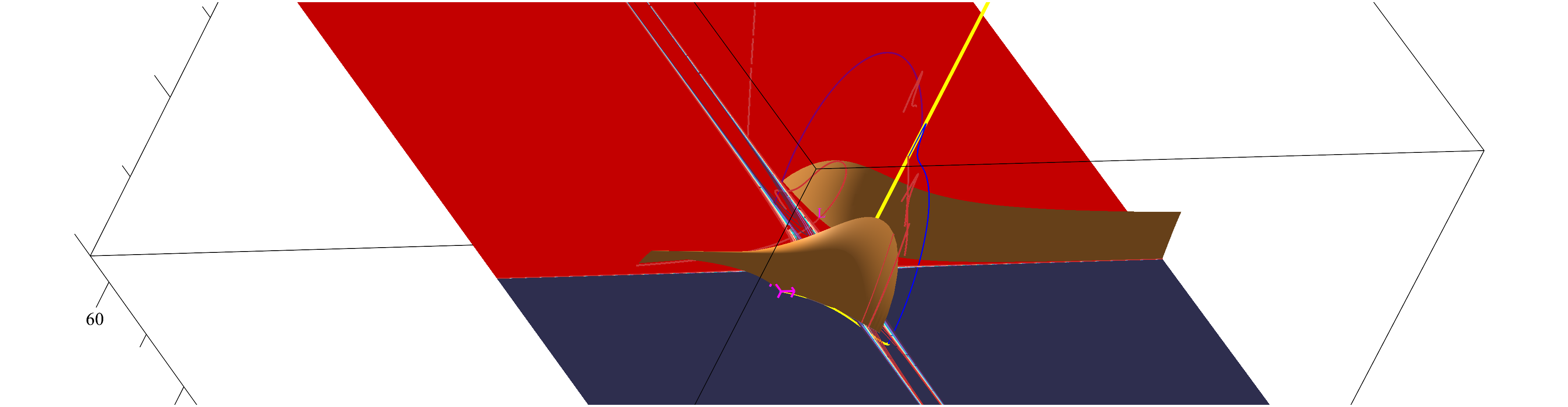
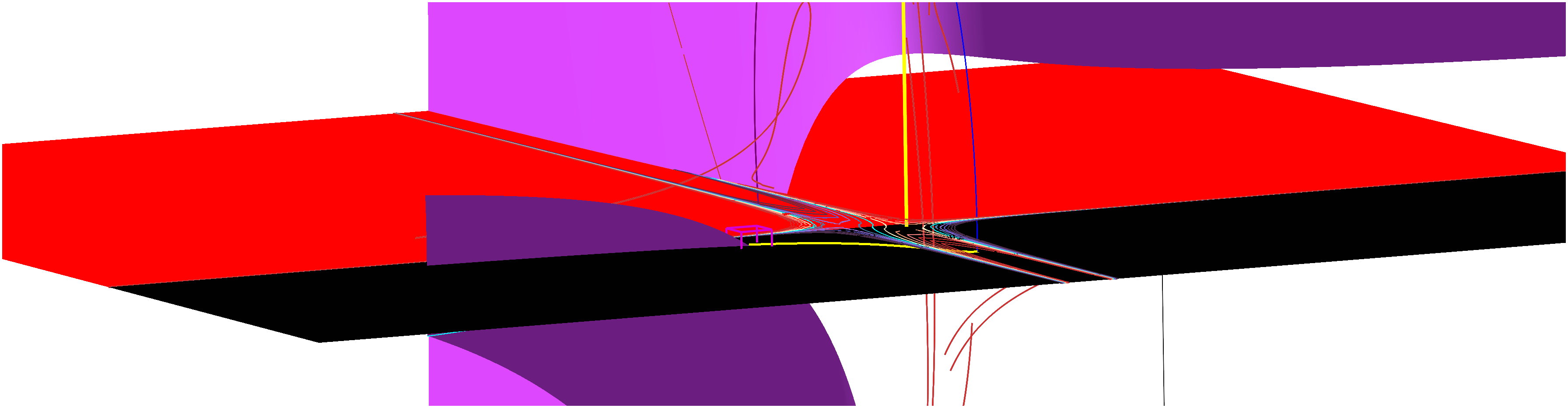
Refer to caption
Refer to caption
Figure 11: Left a:) The saturated of rarefaction wave. Right b:) The saturated of shock wave.
Refer to caption
Refer to caption
Figure 12: Left a:)The saturated of composite wave. Right b:) All saturated put together.

9.4 2-reverse wave sequence

To obtain the Riemann solution we need to construct the wave in the backward direction. We define the backward direction through 2-reverse shock. We will show that this 2-reverse shock, in following the direction from left to right is a Lax’s 2-shock, satisfying conditions (6.3), so, we define the rarefaction (and composite waves) in the opposite direction.

For a state U∈𝒞fU\in\mathcal{C}_{{}_{f}}, we define the 2-reverse shock as the arc of Hugoniot for which the shock speed increases along of this arc. The rarefaction is constructed in the opposite direction. Following this construction and remembering that Fig. , we have that the reverse rarefaction is drawn in the direction of ℐf\mathcal{I}_{{}_{f}} and the Hugoniot is drawn in the opposite direction as in Fig. 13.

Refer to caption
Figure 13: Direction of reverse waves in 𝒞f\mathcal{C}_{{}_{f}}.

We prove now that the reverse 2-shock satisfies the Lax’s condition (6.3).

First, we consider U~∈𝒞f\tilde{U}\in\mathcal{C}_{{}_{f}}. From U~\tilde{U} we draw the Hugoniot, that we denote as s​h​(U~)sh(\tilde{U}) and consider the arc for which shock speed increases as s​h+​(U)sh^{+}(U). Let U∈s​h+​(U~)U\in sh^{+}(\tilde{U}) and close to U~\tilde{U}. Notice that since we are constructing the reverse 2-shock, we have that for the direct wave U∈s​h+​(U~)U\in sh^{+}(\tilde{U}) represents the “left” state and U~\tilde{U} the “right”. Since the shock speed increasing ss in the reverse 2-shock, follows that

s(U)>s(U~)=λf(U),s(U)>s(\tilde{U})=\lambda_{{}_{f}}(U), (9.3)

that is the first inequality in (6.3).

To prove the other inequality of (6.3), we use the following assumption proved in [1]:

Assumption 9.1.

Let 𝒱∈𝒲\mathcal{V}\in\mathcal{W} be a neighborhood of a point 𝒰∈𝒞\mathcal{U}\in\mathcal{C} away from the inflection and the coincidence loci. Let 𝒱1\mathcal{V}_{{}_{1}} be one of the two connected components of 𝒱−𝒞\mathcal{V}-\mathcal{C}. In this paper we assume that if ss decreases along the Hugoniot curve through 𝒰\mathcal{U} into 𝒱1\mathcal{V}_{{}_{1}}, then ss increases along the Hugoniot′ curve through 𝒰\mathcal{U} into 𝒱1\mathcal{V}_{{}_{1}}. A similar statement is assumed to hold if ss increases along the Hugoniot curve into 𝒱1\mathcal{V}_{{}_{1}}.

Now, to prove the second inequality in (6.3), we need to obtain the projection of U∈s​h+​(U~)U\in sh^{+}(\tilde{U}) into 𝒞s\mathcal{C}_{{}_{s}} to obtain the values of λs\lambda_{{}_{s}} evaluated in these projetions. To do, we define Us{U}_{{}_{s}}, Uf{U}_{{}_{f}}, U′s{U^{\prime}}_{{}_{s}} and U′f{U^{\prime}}_{{}_{f}} to be the points satisfying (6.1)(\ref{usuli}). Notice that to reach U~\tilde{U} the shock speed decreases, thus, from the Assumption 9.1, the shock speed along of Hugoniot′ increases to reach UfU_{{}_{f}}, so, we know that

s(U)<s(Uf′)=λf(Uf′)s(U)<s(U^{\prime}_{{}_{f}})=\lambda_{{}_{f}}(U^{\prime}_{{}_{f}}) (9.4)

Finally, to reaches the projection U′sU^{\prime}_{{}_{s}}, we follows the opposite direction of the arc of Hugoniot′ that reaches U′fU^{\prime}_{{}_{f}}, thus the shock speed decreases along of this curve, so, we have that:

λs(U′)=s(U′)<s(U).\lambda_{{}_{s}}(U^{\prime})=s(U^{\prime})<s(U). (9.5)

Using (9.3), (9.4) and (9.5)(\ref{dds2}), we have that the shock satisfies the Lax’s condition (6.3) and it is a Lax’s 2-shock and the proof is completed.

Remark 7.

In [1], authors proved that the shock satisfies the Lax’s conditions, i.e., the shock is either 1-shock of Lax or a 2-shock of Lax. However, in the paper [1], to prove that the shock from for a state in CsC_{{}_{s}} is a 1-shock, authors consider U∈𝒞sU\in\mathcal{C}_{{}_{s}}, as a abuse in notation they consider another state that belongs to 1-shock curve that they also call as 𝒰\mathcal{U}. Despite the abuse of notation, they correctly proved that the shock is a 1-shock. A similar abuse of notation appears to consider that the 2-reverse shock is satisfies the Lax’s condition (6.3). In the present paper, we corrected these mistakes and we gave details of the proof that the 2-reverse shock satisfies the Lax’s conditions (6.3).

In the following examples we show the Riemann solution in the wave manifold 𝒲\mathcal{W} and the corresponding solution in u​vuv-plane.

9.5 Examples of solutions

Example 1.

First, we consider a state WL=(uL,vL)W_{{}_{L}}=(u_{{}_{L}},v_{{}_{L}}) for which the state 𝒰L\mathcal{U}_{{}_{L}} (obtained by Algorithm RS) belongs to II.

Applying the Algorithm RS, we construct the waves of family-1 through WLW_{{}_{L}}. For this example, we consider, see Fig 15.a.

In this example, we utilize zL=−5z_{{}_{L}}=-5 and tL=−0.065t_{{}_{L}}=-0.065 (the corresponding value in the u​vuv plane is uL=−0.2430769231u_{{}_{L}}=-0.2430769231 and vL=−0.6365384615v_{{}_{L}}=-0.6365384615). The sequence through 𝒰L\mathcal{U}_{{}_{L}} is ℋ1𝒰Lℛ1\mathcal{H}_{{}_{1}}\mathcal{U}_{{}_{L}}\mathcal{R}_{{}_{1}} and the curve stops at the coincidence curve. Notice that in this sequence, the rarefaction curve (ℛ1)(\mathcal{R}_{{}_{1}}) crosses 𝒞s\mathcal{C}_{{}_{s}} at t=0t=0, see Figs. 14 (in wave manifold 𝒲\mathcal{W}) and 15.a in the u​vuv-plane.

The saturated curves are described also in Fig. 14. The magenta surface is the saturated of ℋ1\mathcal{H}_{{}_{1}}; the brown surface is the saturated of ℛ1\mathcal{R}_{{}_{1}} and ℛ2\mathcal{R}_{{}_{2}}; the green surface is the saturated of 𝒞2\mathcal{C}_{{}_{2}}. The curve 𝒞2\mathcal{C}_{{}_{2}} is drawn to reach the double contact in z=1/3z=1/3.

Refer to caption
Refer to caption
Figure 14: The wave sequence and the saturated surface from 𝒰L\mathcal{U}_{{}_{L}} in region II, here zL=−5z_{{}_{L}}=-5 and tL=−0.065t_{{}_{L}}=-0.065. From 𝒰L\mathcal{U}_{{}_{L}}, denoted as a magenta box, we have the wave sequence ℋ1𝒰Lℛ1\mathcal{H}_{{}_{1}}\mathcal{U}_{{}_{L}}\mathcal{R}_{{}_{1}}. The magenta surface is the saturated of ℋ1\mathcal{H}_{{}_{1}}; the brown surface is the saturated of ℛ1\mathcal{R}_{{}_{1}} and ℛ2\mathcal{R}_{{}_{2}}; the green surface is the saturated of 𝒞2\mathcal{C}_{{}_{2}}. The curve 𝒞2\mathcal{C}_{{}_{2}} is drawn to reach the double contact in z=1/3z=1/3.
Refer to caption
Figure 15: The wave sequence on the plane u​vuv, here uL=−0.2430769231u_{{}_{L}}=-0.2430769231 and vL=−0.6365384615v_{{}_{L}}=-0.6365384615. From LL there is a ℋ1\mathcal{H}_{{}_{1}} (black curve) and a ℛ1\mathcal{R}_{{}_{1}} (red curve).

To construct the 2-reverse wave sequence, here we have two possibilities.

The first possibility, we give (zR=2,tR=2)∈𝒞f(z_{{}_{R}}=2,t_{{}_{R}}=2)\in\mathcal{C}_{{}_{f}} (the corresponding values on the plane u​vuv are (uR=0.8500000000,vR=3.200000000)(u_{{}_{R}}=0.8500000000,v_{{}_{R}}=3.200000000). From 𝒰r\mathcal{U}_{{}_{r}} (obtained as described in Algorithm RS) we draw the 2-reverse wave sequence that is given by ℋ2𝒰Rℛ2𝒞2\mathcal{H}_{{}_{2}}\mathcal{U}_{{}_{R}}\mathcal{R}_{{}_{2}}\mathcal{C}_{{}_{2}}, as described in Fig. 16. In the wave manifold 𝒲\mathcal{W}, ℛ2\mathcal{R}_{{}_{2}} is the green curve and 𝒞2\mathcal{C}_{{}_{2}} is the black curve, the ℋ2\mathcal{H}_{{}_{2}} is below 𝒞f\mathcal{C}_{{}_{f}}. Notice that, from Fig. 16.a, that 𝒞2\mathcal{C}_{{}_{2}} crosses the saturated of ℋ1\mathcal{H}_{{}_{1}} (the magenta surface) in a state in 𝒲\mathcal{W}.

The Riemann solution from state 𝒰L\mathcal{U}_{{}_{L}} consists of a ℋ1\mathcal{H}_{{}_{1}} from 𝒰L\mathcal{U}_{{}_{L}} to state 𝒰M\mathcal{U}_{{}_{M}}; from 𝒰M\mathcal{U}_{{}_{M}} there is a 𝒞2\mathcal{C}_{{}_{2}} (a right characteristic shock) followed by a ℛ2\mathcal{R}_{{}_{2}} to 𝒰R\mathcal{U}_{{}_{R}}. The solution in 𝒲\mathcal{W} is described in Fig. 16.a and in the u​vuv plane is described in 16.b.

Refer to caption
Figure 16: The Riemann solution from state 𝒰L\mathcal{U}_{{}_{L}} consists of a ℋ1\mathcal{H}_{{}_{1}} from 𝒰L\mathcal{U}_{{}_{L}} to state 𝒰M\mathcal{U}_{{}_{M}}; from 𝒰M\mathcal{U}_{{}_{M}} there is a 𝒞2\mathcal{C}_{{}_{2}} (a right characteristic shock) followed by a ℛ2\mathcal{R}_{{}_{2}} to 𝒰R\mathcal{U}_{{}_{R}}. Left- a:) The solution in the wave manifold 𝒲\mathcal{W}. Right- b:)The Riemann solution in plane u​vuv, for L=(uL=−0.2430769231,vL=−0.6365384615)L=(u_{{}_{L}}=-0.2430769231,v_{{}_{L}}=-0.6365384615) and R=(uR=−0.85,vR=3.2)R=(u_{{}_{R}}=-0.85,v_{{}_{R}}=3.2).

In the second possibility for 𝒰R\mathcal{U}_{{}_{R}}, we give (zR=0.385677655,tR=4.849940052)∈𝒞f(z_{{}_{R}}=0.385677655,t_{{}_{R}}=4.849940052)\in\mathcal{C}_{{}_{f}} (the corresponding values on the plane u​vuv are (uR=−0.6,vR=−1.1)(u_{{}_{R}}=-0.6,v_{{}_{R}}=-1.1). From 𝒰r\mathcal{U}_{{}_{r}} (obtained as described in Algorithm RS) we draw the 2-reverse wave sequence that is given by 𝒞2ℛ2𝒰Rℋ2\mathcal{C}_{{}_{2}}\mathcal{R}_{{}_{2}}\mathcal{U}_{{}_{R}}\mathcal{H}_{{}_{2}}, as described in Fig. 17. In the wave manifold 𝒲\mathcal{W}, ℛ2\mathcal{R}_{{}_{2}} is the green curve, ℋ2\mathcal{H}_{{}_{2}} is the blue curve and 𝒞2\mathcal{C}_{{}_{2}} is below 𝒞f\mathcal{C}_{{}_{f}}. Notice that, from Fig. 17.a, that ℛ2\mathcal{R}_{{}_{2}} crosses the saturated of ℋ1\mathcal{H}_{{}_{1}} (the magenta surface) in a state in 𝒲\mathcal{W}.

The Riemann solution from state 𝒰L\mathcal{U}_{{}_{L}} consists of a ℋ1\mathcal{H}_{{}_{1}} from 𝒰L\mathcal{U}_{{}_{L}} to state 𝒰M\mathcal{U}_{{}_{M}}; from 𝒰M\mathcal{U}_{{}_{M}} there is a ℛ2\mathcal{R}_{{}_{2}} to 𝒰R\mathcal{U}_{{}_{R}}. The solution in 𝒲\mathcal{W} is described in Fig. 17.a and in the u​vuv plane is described in 17.b.

Refer to caption
Figure 17: The 2-reverse wave sequence that is 𝒞2ℛ2𝒰Rℋ2\mathcal{C}_{{}_{2}}\mathcal{R}_{{}_{2}}\mathcal{U}_{{}_{R}}\mathcal{H}_{{}_{2}}. The Riemann solution from state 𝒰L\mathcal{U}_{{}_{L}} consists of a ℋ1\mathcal{H}_{{}_{1}} from 𝒰L\mathcal{U}_{{}_{L}} to state 𝒰M\mathcal{U}_{{}_{M}}; from 𝒰M\mathcal{U}_{{}_{M}} there is a ℛ2\mathcal{R}_{{}_{2}} to 𝒰R\mathcal{U}_{{}_{R}}. Left- a:) The solution in the wave manifold 𝒲\mathcal{W}, here ℛ2\mathcal{R}_{{}_{2}} is the green curve, ℋ2\mathcal{H}_{{}_{2}} is the blue curve and 𝒞2\mathcal{C}_{{}_{2}} is below 𝒞f\mathcal{C}_{{}_{f}}. Right- b:) The Riemann solution in plane u​vuv, for L=(uL=−0.2430769231,vL=−0.6365384615)L=(u_{{}_{L}}=-0.2430769231,v_{{}_{L}}=-0.6365384615) and R=(uR=−0.6,vR=−1.1)R=(u_{{}_{R}}=-0.6,v_{{}_{R}}=-1.1).

Example 2.

In this example we utilize zL=1z_{{}_{L}}=1 and tL=−1t_{{}_{L}}=-1 (the corresponding value in the u​vuv plane is uL=0.125,vL=0.5u_{{}_{L}}=0.125,v_{{}_{L}}=0.5), the state (zL,tL)(z_{{}_{L}},t_{{}_{L}}) belongs also to the region II. The sequence through 𝒰L\mathcal{U}_{{}_{L}} is ℋ1𝒰Lℛ1\mathcal{H}_{{}_{1}}\mathcal{U}_{{}_{L}}\mathcal{R}_{{}_{1}}, there is no composite wave because the rarefaction does not reach the inflection curve. However, notice that, the rarefaction curve (ℛ1)(\mathcal{R}_{{}_{1}}) crosses 𝒞s\mathcal{C}_{{}_{s}} at t=0t=0 and the wave curve stops, see Figs. 18 (in wave manifold 𝒲\mathcal{W}) and 19 in the u​vuv-plane.

The saturated curves are described also in Fig. 19. The magenta surface is the saturated of ℋ1\mathcal{H}_{{}_{1}}; the brown surface is the saturated of ℛ1\mathcal{R}_{{}_{1}} and ℛ2\mathcal{R}_{{}_{2}}.

Refer to caption
Refer to caption
Figure 18: The wave sequence and the saturated surface from 𝒰L\mathcal{U}_{{}_{L}} in region I​III, here zL=1z_{{}_{L}}=1 and tL=−1t_{{}_{L}}=-1. From 𝒰L\mathcal{U}_{{}_{L}}, denoted as a magenta box, we have the wave sequence ℋ1𝒰Lℛ1ℛ2\mathcal{H}_{{}_{1}}\mathcal{U}_{{}_{L}}\mathcal{R}_{{}_{1}}\mathcal{R}_{{}_{2}}. The magenta surface is the saturated of ℋ1\mathcal{H}_{{}_{1}} and the brown surface is the saturated of ℛ1\mathcal{R}_{{}_{1}} and ℛ2\mathcal{R}_{{}_{2}}; there is no composite wave, because the rarefaction does not reach the inflection curve. Here, we have different views of the 𝒰L\mathcal{U}_{{}_{L}}. Left- a:) The view for Y>0Y>0. Right- b:) The view with Y<0Y<0 the blue curve represents ℋ1\mathcal{H}_{{}_{1}} and yellow is ℛ1\mathcal{R}_{{}_{1}}.
Figure 19: The wave sequence on the plane u​vuv, here uL=0.125u_{{}_{L}}=0.125 and vL=0.5v_{{}_{L}}=0.5. From LL there is a ℋ1\mathcal{H}_{{}_{1}} (black curve) and a ℛ1\mathcal{R}_{{}_{1}} (red curve). The magenta ellipse is the elliptic region.

To construct the 2-reverse wave sequence, we consider 𝒰r\mathcal{U}_{{}_{r}} (obtained as described in Algorithm RS) and we draw the 2-reverse wave sequence that is given, in this example, by 𝒞2ℛ2𝒰Rℋ2\mathcal{C}_{{}_{2}}\mathcal{R}_{{}_{2}}\mathcal{U}_{{}_{R}}\mathcal{H}_{{}_{2}}, as described in Fig. 16. In the wave manifold 𝒲\mathcal{W}, ℛ2\mathcal{R}_{{}_{2}} is the green curve on the plane 𝒞f\mathcal{C}_{{}_{f}} and 𝒞2\mathcal{C}_{{}_{2}} is the black curve for Y<0Y<0 (below 𝒞f\mathcal{C}_{{}_{f}}, the ℋ2\mathcal{H}_{{}_{2}} is the blue curve for Y<0Y<0 (above 𝒞f\mathcal{C}_{{}_{f}}). Notice that, from Fig. 20.a, that 𝒞2\mathcal{C}_{{}_{2}} crosses the saturated of ℋ1\mathcal{H}_{{}_{1}} (the magenta surface) in a state in 𝒲\mathcal{W} for Y<0Y<0 (below 𝒞f\mathcal{C}_{{}_{f}}).

The Riemann solution from state 𝒰L\mathcal{U}_{{}_{L}} consists of a ℋ1\mathcal{H}_{{}_{1}} from 𝒰L\mathcal{U}_{{}_{L}} to state 𝒰M\mathcal{U}_{{}_{M}}; from 𝒰M\mathcal{U}_{{}_{M}} there is a 𝒞2\mathcal{C}_{{}_{2}} (a right characteristic shock) followed by a ℛ2\mathcal{R}_{{}_{2}} to 𝒰R\mathcal{U}_{{}_{R}}. The solution in 𝒲\mathcal{W} is described in Fig. 20 and in the u​vuv plane is described in Fig. 21.

Refer to caption
Refer to caption
Figure 20: The 2-reverse wave sequence that is 𝒞2ℛ2𝒰Rℋ2\mathcal{C}_{{}_{2}}\mathcal{R}_{{}_{2}}\mathcal{U}_{{}_{R}}\mathcal{H}_{{}_{2}}. The green curve on the plane 𝒞f\mathcal{C}_{{}_{f}} and 𝒞2\mathcal{C}_{{}_{2}} is the black curve for Y<0Y<0 (below 𝒞f\mathcal{C}_{{}_{f}}, the ℋ2\mathcal{H}_{{}_{2}} is the blue curve for Y<0Y<0 (above 𝒞f\mathcal{C}_{{}_{f}}). Notice that 𝒞2\mathcal{C}_{{}_{2}} crosses the saturated of ℋ1\mathcal{H}_{{}_{1}} (the magenta surface) in a state in 𝒲\mathcal{W} for Y<0Y<0 (below 𝒞f\mathcal{C}_{{}_{f}}).
Figure 21: The Riemann solution in plane u​vuv, for L=(uL=−0.125,vL=3.5)L=(u_{{}_{L}}=-0.125,v_{{}_{L}}=3.5) and R=(uR=−0.75,vR=−2.5)R=(u_{{}_{R}}=-0.75,v_{{}_{R}}=-2.5). From state LL consists of a ℋ1\mathcal{H}_{{}_{1}} from LL to state MM; from MM there is a 𝒞2\mathcal{C}_{{}_{2}} (a right characteristic shock) followed by a ℛ2\mathcal{R}_{{}_{2}} to RR.

Example 3.

In this example, we utilize zL=−1z_{{}_{L}}=-1 and tL=−4t_{{}_{L}}=-4 (the corresponding value in the u​vuv plane is uL=−0.125,vL=3.5u_{{}_{L}}=-0.125,v_{{}_{L}}=3.5), the state (zL,tL)(z_{{}_{L}},t_{{}_{L}}) belongs to the region I​III. The sequence through 𝒰L\mathcal{U}_{{}_{L}} is ℋ1𝒰Lℛ1𝒞1\mathcal{H}_{{}_{1}}\mathcal{U}_{{}_{L}}\mathcal{R}_{{}_{1}}\mathcal{C}_{{}_{1}}, see Figs. 22 (in wave manifold 𝒲\mathcal{W}) and 19 in the u​vuv-plane.

In Fig. 22, the magenta surface is the saturated of ℋ1\mathcal{H}_{{}_{1}}; the brown surface is the saturated of ℛ1\mathcal{R}_{{}_{1}} and ℛ2\mathcal{R}_{{}_{2}}; the green surface is the saturated of 𝒞2\mathcal{C}_{{}_{2}}. The curve 𝒞2\mathcal{C}_{{}_{2}} is drawn to reach the double contact in z=−1/3z=-1/3. In Fig. 23, the double contact z=−1/3z=-1/3 is the yellow straight line.

Refer to caption
Refer to caption
Figure 22: Here the values for 𝒰L\mathcal{U}_{{}_{L}} in I​I​IIII with zL=−1z_{{}_{L}}=-1 and tL=−4t_{{}_{L}}=-4. The sequence through 𝒰L\mathcal{U}_{{}_{L}} is ℋ1𝒰Lℛ1𝒞1\mathcal{H}_{{}_{1}}\mathcal{U}_{{}_{L}}\mathcal{R}_{{}_{1}}\mathcal{C}_{{}_{1}}. The magenta surface is the saturated of ℋ1\mathcal{H}_{{}_{1}} (blue curve); the brown surface is the saturated of ℛ1\mathcal{R}_{{}_{1}} (yellow curve); the green surface is the saturated of 𝒞2\mathcal{C}_{{}_{2}} (cyan). The curve 𝒞2\mathcal{C}_{{}_{2}} is drawn to reach the double contact in z=−1/3z=-1/3.
Figure 23: The wave sequence on the plane u​vuv, here uL=−0.125u_{{}_{L}}=-0.125 and vL=3.5v_{{}_{L}}=3.5. From LL there is a ℋ1\mathcal{H}_{{}_{1}} (black curve) and a ℛ1\mathcal{R}_{{}_{1}} (red curve), since the rarefaction crosses the inflection (blue curve), there is a 𝒞2\mathcal{C}_{{}_{2}} to the double contact (yellow straight line) z=−1/3z=-1/3. The magenta ellipse is the elliptic region.

To construct the 2-reverse wave sequence, here we consider (zR=5,tR=3)∈𝒞f(z_{{}_{R}}=5,t_{{}_{R}}=3)\in\mathcal{C}_{{}_{f}} (the corresponding values on the plane u​vuv are (uR=9.048076925,vR=14.03846154)(u_{{}_{R}}=9.048076925,v_{{}_{R}}=14.03846154). From 𝒰r\mathcal{U}_{{}_{r}} (obtained as described in Algorithm RS) we draw the 2-reverse wave sequence that is given, in this example, by ℋ2𝒰Rℛ2𝒞2\mathcal{H}_{{}_{2}}\mathcal{U}_{{}_{R}}\mathcal{R}_{{}_{2}}\mathcal{C}_{{}_{2}}, as described in Fig. 24. In the wave manifold 𝒲\mathcal{W}, ℛ2\mathcal{R}_{{}_{2}} is the green curve on 𝒞f\mathcal{C}_{{}_{f}}. The curve H1H_{{}_{1}} is drawn for Y<0Y<0, i.e., below 𝒞f\mathcal{C}_{{}_{f}} and 𝒞2\mathcal{C}_{{}_{2}} is the black curve behind the magenta surface (saturated of ℋ1\mathcal{H}_{{}_{1}}), from 𝒰R\mathcal{U}_{{}_{R}} there is only a wave crossing the magenta surface, that is ℛ2\mathcal{R}_{{}_{2}}.

In this case, the Riemann solution from state 𝒰L\mathcal{U}_{{}_{L}} consists of a ℋ1\mathcal{H}_{{}_{1}} from 𝒰L\mathcal{U}_{{}_{L}} to state 𝒰M\mathcal{U}_{{}_{M}}; from 𝒰M\mathcal{U}_{{}_{M}} there is a ℛ2\mathcal{R}_{{}_{2}} to 𝒰R\mathcal{U}_{{}_{R}}. The solution in 𝒲\mathcal{W} is described in Fig. 24 and in the u​vuv plane is described in 25.

Refer to caption
Refer to caption
Figure 24: The 2-reverse wave sequence for (zR=5,tR=3)∈𝒞f(z_{{}_{R}}=5,t_{{}_{R}}=3)\in\mathcal{C}_{{}_{f}} is ℋ2𝒰Rℛ2𝒞2\mathcal{H}_{{}_{2}}\mathcal{U}_{{}_{R}}\mathcal{R}_{{}_{2}}\mathcal{C}_{{}_{2}}. The ℛ2\mathcal{R}_{{}_{2}} is the green curve on 𝒞f\mathcal{C}_{{}_{f}}. The curve H1H_{{}_{1}} is drawn for Y<0Y<0 (below 𝒞f\mathcal{C}_{{}_{f}}) and 𝒞2\mathcal{C}_{{}_{2}} is the black curve behind the magenta surface. The Riemann solution from state 𝒰L\mathcal{U}_{{}_{L}} consists of a ℋ1\mathcal{H}_{{}_{1}} from 𝒰L\mathcal{U}_{{}_{L}} to state 𝒰M\mathcal{U}_{{}_{M}}; from 𝒰M\mathcal{U}_{{}_{M}} there is a ℛ2\mathcal{R}_{{}_{2}} to 𝒰R\mathcal{U}_{{}_{R}}.
Figure 25: The Riemann solution in plane u​vuv, for L=(uL=−0.125,vL=3.5)L=(u_{{}_{L}}=-0.125,v_{{}_{L}}=3.5) and R=(uR=9.048076925,vR=14.03846154)R=(u_{{}_{R}}=9.048076925,v_{{}_{R}}=14.03846154). From LL there is a ℋ1\mathcal{H}_{{}_{1}} to a state MM (black curve); from MM there is a ℛ2\mathcal{R}_{{}_{2}} (pink curve) to RR.The blue curve is the inflection.

Example 4.

In this example, we utilize zL=1z_{{}_{L}}=1 and tL=−2t_{{}_{L}}=-2 (the corresponding value in the u​vuv plane is uL=0.125,vL=−2.5u_{{}_{L}}=0.125,v_{{}_{L}}=-2.5), the state (zL,tL)(z_{{}_{L}},t_{{}_{L}}) belongs to the region I​I​IIII. The sequence through 𝒰L\mathcal{U}_{{}_{L}} is 𝒞1ℛ1𝒰Lℋ1\mathcal{C}_{{}_{1}}\mathcal{R}_{{}_{1}}\mathcal{U}_{{}_{L}}\mathcal{H}_{{}_{1}}, see Figs. 26 (in wave manifold 𝒲\mathcal{W}) and 27 (in the u​vuv-plane).

In Fig. 26, the magenta surface is the saturated of ℋ1\mathcal{H}_{{}_{1}}; the brown surface is the saturated of ℛ1\mathcal{R}_{{}_{1}} and ℛ2\mathcal{R}_{{}_{2}}; the green surface is the saturated of 𝒞2\mathcal{C}_{{}_{2}}. The curve 𝒞2\mathcal{C}_{{}_{2}} is drawn to reach the double contact in z=1/3z=1/3 (with t<0t<0). In Fig. 27, the double contact z=1/3z=1/3 is the purple straight line.

Refer to caption
Refer to caption
Figure 26: Here the values for 𝒰L\mathcal{U}_{{}_{L}} in I​I​IIII with zL=1z_{{}_{L}}=1 and tL=−2t_{{}_{L}}=-2. The sequence through 𝒰L\mathcal{U}_{{}_{L}} is 𝒞1ℛ1𝒰Lℋ1\mathcal{C}_{{1}}\mathcal{R}_{{}_{1}}\mathcal{U}_{{}_{L}}\mathcal{H}_{{}_{1}}. The magenta surface is the saturated of ℋ1\mathcal{H}_{{}_{1}} (blue curve); the brown surface is the saturated of ℛ1\mathcal{R}_{{}_{1}} (yellow curve); the green surface is the saturated of 𝒞2\mathcal{C}_{{}_{2}} (cyan). The curve 𝒞2\mathcal{C}_{{}_{2}} is drawn to reach the double contact in z=1/3z=1/3.
Figure 27: The wave sequence on the plane u​vuv, here uL=0.125u_{{}_{L}}=0.125 and vL=−2.5v_{{}_{L}}=-2.5. From LL there is a ℋ1\mathcal{H}_{{}_{1}} (black curve) and a ℛ1\mathcal{R}_{{}_{1}} (red curve), since the rarefaction crosses the inflection (blue curve), there is a 𝒞2\mathcal{C}_{{}_{2}} to the double contact (purple straight line) z=1/3z=1/3. The magenta ellipse is the elliptic region.

To construct the 2-reverse wave sequence, here we consider (zR=4.961249694,tR=1)∈𝒞f(z_{{}_{R}}=4.961249694,t_{{}_{R}}=1)\in\mathcal{C}_{{}_{f}} (the corresponding values on the plane u​vuv are (uR=3,vR=4)(u_{{}_{R}}=3,v_{{}_{R}}=4). From 𝒰r\mathcal{U}_{{}_{r}} (obtained as described in Algorithm RS) we draw the 2-reverse wave sequence that is given, in this example, by 𝒞2ℛ2𝒰Rℋ2\mathcal{C}_{{}_{2}}\mathcal{R}_{{}_{2}}\mathcal{U}_{{}_{R}}\mathcal{H}_{{}_{2}}, as described in Fig. 28. In the wave manifold 𝒲\mathcal{W}, ℛ2\mathcal{R}_{{}_{2}} is the green curve on 𝒞f\mathcal{C}_{{}_{f}}. The curve H1H_{{}_{1}} is the cyan curve drawn for Y>0Y>0 and increasing zz. The curve 𝒞2\mathcal{C}_{{}_{2}} is the black curve below 𝒞f\mathcal{C}_{{}_{f}}, from 𝒰R\mathcal{U}_{{}_{R}} the curve ℛ2\mathcal{R}_{{}_{2}} crosses the saturated surface of 𝒞1\mathcal{C}_{{}_{1}} (green surface).

In this case, the Riemann solution from state 𝒰L\mathcal{U}_{{}_{L}} consists of a ℛ1\mathcal{R}_{{}_{1}} followed by a 𝒞1\mathcal{C}_{{}_{1}} to a state 𝒰M\mathcal{U}_{{}_{M}}; from 𝒰M\mathcal{U}_{{}_{M}} there is a ℛ2\mathcal{R}_{{}_{2}} to 𝒰R\mathcal{U}_{{}_{R}}. The solution in 𝒲\mathcal{W} is described in Fig. 28 and in the u​vuv plane is described in Fig. 29.

Refer to caption
Refer to caption
Figure 28: The 2-reverse wave sequence for (zR=4.961249694,tR=1)∈𝒞f(z_{{}_{R}}=4.961249694,t_{{}_{R}}=1)\in\mathcal{C}_{{}_{f}} is 𝒞2ℛ2𝒰Rℋ2\mathcal{C}_{{}_{2}}\mathcal{R}_{{}_{2}}\mathcal{U}_{{}_{R}}\mathcal{H}_{{}_{2}}. Here ℛ2\mathcal{R}_{{}_{2}} is the green curve on 𝒞f\mathcal{C}_{{}_{f}}. The curve H1H_{{}_{1}} is the cyan curve drawn for Y>0Y>0 and increasing zz. The curve 𝒞2\mathcal{C}_{{}_{2}} is the black curve below 𝒞f\mathcal{C}_{{}_{f}}, from 𝒰R\mathcal{U}_{{}_{R}} the curve ℛ2\mathcal{R}_{{}_{2}} crosses the saturated surface of 𝒞1\mathcal{C}_{{}_{1}} (green surface). The Riemann solution from state 𝒰L\mathcal{U}_{{}_{L}} consists of a ℛ1\mathcal{R}_{{}_{1}} followed by a 𝒞1\mathcal{C}_{{}_{1}} to a state 𝒰M\mathcal{U}_{{}_{M}}; from 𝒰M\mathcal{U}_{{}_{M}} there is a ℛ2\mathcal{R}_{{}_{2}} to 𝒰R\mathcal{U}_{{}_{R}}.
Figure 29: The Riemann solution in plane u​vuv, for L=(uL=0.125,vL=−2.5)L=(u_{{}_{L}}=0.125,v_{{}_{L}}=-2.5) and R=(uR=3,vR=4)R=(u_{{}_{R}}=3,v_{{}_{R}}=4). From LL there is a ℛ1\mathcal{R}_{{}_{1}} (red curve) followed by a 𝒞1\mathcal{C}_{{}_{1}} (green curve) to state MM (black curve); from MM there is a ℛ2\mathcal{R}_{{}_{2}} (pink curve) to RR.The blue curve is the inflection. The purple is the double contact that corresponds to z=1/3z=1/3.

9.6 The Regions in Phase Space

For the flux function f⁡(u,v)f(u,v) and g⁡(u,v)g(u,v) given in equation (2.1)(\ref{fgeq}), we can obtain the eigenpairs (eigenvalues, λ\lambda, and eigenvectors, 𝒓→\vec{\boldsymbol{r}}) in the phase space (u,v)(u,v). These eigenpairs are solutions of:

𝐀​𝒓→=λ​𝒓→, where ​λ​ is obtained solving ​det⁡(𝐀−λ​𝐈)=0.\mathbf{A}\vec{\boldsymbol{r}}=\lambda\vec{\boldsymbol{r}},\quad\text{ where }\ \lambda\ \text{ is obtained solving }\ \operatorname{det}(\mathbf{A}-\lambda\mathbf{I})=0. (9.6)

Here 𝐀\mathbf{A} is the jacobian of (f,g)T(f,g)^{{}^{\mathrm{T}}} and 𝐈\mathbf{I} is the 2×22\times 2 identity matrix. Notice that from equation (9.6.b)(\ref{eqts}.b) we have a degree two polynomial, thus for each state (u,v)(u,v) in the phase space we have associated two eigenvalues λ\lambda. The phase space is classified using λ\lambda and 𝒓→\vec{\boldsymbol{r}}. The region in the phase space (u,v)(u,v) for which each state admits two real eigenvalues λ\lambda and a basis of eigenvectors (local) is called hyperbolic region, which we denote as ℛH\mathcal{R}_{{}_{H}}. The region for which we have complex (and conjugated) eigenvalues λ\lambda is called elliptic region, denoted as ℛE\mathcal{R}_{{}_{E}}. The boundary (if this boundary exits) between ℛH\mathcal{R}_{{}_{H}} and ℛE\mathcal{R}_{{}_{E}} is denoted as ∂ℛE\partial\mathcal{R}_{{}_{E}}, here the two eigenvalues are equals.

For f⁡(u,v)f(u,v) and g⁡(u,v)g(u,v) given in equation (2.1) the eigenvalues are:

λ1=α1−α22 and λ2=α1+α22, where α1=u(b1+2)+a1+a4and\displaystyle\lambda_{{}_{1}}=\frac{\alpha_{{}_{1}}-\sqrt{\alpha_{{}_{2}}}}{2}\quad\text{ and }\quad\lambda_{{}_{2}}=\frac{\alpha_{{}_{1}}+\sqrt{\alpha_{{}_{2}}}}{2},\quad\text{ where }\alpha_{{}_{1}}=u(b_{{}_{1}}+2)+a_{{}_{1}}+a_{{}_{4}}\quad\text{and} (9.7)
α2=a12+(2b1u−2a4)a1+a42−2a4b1u+b12u2+4(v+a2)(a3+v)\displaystyle\alpha_{{}_{2}}=a_{{}_{1}}^{{}^{2}}+(2b_{{}_{1}}u-2a_{{}_{4}})a_{{}_{1}}+a_{{}_{4}}^{{}^{2}}-2a_{{}_{4}}b_{{}_{1}}u+b_{{}_{1}}^{{}^{2}}u^{{}^{2}}+4(v+a_{{}_{2}})(a_{{}_{3}}+v) (9.8)

To obtain ℛH\mathcal{R}_{{}_{H}}, ℛE\mathcal{R}_{{}_{E}} and ∂ℛE\partial\mathcal{R}_{{}_{E}}, we need to study the signal of α2\alpha_{{}_{2}}. After some algebraic, we can write α2\alpha_{{}_{2}} and define α~2\widetilde{\alpha}_{{}_{2}} as:

α2=(2v+a2+a3)2+(b1u+a1−a4)2−c2,α~2=[v+a2+a32]2(c2)2+[u+a1−a4b1]2(cb1)2−1.\alpha_{{}_{2}}=(2v+a_{{}_{2}}+a_{{}_{3}})^{{}^{2}}+(b_{{}_{1}}u+a_{{}_{1}}-a_{{}_{4}})^{{}^{2}}-c^{{}^{2}},\quad\widetilde{\alpha}_{{}_{2}}=\frac{[v+\frac{a_{{}_{2}}+a_{{}_{3}}}{2}]^{{}^{2}}}{(\frac{c}{2})^{{}^{2}}}+\frac{[u+\frac{a_{{}_{1}}-a_{{}_{4}}}{b_{{}_{1}}}]^{{}^{2}}}{(\frac{c}{b_{{}_{1}}})^{{}^{2}}}-1. (9.9)

Here, we use that c=a3−a2>0c=a_{{}_{3}}-a_{{}_{2}}>0. From α~2\widetilde{\alpha}_{{}_{2}}, we can define:

ℛH={(u,v)/α~2>0},ℛE={(u,v)/α~2<0} and ∂ℛE={(u,v)/α~2=0}.\displaystyle\mathcal{R}_{{}_{H}}=\{(u,v)\;/\;\widetilde{\alpha}_{{}_{2}}>0\},\;\mathcal{R}_{{}_{E}}=\{(u,v)\;/\;\widetilde{\alpha}_{{}_{2}}<0\}\text{ and }\partial\mathcal{R}_{{}_{E}}=\{(u,v)\;/\;\widetilde{\alpha}_{{}_{2}}=0\}. (9.10)

Notice that ∂ℛE\partial\mathcal{R}_{{}_{E}} represents an ellipse. In Fig. 30.a, we illustrate ℛH\mathcal{R}_{{}_{H}}, ℛE\mathcal{R}_{{}_{E}} and ∂ℛE\partial\mathcal{R}_{{}_{E}} for particular values of a1a_{{}_{1}}, a2a_{{}_{2}}, a3a_{{}_{3}}, a4a_{{}_{4}}, cc and b1b_{{}_{1}} described in caption of figure.

Refer to caption
Figure 30: Left - a:). Regions ℛE\mathcal{R}_{{}_{E}}, ℛH\mathcal{R}_{{}_{H}} and the boundary ∂ℛE\partial\mathcal{R}_{{}_{E}}. Here we use a1=0a_{{}_{1}}=0, a2=0a_{{}_{2}}=0, a3=1a_{{}_{3}}=1, a4=0a_{{}_{4}}=0, c=1c=1, and b1=8b_{{}_{1}}=8.

From the variables change defined Section 2, we obtain uu, vv, u′u^{\prime} and v′v^{\prime} as function of YY, tt and zz. The variables uu and vv are:

u=2t(z4−1)+Yb1z3+(−2a1+2a4)(z2+1)+(Yb1+4c)z2(z2+1)b1,\displaystyle u=\frac{2t(z^{{}^{4}}-1)+Yb_{{}_{1}}z^{{}^{3}}+(-2a_{{}_{1}}+2a_{{}_{4}})(z^{{}^{2}}+1)+(Yb_{{}_{1}}+4c)z}{2(z^{{}^{2}}+1)b_{{}_{1}}}, (9.11)
v=2tz3+(Y−2a3)z2+2tz+Y−2a22z2+2\displaystyle v=\frac{2tz^{{}^{3}}+(Y-2a_{{}_{3}})z^{{}^{2}}+2tz+Y-2a_{{}_{2}}}{2z^{{}^{2}}+2} (9.13)

to obtain u′u^{\prime} and v′v^{\prime} we use uu and vv interchanging YY with −Y-Y.

Substituting in α2\alpha_{{}_{2}}, uu and vv given equations (9.11), (9.13), we obtain an expression that we denote as αM(Y,t,z)\alpha_{{}_{M}}(Y,t,z):

αM(Y,t,z)\displaystyle\alpha_{{}_{M}}(Y,t,z) =\displaystyle= (Y2b12+12t2)z4+16Ytz3+[(b12+4)Y2+8c(b1−1)Y+4c2+12t2−4c]z24z2+4\displaystyle\frac{(Y^{{}^{2}}b_{{}_{1}}^{{}^{2}}+12t^{{}^{2}})z^{{}^{4}}+16Ytz^{{}^{3}}+[(b_{{}_{1}}^{{}^{2}}+4)Y^{{}^{2}}+8c(b_{{}_{1}}-1)Y+4c^{{}^{2}}+12t^{{}^{2}}-4c]z^{{}^{2}}}{4z^{{}^{2}}+4} (9.14)
+4t2z6+4Yb1tz5−4t(b1−4)Yz+4Y2+8Yc+4c2+4t2−4c4z2+4.\displaystyle+\frac{4t^{{}^{2}}z^{{}^{6}}+4Yb_{{}_{1}}tz^{{}^{5}}-4t(b_{{}_{1}}-4)Yz+4Y^{{}^{2}}+8Yc+4c^{{}^{2}}+4t^{{}^{2}}-4c}{4z^{{}^{2}}+4}.

If we set αM=0\alpha_{{}_{M}}=0, we obtain the extension of ℛE\mathcal{R}_{{}_{E}} in 𝒲\mathcal{W}, which we will call coincidence surface, i.e.,

coincidence={(z,t,Y)/αM=0}.coincidence=\{(z,t,Y)\;/\;\alpha_{{}_{M}}=0\}. (9.15)

Similarly, we define coincidence′ that is obtained substituting u′u^{\prime} and v′v^{\prime} in α2\alpha_{{}_{2}}. This expression is denoted as αM′=αM(z,t,−Y)\alpha_{{}_{M}}^{\prime}=\alpha_{{}_{M}}(z,t,-Y), thus coincidence′={(z,t,Y)/αM′=0}coincidence^{\prime}=\{(z,t,Y)\;/\;\alpha_{{}_{M}}^{\prime}=0\}. In Fig. 31, we show coincidence surface and the characteristic 𝒞\mathcal{C}. The coincidence′ surface is the symmetric projection of the coincidence surface in 𝒞\mathcal{C}.

Refer to caption
Figure 31: Left - a:). Regions ℛE\mathcal{R}_{{}_{E}}, ℛH\mathcal{R}_{{}_{H}} and the boundary ∂ℛE\partial\mathcal{R}_{{}_{E}}. Here, we use a1=0a_{{}_{1}}=0, a2=0a_{{}_{2}}=0, a3=1a_{{}_{3}}=1, a4=0a_{{}_{4}}=0, c=1c=1, and b1=8b_{{}_{1}}=8.

Appendix

1 Characterizing the L2 Condition

In this appendix section, we will prove that the necessary and sufficient condition to verify the condition L2 is that z2<1/(b1+1).z^{{}^{2}}<1/(b_{{}_{1}}+1).

As in Section 2.1, parametric equations for the Hugoniot′ curve through a point (t0,z0,Y0)(t_{{}_{0}},z_{{}_{0}},Y_{{}_{0}}) is given by

{Y=A′z2+B′z+C′(z02+1)[(b1−1)z2+1]t=D′z3+E′z2+F′z+G′c(z02+1)[(b1−1)z4+b1z2+1],\left\{\begin{array}[]{l}Y=\displaystyle\frac{A^{\prime}z^{{}^{2}}+B^{\prime}z+C^{\prime}}{(z_{{}_{0}}^{{}^{2}}+1)[(b_{{}_{1}}-1)z^{{}^{2}}+1]}\\ \\ t=\displaystyle\frac{D^{\prime}z^{{}^{3}}+E^{\prime}z^{{}^{2}}+F^{\prime}z+G^{\prime}}{c(z_{{}_{0}}^{{}^{2}}+1)[(b_{{}_{1}}-1)z^{{}^{4}}+b_{{}_{1}}z^{{}^{2}}+1]},\end{array}\right. (1.1)

where A′A^{\prime}, B′B^{\prime}, C′C^{\prime}, D′D^{\prime}, E′E^{\prime}, F′F^{\prime}, G′G^{\prime} are obtained from equations (2.12) by changing YY into −Y-Y and Y0Y_{{}_{0}} into −Y0-Y_{{}_{0}}.

Parametric equations for Hugoniot′ curve through a point of S​o​n′Son^{\prime} are obtained from the equations (1.1) substituting t0t_{{}_{0}} by t′0t^{\prime}_{{}_{0}}, t′0t^{\prime}_{{}_{0}} as in Section 5, getting (Yh​u​g′(z),th​u​g′(z))(Y_{{}_{hug^{\prime}}}(z),t_{{}_{hug^{\prime}}}(z)).

We need to calculate the speed ss at the intersections points of the Hugoniot′ curve with 𝒞\mathcal{C} and then write the condition L2. As the inequalities involved change only in S​o​nSon, it is enough to verify them at a point of S​o​n′Son^{\prime}. The speed ss at the point (t0′,z0,Y0)(t^{\prime}_{{}_{0}},z_{{}_{0}},Y_{{}_{0}}) is given by the equation (5.1).

Let z1z_{{}_{1}} and z2z_{{}_{2}} be, z1<z2z_{{}_{1}}<z_{{}_{2}}, the solutions of the equation Yh​u​g′=0Y_{{}_{hug^{\prime}}}=0. The roots z1z_{{}_{1}} and z2z_{{}_{2}} are the zz coordinates of the intersection points of the Hugoniot′ curve with 𝒞\mathcal{C}. The speed, sh​u​g′(z)s_{{}_{hug^{\prime}}}(z), along the Hugoniot′ curve through (t0′,z0,Y0)(t^{\prime}_{{}_{0}},z_{{}_{0}},Y_{{}_{0}}) is obtained by changing tt into th​u​g′(z)t_{{}_{hug^{\prime}}}(z) in equation (2.9). We must compare the values sh​u​g′(z1)s_{{}_{hug^{\prime}}}(z_{{}_{1}}) and sh​u​g′(z2)s_{{}_{hug^{\prime}}}(z_{{}_{2}}) with ss​o​n′s_{{}_{son^{\prime}}}. Denoting by sh​u​g′​n(z)s_{{}_{hug^{\prime}n}}(z) the numerator of sh​u​g′(z)s_{{}_{hug^{\prime}}}(z), sh​u​g′​d(z)s_{{}_{hug^{\prime}d}}(z) the denominator of sh​u​g′(z)s_{{}_{hug^{\prime}}}(z) and Yh​u​g′​n(z)Y_{{}_{hug^{\prime}n}}(z) the numerator of Yh​u​g′(z)Y_{{}_{hug^{\prime}}}(z), we can write

sh​u​g′​n(z)=p1(z)Yh​u​g′​n(z)+r1(z)s_{{}_{hug^{\prime}n}}(z)=p_{{}_{1}}(z)Y_{{}_{hug^{\prime}n}}(z)+r_{{}_{1}}(z)

and

sh​u​g′​d(z)=p2(z)Yh​u​g′​n(z)+r2(z).s_{{}_{hug^{\prime}d}}(z)=p_{{}_{2}}(z)Y_{{}_{hug^{\prime}n}}(z)+r_{{}_{2}}(z).

It follows that, sh​u​g′​𝒞(z)s_{{}_{hug^{\prime}\mathcal{C}}}(z), given by

sh​u​g′​𝒞(z)=r1(z)r2(z),s_{{}_{hug^{\prime}\mathcal{C}}}(z)=\frac{r_{{}_{1}}(z)}{r_{{}_{2}}(z)},

has the same value of sh​u​g′(z)s_{{}_{hug^{\prime}}}(z) at the intersection points of the Hugoniot′ curve through (t0′,z0,Y0)(t^{\prime}_{{}_{0}},z_{{}_{0}},Y_{{}_{0}}) with 𝒞\mathcal{C}. The expression of sh​u​g′​𝒞(z)s_{{}_{hug^{\prime}\mathcal{C}}}(z) is of the form (a​z+b)/(c​z+d)(az+b)/(cz+d). Our goal is to get a condition such that ss​o​n′(t0′,z0.Y0)s_{{}_{son^{\prime}}}(t^{\prime}_{{}_{0}},z_{{}_{0}}.Y_{{}_{0}}) satisfies sh​u​g′​𝒞(z1)<ss​o​n′(t0′,z0.Y0)<sh​u​g′​𝒞(z2)s_{{}_{hug^{\prime}\mathcal{C}}}(z_{{}_{1}})<s_{{}_{son^{\prime}}}(t^{\prime}_{{}_{0}},z_{{}_{0}}.Y_{{}_{0}})<s_{{}_{hug^{\prime}\mathcal{C}}}(z_{{}_{2}}).

In a more general way, we have the following problem: given a number ss we want a condition such that

az1+bcz1+d<s<az2+bcz2+d,\frac{az_{{}_{1}}+b}{cz_{{}_{1}}+d}<s<\frac{az_{{}_{2}}+b}{cz_{{}_{2}}+d},

where z1z_{{}_{1}} and z2z_{{}_{2}} are the roots of the polynomial fz2+gz+hfz^{{}^{2}}+gz+h. Straightforward computations give that the condition is

(c2h−dcg+d2f)s2+[agd+bcg−2(ach+bdf)]s+a2h−abg+b2fc2h−dcg+d2f<0.\frac{(c^{{}^{2}}h-dcg+d^{{}^{2}}f)s^{{}^{2}}+[agd+bcg-2(ach+bdf)]s+a^{{}^{2}}h-abg+b^{{}^{2}}f}{c^{{}^{2}}h-dcg+d^{{}^{2}}f}<0.

Changing aa, bb into the coefficients of the numerator of sh​u​g′​𝒞(z)s_{{}_{hug^{\prime}\mathcal{C}}}(z), cc and dd into the coefficients of the denominator of sh​u​g′​𝒞(z)s_{{}_{hug^{\prime}\mathcal{C}}}(z) and ff, gg, hh into the coefficients of the numerator of Yh​u​g′(z)Y_{{}_{hug^{\prime}}}(z), we get that the condition is

c​o​n​d=Y02((b1+1)z02−12<0,cond=\frac{Y_{{}_{0}}^{{}^{2}}((b_{{}_{1}}+1)z_{{}_{0}}^{{}^{2}}-1}{2}<0,

it follows that the condition L2 is satisfied if and only if −1/b1+1<z<1/b1+1.-1/\sqrt{b_{{}_{1}}+1}<z<1/\sqrt{b_{{}_{1}}+1}.

2 Lax’s inequalities in the wave manifold

The Lax’s inequalities for shocks are used to select shock (entropy condition) and used to prove uniqueness in the solution.

For a 22 system of equations (1.1), we have a pair of inequalities associated to a 1-shock and another pair of inequalities associated to a 2-shock.

In the Lax’s theory, the system is strictly hyperbolic with two different eigenvalues λ1(W)<λ2(W)\lambda_{{}_{1}}(W)<\lambda_{{}_{2}}(W). For regions for which the solution is continuous, we can define the ii-characteristic on the plane x​txt, for i=1,2i=1,2, solving:

d​xd​t=λi(W).\frac{dx}{dt}=\lambda_{{}_{i}}(W). (2.1)

For a shock between a state W−=(u−,v−)W^{-}=(u^{-},v^{-}) to W+=(u+,v+)W^{+}=(u^{+},v^{+}), with shock speed s⁡(W−,W+)s(W^{-},W^{+}), the 1-shock satisfies the inequalities given by:

s(W−,W+)<λ1(W−) and λ1(W+)<s(W−,W+)<λ2(W+).s(W^{-},W^{+})<\lambda_{{}_{1}}(W^{-})\quad\text{ and }\quad\lambda_{{}_{1}}(W^{+})<s(W^{-},W^{+})<\lambda_{{}_{2}}(W^{+}). (2.2)

The condition (2.2) states that the 1-characteristic wave, on the plane x​txt, (of each side of the shock) enter in the shock wave (with slope ss).

The 2-shock satisfies the inequalities given by:

s(W−,W+)>λ2(W+) and λ1(W−)<s(W−,W+)<λ2(W−).s(W^{-},W^{+})>\lambda_{{}_{2}}(W^{+})\quad\text{ and }\quad\lambda_{{}_{1}}(W^{-})<s(W^{-},W^{+})<\lambda_{{}_{2}}(W^{-}). (2.3)

The condition (2.3) states that the 2-characteristic wave, on the plane x​txt, (of each side of the shock) enter in the shock wave (with slope ss).

Here, we describe the Lax inequalities in the wave manifold.

For a state 𝒰∈𝒲\mathcal{U}\in\mathcal{W}, using the Hugoniot′, we obtain the projections 𝒰′s∈𝒞s\mathcal{U}^{\prime}_{{}_{s}}\in\mathcal{C}_{{}_{s}} and 𝒰′f∈𝒞f\mathcal{U}^{\prime}_{{}_{f}}\in\mathcal{C}_{{}_{f}}, using Eq. (6.1). So, we have that the eigenvalue associated to λ1\lambda_{{}_{1}} in the wave manifold is λs\lambda_{{}_{s}} and the eigenvalue associated to λ2\lambda_{{}_{2}} in the wave manifold is λf\lambda_{{}_{f}}. We consider another 𝒰~∈s​h​(𝒰)\widetilde{\mathcal{U}}\in sh(\mathcal{U}), whose projections in 𝒞s\mathcal{C}_{{}_{s}} and 𝒞f\mathcal{C}_{{}_{f}} are, respectivelly, 𝒰~′s\widetilde{\mathcal{U}}^{\prime}_{{}_{s}} and 𝒰~′f\widetilde{\mathcal{U}}^{\prime}_{{}_{f}}.

Using the previous analysis, the 1-shock in the wave manifold between the states 𝒰∈𝒲\mathcal{U}\in\mathcal{W} and 𝒰~∈s​h​(𝒰)\widetilde{\mathcal{U}}\in sh(\mathcal{U}) becomes:

s(𝒰~)<=s(𝒰s′)=λs(𝒰s′) and λs(𝒰~′)=s(𝒰~s′)<s(𝒰~)<s(𝒰~f′)=λf(𝒰~f′).s(\widetilde{\mathcal{U}})<=s(\mathcal{U}_{{}_{s}}^{\prime})=\lambda_{{}_{s}}(\mathcal{U}^{\prime}_{{}_{s}})\quad\text{ and }\quad\lambda_{{}_{s}}(\widetilde{\mathcal{U}}^{\prime})=s(\widetilde{\mathcal{U}}^{\prime}_{{}_{s}})<s(\widetilde{\mathcal{U}})<s(\widetilde{\mathcal{U}}^{\prime}_{{}_{f}})=\lambda_{{}_{f}}(\widetilde{\mathcal{U}}_{{}_{f}}^{\prime}). (2.4)

Here, we use that the shock speed ss equals to the λ\lambda in 𝒞\mathcal{C}.

The 2-shock in the wave manifold between the states 𝒰∈𝒲\mathcal{U}\in\mathcal{W} and 𝒰~∈s​h​(𝒰)\widetilde{\mathcal{U}}\in sh(\mathcal{U}) becomes:

s(𝒰~)<s(𝒰f′)=λf(𝒰~f′) and λs(𝒰′)=s(𝒰s′)<s(𝒰~)<s(𝒰f′)=λf(𝒰f′).s(\widetilde{\mathcal{U}})<s(\mathcal{U}_{{}_{f}}^{\prime})=\lambda_{{}_{f}}(\widetilde{\mathcal{U}}^{\prime}_{{}_{f}})\quad\text{ and }\quad\lambda_{{}_{s}}({\mathcal{U}}^{\prime})=s({\mathcal{U}}^{\prime}_{{}_{s}})<s(\widetilde{\mathcal{U}})<s({\mathcal{U}}^{\prime}_{{}_{f}})=\lambda_{{}_{f}}({\mathcal{U}}_{{}_{f}}^{\prime}). (2.5)

3 Choices

3.1 Choice 1

This paper, as many previous ones, studies systems of two conservation laws 1.1, i.e., system

Wt+F(W)x=0,W_{{}_{t}}+F(W)_{{}_{x}}=0,

with F=(f,g)F=(f,g) where f(u,v)=v2/2+(b1+1)u2/2+a1u+a2vf(u,v)=v^{{}^{2}}/2+(b_{{}_{1}}+1)u^{{}^{2}}/2+a_{{}_{1}}u+a_{{}_{2}}v and g(u,v)=uv+a3u+a4vg(u,v)=uv+a_{{}_{3}}u+a_{{}_{4}}v. Actually, here we are considering the so called symmetric case(b2=0b_{{}_{2}}=0).

Why these particular ff and gg?

In [9], the above equation was considered with the hypothesis that D​FDF was hyperbolic (distinct eigenvalues) everywhere except at (0,0)(0,0) where DF(0,0)=I2×2DF(0,0)=I_{{}_{2\times 2}}, i.e., (0,0)(0,0) is an umbilic point. This led to the study of FF quadratic and it was shown that it is sufficient to consider F=g​r​a​d​(C)F=grad(C) with C=au3/3+buv+uv2C=au^{{}^{3}}/3+buv+uv^{{}^{2}}.

In [8], it was started the study of F=g​r​a​d​(C)+F=grad(C)\ + linear terms, in such a way that FF is no longer a gradient.The addition of linear terms replaced the umbilic point by an elliptic region. Before adding linear terms, a simple change of coordinates was done and CC became uv2/2+[(b1+1)u3]/6−b2v3/6uv^{{}^{2}}/2+[(b_{{}_{1}}+1)u^{{}^{3}}]/6-b_{{}_{2}}v^{{}^{3}}/6. The reason for this change of coordinates was to simplify the differential equation of the eigenspaces of D​FDF. Subsequent papers kept this choice of FF.

3.2 Choice 2

Where did the coordinates tt and zz came from?

In [7] were introduced coordinates U~\widetilde{U}, V~\widetilde{V}, XX, YY, ZZ. In these coordinates, the wave manifold was given by the pair of equations (1−Z2)V~−ZU~+c=0(1-Z^{{}^{2}})\widetilde{V}-Z\widetilde{U}+c=0; Y=Z​XY=ZX. Both natural choices(U~\widetilde{U}, ZZ, XX and V~\widetilde{V}, ZZ, XX) of coordinates for the wave manifold were used.

In this paper, we are treating case IV in the classification of [9]. In this case the secondary bifurcation is contained in plane Z=0Z=0, in order to stay away from it we use z=1Zz=\frac{1}{Z}. For technical reasons, we replace V~\widetilde{V} by V1=V~+a2V_{{}_{1}}=\widetilde{V}+a_{{}_{2}}. So, the equations of the wave manifold become (z2−1)V1−zU~+c=0(z^{{}^{2}}-1)V_{{}_{1}}-z\widetilde{U}+c=0; X=z​YX=zY.

We would like to use coordinates which would be valid for the whole wave manifold, except the plane z=∞z=\infty which is formed by Hugoniot curve of points in the secondary bifurcation.

We begin writing the equation of characteristic surface 𝒞\mathcal{C}, (z2−1)V1−zU~+c=0(z^{{}^{2}}-1)V_{{}_{1}}-z\widetilde{U}+c=0, in (U~CLOSE(\widetilde{U}, V1V_{{}_{1}}, OPENz)z)-space and add the coordinate YY.

We recall that 𝒞\mathcal{C} is a ruled surface, i.e., for fixed zz we have a horizontal line in (U~,V1,z)(\widetilde{U},V_{{}_{1}},z)-space. In the (U~,V1)(\widetilde{U},V_{{}_{1}})-plane, the line is in the direction of vector (z2−1,z)(z^{{}^{2}}-1,z). We also know that coincidence curve is the singular set of the projection (U~,V1,z)⟼(U~,V1,0)(\widetilde{U},V_{{}_{1}},z)\longmapsto(\widetilde{U},V_{{}_{1}},0) restricted to 𝒞\mathcal{C}. Putting h(U~,V1,z)=(z2−1)V1−zU~+ch(\widetilde{U},V_{{}_{1}},z)=(z^{{}^{2}}-1)V_{{}_{1}}-z\widetilde{U}+c, a parametrization of the coincidence curve is obtained solving the linear system

{h(U~,V1,z)=0dh(U~,V1,z)d​z=0,\left\{\begin{array}[]{l}h(\widetilde{U},V_{{}_{1}},z)=0\\ \\ \displaystyle\frac{dh(\widetilde{U},V_{{}_{1}},z)}{dz}=0,\end{array}\right. (3.1)

as a system in U~\widetilde{U}, V1V_{{}_{1}}, obtaining U~=(2cz)/(z2+1)\widetilde{U}=(2cz)/(z^{{}^{2}}+1) and V1=c/(z2+1)V_{{}_{1}}=c/(z^{{}^{2}}+1). In order to introduce the coordinate tt, we take the rules of surface 𝒞\mathcal{C} starting at the coincidence curve. For fixed zz the coordinate tt measures how much the point moves away from the coincidence curve in the direction of the rules, i.e., U~=(2cz)/(z2+1)+t(z2−1)\widetilde{U}=(2cz)/(z^{{}^{2}}+1)+t(z^{{}^{2}}-1) and V1=c/(z2+1)+tzV_{{}_{1}}=c/(z^{{}^{2}}+1)+tz.

Acknowledgements

The authors are grateful to Bradley Plohr for many enlightening discussions, mainly concerning the use of lax conditions and the use of the ELI software to check our results.

References

  • [1] A. V. Azevedo, C. S. Eschenazi, D. Marchesin, and C. F. Palmeira, Topological resolution of riemann problems for pairs of conservation laws, Quarterly of Applied Mathematics 68 (2010), 375–393.
  • [2] J. Bastos-Gonçalves and H. Reis, The Geometry of Quadratic 2×22\times 2 Systems of Conservation Laws, Acta Applicandae Mathematicae 88 (2005), 269–329.
  • [3] C. S. Eschenazi and C. F. B. Palmeira, The structure of composite rarefaction-shock foliations for quadratic systems of conservation laws, Matemática Contemporânea 22 (2002), 113–140.
  • [4]   , Intersections of Hugoniot curves with the sonic surface in the wave manifold, Bulletin of the Brazilian Mathematical Society, New Series 44(2) (2013), 255–272.
  • [5] E. Isaacson, D. Marchesin, C. F. Palmeira, and B. Plohr, A global formalism for nonlinear waves in conservation laws, Comm. Math. Phys. 146 (1992), 505–552.
  • [6] E. P. López-Bambarén, Choques não-locais na variedade de ondas em sistemas quadráticos de duas leis de conservação, Dep. de Matemática, Universidade Federal de Minas Gerais, Brasil, Doctoral Thesis, in Portuguese, (2020).
  • [7] D. Marchesin and C. F. B. Palmeira, Topology of elementary waves for mixed-type systems of conservation laws, Journal of Dynamics and Differential Equations 6 (1994), no. 3, 421–440.
  • [8] C. F. B. Palmeira, Line Fields Defined by Eigenspaces of Derivatives of Maps from the Plane to Itself, Proceedings of the VIth International Conference of Differential Geometry, Santiago de Compostela, Spain, (1988), 177–205.
  • [9] D. Schaeffer and M. Shearer, The classification of 2×22\times 2 systems of non-strictly hyperbolic conservation laws, with application to oil recovery, with appendix by D. Marchesin, P.J. Paes Leme, D.G. Schaeffer, M. Shearer, Comm. Pure Appl. Math. 40 (1987), 141–178.
  • [10] J. Smoller, Shock Waves and Reaction–Diffusion Equations, 2nd. Ed, Springer-Verlag New York, 1994.